| Issue |
A&A
Volume 706, February 2026
|
|
|---|---|---|
| Article Number | A318 | |
| Number of page(s) | 10 | |
| Section | Catalogs and data | |
| DOI | https://doi.org/10.1051/0004-6361/202557685 | |
| Published online | 23 February 2026 | |
The Gothard Observatory Synthetic Stellar Photometry Database
1
ELTE Eötvös Loránd University, Gothard Astrophysical Observatory,
Szent Imre H. u. 112.,
Szombathely
9700,
Hungary
2
MTA-ELTE Lendület “Momentum” Milky Way Research Group,
Szent Imre H. u. 112.,
Szombathely
9700,
Hungary
3
HUN-REN-ELTE Exoplanet Research Group,
Szent Imre H. u. 112.,
Szombathely
9700,
Hungary
4
HUN-REN CSFK, Konkoly Observatory,
Konkoly Thege Miklós út 15-17,
Budapest
1121,
Hungary
5
HUN-REN Stellar Astrophysics Research Group,
Szegedi út, Kt. 766,
Baja
6500,
Hungary
★ Corresponding author: This email address is being protected from spambots. You need JavaScript enabled to view it.
Received:
14
October
2025
Accepted:
17
December
2025
Abstract
Context. To determine stellar luminosities and radii, it is necessary to know the total bolometric fluxes emitted by stars - or equivalently their bolometric corrections (BCs) - as accurately as possible.
Aims. The aim of this paper is to present and describe a new database of synthetic stellar magnitudes and BCs for 752 filters from 78 ground- and space-based instruments calculated using the most recent version of the BOSZ synthetic stellar spectral library.
Methods. From the entire grid of BOSZ theoretical spectra, our synthetic magnitudes in the Vega magnitude system were determined using the corresponding species Python routines.
Results. The database spans effective temperatures from 2800 to 16 000 K, log g from −0.5 to 5.5, metallicities from −2.5 to 0.75, [α/M] from −0.25 to 0.5, [C/M] from −0.75 to 0.5, and reddening up to AV = 3.1 mag. Using high-resolution (R = 50 000) synthetic spectra allowed us to precisely track the effects of abundances on stellar BCs and luminosities.
Conclusions. By applying the new BCs to 192 000 APOGEE stars, we calculated luminosities and demonstrated that neglecting carbon can introduce up to ±0.2% errors in luminosity. The new Gothard Observatory Synthetic Stellar Photometry Database may enable more accurate fundamental parameter determinations for large stellar samples using a vast amount of past, present, and upcoming surveys, such as Gaia, LSST, and the Roman Space Telescope.
Key words: techniques: photometric / techniques: spectroscopic / stars: abundances / stars: fundamental parameters
© The Authors 2026
 Open Access article, published by EDP Sciences, under the terms of the Creative Commons Attribution License (https://creativecommons.org/licenses/by/4.0), which permits unrestricted use, distribution, and reproduction in any medium, provided the original work is properly cited.
This article is published in open access under the Subscribe to Open model. This email address is being protected from spambots. You need JavaScript enabled to view it. to support open access publication.
1 Introduction
Synthetic stellar photometry is an essential method and tool for relating theoretical stellar parameters - namely effective temperature (Teff), surface gravity (log g), metallicity ([M/H]), and often alpha-element abundances ([α/M]) - to observable quantities, such as magnitudes and colors in various photometric systems. To determine stellar luminosities and radii, it is necessary to know the total bolometric fluxes emitted by stars - or equivalently their bolometric corrections (BCs). Recent versions of BCs are usually based on theoretical spectral libraries calculated using stellar atmosphere models and atomic and molecular line lists.
Casagrande & VandenBerg (2014) provided an overview of synthetic photometry and also included the case of 2MASS, SDSS, HST, and Johnson-Cousins filters, while Casagrande & VandenBerg (2018b) discussed in detail the application of synthetic photometry using MARCS stellar atmosphere models based on the solar chemical composition of Grevesse et al. (2007). These studies determined synthetic colors, BCs, and reddening coefficients for the Hipparcos/Tycho, Pan-STARRS1 (Chambers et al. 2019), SkyMapper (Keller et al. 2007), and JWST photometric systems (85 filters in total). Using absolute spectrophotometry from the CALSPEC library (Bohlin et al. 2014), they showed that bolometric fluxes can be recovered to about 2 percent from BCs in a single band.
Expanding their previous work, a similar study was carried out by Casagrande & VandenBerg (2018a) for the Gaia (Gaia Collaboration 2016) GBP, G, and GRP bands based on Gaia data release 2 (DR2) (Gaia Collaboration 2018) and also the entire grid of the MARCS models. They investigated the effects of slightly different transmission curves (“processed” and “revised”) and found differences typically at a few millimagnitudes, along with a magnitude-dependent offset in Gaia G magnitudes. They concluded that the G and GRP magnitudes are typically better than the GBP magnitude in recovering bolometric fluxes1.
Chen et al. (2019) presented the YBC database of stellar BCs, in which they homogenized widely used theoretical stellar spectral libraries and provided BCs for many (at least 70) popular photometric systems, including Gaia (DR2) filters. They computed BC tables both with and without extinction; therefore, the YBC database provides a more realistic way to fit isochrones with spectral-type dependent extinction. The effect of accounting for reddening in the BC is very clearly seen in their Fig. 4, which shows a ~0.2 mag difference in the Gaia G band, ~0.1 mag in the Gaia GBP-GRP color, and ~1 mag in the HST/WFC3 F218W filter at AV = 0.5 mag. Therefore, they suggested using extinction coefficients dependent on spectral type for Gaia filters and UV filters whenever AV ≳ 0.5 mag.
The only database of BCs to Gaia G magnitudes for Gaia data release 3 (DR3) (Gaia Collaboration 2023) was published by Creevey et al. (2023). They provided a Python-implemented BC function that takes as input the effective temperature Teff, surface gravity log g, iron abundance [Fe/H], and alpha-enhancement [a/Fe], and returns the model value BCG for that combination of parameters. The BCG values for interpolation were derived from synthetic stellar spectra based on a grid of MARCS models (Gustafsson et al. 2008), supplemented with intermediatetemperature stars (Shulyak et al. 2005), as a function of Teff, logg, [Fe/H], and [a/Fe]. They assumed [a/Fe] = 0.0 when calculating the correction for all stars because [a/Fe] was only estimated for a small fraction of the sources. Their adopted value for the BC for the Sun is BCG,⊙ = +0.08 mag, where Mbol,⊙ = 4.74 yields an absolute magnitude of the Sun MG,⊙ = 4.66 mag. For extinction calculations they used the wavelength-dependent extinction law by Fitzpatrick (1999).
In this work, we used the BOSZ synthetic spectral library - originally developed to flux calibrate the James Webb Space Telescope (Mészáros et al. 2024) - to compute new magnitudes and BCs for 752 filters from 78 instruments used in 35 facilities. We calculated new luminosities for about 192 000 APOGEE stars for the Gaia DR3 G filter. The paper is structured as follows. We summarize the calculation methods, including the scope of the database in Section 2, followed by the validation aspects of our database in Section 3. Next, we compare our new Gaia G BCs with the set of official Gaia DR3 G values in Section 4, while in Section 5 we present our new luminosity values for a large sample of APOGEE stars. Finally, we provide a brief overview of our results in Section 6.
2 Calculation methods
Synthetic photometry is the process of deriving brightness and color values by convolving fluxes from stellar atmospheric models with filter functions of standard photometric passbands. The response function of a standard photometric system is usually obtained by multiplying the function describing the reflectivity of the telescope mirror by the transfer function of the filters and camera optical system and the quantum efficiency of the detector as a function of wavelength. For ground-based observations, this must be multiplied by the transfer function of the Earth’s atmosphere for an air mass of at least 1.0. Atmospheric correction is usually performed in the broad UV bands (such as the U band), where extinction is large and varies significantly within the band; in the red edge of the optical range; and in the IR bands, where absorption by molecules (e.g., H2O and O2) is significant. Previous summaries of synthetic photometry methods appear in Cousins (1976), Buser (1986), Straizys (1996), and Cohen et al. (1996), while a pedagogical introduction to the main concepts has more recently appeared in Casagrande & VandenBerg (2014).
2.1 From fluxes to magnitudes
In its most common and simplest form, synthetic magnitude is proportional to the logarithm of
 (1)
(1)
where fx denotes the flux at x, Tζ represents the system response function, and the integration over x is carried out in the wavelength (x = λ) or frequency (x = ν) space between the limits xα and xb. The system response function Tζ represents the total throughput, affected by everything between the top of the Earth’s atmosphere and the final detection of the photon. Hence, the proper characterization of Tζ is a crucial and nontrivial part of most photometric systems.
Although we work with fluxes as physical quantities, in astronomy we use the magnitude scale created by Hipparcos and later formalized by Pogson to characterize the stellar brightness. According to the Pogson formula, stellar brightness through the filter i is
 (2)
(2)
where  and mi,0 are the flux and magnitude values of a standard star (or reference spectrum), respectively, and log is the logarithm with base 10.
Since the flux is determined after the source signal has been recorded by the detector, a distinction must be made between photon-counting and energy-integrating detectors. The CCD (charge-coupled device) cameras used today almost exclusively count the photons arriving at the detector surface per unit time; thus, in the formula defining the magnitude, it is useful to divide the flux fλ by the photon energy hν = hc/λ. Without going into details, this means that, in the formulas, we must replace Tζ by λTζ. (The hc constant disappears due to normalization over Tζ.) So, if we use the wavelength, stellar brightness is defined as
 (3)
(3)
Depending on the flux of the reference star or the spectra  (
( ), the most widely used magnitude systems are the following:
Vega magnitude system. The spectrum of Vega (α Lyr) is used as a reference spectrum. The reference magnitudes are set so that Vega has a magnitude equal to or slightly different from zero. The latest Vega spectrum is available in the CALSPEC2 database (Bohlin et al. 2014).
AB magnitude system (Oke 1974). The reference spectrum of the AB magnitude system has a constant value of
 . The reference magnitudes are therefore set to
  mag.
mag.ST magnitude system (STScI Development Team 2018). The reference spectrum of the ST magnitude system has a constant value of
 . The reference magnitudes are therefore set to
  mag.
mag.
Note that in the AB system, where frequency is used instead of wavelength,  dλ should not simply be replaced with
  dν but with
  dν.
dν.
2.2 Bolometric corrections
Synthetic spectral libraries provide the stellar flux Fλ (usually in erg per second per square centimeter per angstrom) on a surface element for a given set of stellar parameters. The flux Fλ is related to the effective temperature Teff of the star through the form
 (4)
(4)
where σ is the Boltzmann constant. If the distance to the star from Earth is d, then the flux can be measured by
 (5)
(5)
where Aλ denotes the extinction between the star and the observer. If distance d is chosen to be 10 pc, the absolute magnitude Mi for a photon-counting photometric system is
![Mathematical equation: \begin{eqnarray} M_i & = & - 2.5 \log \frac{\int_{\lambda_1}^{\lambda_2} \lambda f_{\lambda,10\,\mathrm{pc}} T_{\lambda,i} \, d\lambda}{\int_{\lambda_1}^{\lambda_2} \lambda f_\lambda^0 T_{\lambda,i} \, d\lambda} + m_{i,0} \nonumber, \\ & = & -2.5 \log \left [ \left ( \frac{R}{10\,\mathrm{pc}} \right )^2 \frac{\int_{\lambda_1}^{\lambda_2} \lambda F_\lambda 10^{-0.4 A_\lambda} T_{\lambda,i} \, d\lambda}{\int_{\lambda_1}^{\lambda_2} \lambda f_\lambda^0 T_{\lambda,i} \, d\lambda} \right ] + m_{i,0}. \end{eqnarray}](/articles/aa/full_html/2026/02/aa57685-25/aa57685-25-eq16.png) (6)
(6)
The definition of bolometric magnitude Mbol is
 (7)
(7)
According to the IAU 2015 resolution (Mamajek et al. 2015), the absolute bolometric magnitude for a nominal solar luminosity of 3.828 × 1026 W is Mbol,⊙ = 4.74mag.
Given an absolute magnitude Mi in the filter band i for a star of absolute bolometric magnitude Mbol, the BCi is
 (8)
(8)
The bolometric flux of a star with observed magnitude mi and BCi is given by
 (9)
(9)
This equation is equivalent to that of Casagrande & VandenBerg (2018b). The solar luminosity and the astronomical unit should be given in erg per second and centimeter, respectively. The adopted value for au from IAU Resolution B2 is au = 1.495978707 × 1013 cm.
The new BOSZ synthetic spectral library provides surface brightness values (H) erg per second per square centimeter per angstrom, which can be converted to the flux in the proper format given in watts per square meter using the equation
 (10)
(10)
Once we obtain the flux from the synthetic spectrum, we calculate the BC using Eq. (9) as
 (11)
(11)
where 3.1993 × 10⁻¹¹ is the numerical value of the expression containing π, L⊙, and au. All BCs presented in this paper were calculated using Equation (11). Now, taking into account interstellar reddening, the absolute bolometric magnitude can be determined as
 (12)
(12)
where d is the distance to the star in parsecs and Ai is the interstellar extinction. Given the absolute bolometric magnitude, the luminosity of a star can be calculated in a straightforward way using the following equation:
 (13)
(13)
Knowing the luminosity, the stellar radius can be determined from the Stefan-Boltzmann law as
 (14)
(14)
2.3 Parameters of the new BC database
Our new BC calculations are based on the BOSZ synthetic spectral library (Bohlin et al. 2017; Mészáros et al. 2024), which was developed to flux calibrate the James Webb Space Telescope. Mészáros et al. (2024) gives a detailed description of the updated version used for all calculations presented in this paper.
The new grid was calculated with synspec (Hubeny et al. 2021) using the LTE approximation and covers metallicities [M/H] from −2.5 to 0.75 dex, [a/Fe] from −0.25 to 0.5 dex, and [C/M] from −0.75 to 0.5 dex, providing synthetic spectra for 336 unique compositions. Calculations for stars between 2800 and 8000 K use MARCS model atmospheres (Gustafsson et al. 2008), and ATLAS9 (Kurucz 1979; Mészáros et al. 2012) is used between 7500 and 16 000 K. Examples of BCs in selected filters are shown in Fig. 1.
The new BOSZ grid includes 628 620 synthetic spectra from 50 nm to 32 μm with models for 495 Teff-log g parameter pairs per composition and per micro-turbulent velocity. Each spectrum is available in eight different resolutions spanning R = 500 to 50 000, as well as the original synthesis resolution. The micro-turbulent velocities are 0, 1, 2, and 4 km s−1. In this paper, the R = 50 000 spectra with a 2 km s−1 micro-turbulent velocity were selected for all model spectra. To carefully test the effects of carbon and α-abundances on synthetic magnitudes and BCs, we derived these values using spectra at various resolutions (5000, 10 000, 20 000, and 50 000) from the BOSZ database. We concluded that, despite the small magnitude differences across resolutions, spectra at R = 50 000 best tracked the effects of α and carbon abundances.
In the 2024 version of the BOSZ grid, significant updates were made to the molecular line list by including line lists from the ExoMol project (Tennyson & Yurchenko 2012; Tennyson et al. 2016). The new BOSZ grid includes 23 molecules (AlH, AlO, C2, CaH, CaO, CH, CN, CO, CrH, FeH, H2, H2O, MgH, MgO, NaH, NH, OH, OH+, SiH, SiO, TiH, TiO, and VO). Several molecular line lists from the previous version have been updated, with newer line lists contain more lines - mainly in the infrared region - enabling more accurate spectral modeling. In principle, more accurate synthetic magnitudes and BCs can be calculated from higher-quality synthetic spectra.
2.4 Fixes made in the 2024 version of the BOSZ grid
During the calculation of the Gothard Observatory Synthetic Stellar Photometry Database, the team discovered issues with the 2024 version of the BOSZ grid, which have since been fixed and incorporated into the BOSZ website3. One issue was relatively minor: an eight-level H atom originally used led to a lack of higher-level H lines above 5.8 microns. To fix the issue, we used a 40-level H atom, which enabled the correct calculation of all hydrogen lines up to 32 microns. The second issue involved OH+. The 2024 version incorrectly used the OH partition table for OH+, resulting in stronger-than-expected molecular absorption lines between 300 and 450 nm and 1 and 8 microns for models below 6500K. This issue has also been fixed in the code, providing correct OH+ line strengths. All BCs and synthetic magnitudes presented in this paper are based on fixed 2024 BOSZ spectra.
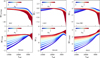 |
Fig. 1 Examples BC dependence on effective temperature in selected HST, LSST, Gaia, Roman, 2MASS, and JWST filters. Filters are ordered by increasing central wavelength. The BCs are color-coded by reddening. |
2.5 Interstellar reddening
Interstellar reddening was also taken into account when determining BCs. We used the ccm89 reddening function of the extinction Python package4. This function uses the reddening law determined by Cardelli et al. (1989). After carrying out several numerical tests, we decided not to redden the BCs but rather to redden the synthetic spectra themselves before determining the BCs. Reddening the spectra was achieved by varying AV between 0.0 and 3.1 in 11 steps with a step size of 0.31 in equation RV = AV/E(B - V), where RV was set to 3.1. This resulted in a 0.1 step size in E(B - V) between E(B - V) = 0 and 1.
2.6 Program package species
From the BOSZ theoretical spectra, our synthetic magnitudes in the Vega magnitude system were determined using the corresponding species Python package routines5 (Stolker et al. 2020). The species software package can use the Spanish Virtual Observatory (SVO) filter profile service6 to retrieve the transmission functions for filters used in instruments of many ground-based observatories and space telescopes. species can automatically choose between the AB and Vega photometric systems. The latter choice can be forced by using the spectrum of Vega. In this case species gives the magnitude values relative to Vega under the assumption that Vega’s brightness is 0.03 mag in all filters by default. While this is mostly true for BVRI filters, it may not be the case for other systems. The zero point depends on the absolute flux used to standardize those systems. This is important to point out, because species does not account for the offsets between systems; therefore, the published magnitudes and BCs may have systematic discrepancies relative to the specific photometric system definitions in the range of a few hundredths of magnitudes in certain filters. At the start of the calculation, it downloads the most recent spectrum of Vega from the CALSPEC database (Bohlin et al. 2014) and calculates the magnitudes for the synthetic spectra using those derived from that. The Vega spectrum used in this paper is alpha_lyr_stis_011.fits, which can be downloaded from the CALSPEC7 database.
3 The scope of the database
The Spanish Virtual Observatory Filter Profile Service (SVO FPS, Rodrigo et al. 2012; Rodrigo & Solano 2020) provides standardized information, including transmission curves and calibration, on more than 7900 astronomical filters. The service is designed to be compliant with the Virtual Observatory Photometry Data Model, and all the information is provided through both a web portal and VO services, enabling other services and applications to access relevant filter properties in a simple way.
We carefully checked the SVO FPS and selected the facil-ity/instrument pairs considered most important for modern astronomical photometry. Our sample contains a total of 752 filters for 78 instruments from 35 ground-based observatories and space telescopes. From the available filter transmission curves, we selected only those with labels indicating use for full-fledged photometric measurements. The facilities, instruments, and the number of filters are listed in Table 1. All filters selected had a minimum wavelength exceeding 50 nm and a maximum wavelength below 32 microns in order to align with the wavelength range covered by the BOSZ spectra.
The parameter space covered by our BC database is almost the same as that of the BOSZ spectral library. The main difference is that in the spectral library the step size of Teff is 100 K below 4000 K, 250 K between 4000 and 12 000 K, and 500 K above 12 000 K, while in our BC database it is 50 K throughout the temperature range. The magnitude and BC values on the denser grid points were determined by a third-order spline interpolation. Due to potentially large flux differences between model spectra, we did not interpolate the spectra themselves to determine the magnitude and BC values for the 50 K step interval. Rather, we performed the interpolation using the calculated magnitude and BC values at the original grid points. No interpolation was performed for the other parameters (log g, [a/M], [C/M], and AV). The parameters of the final grid are listed in Table 2. The Sun BCs and synthetic magnitudes for all filters can be found in Table 3.
List of facilities, instruments, and number of filters used in BC and synthetic magnitude calculations, following the SVO website naming convention.
List of grid parameters used for magnitude and BC calculations.
Synthetic magnitudes and BCs of the Sun following the SVO website naming convention.
3.1 Validation of color-color relationships
To check the accuracy of our synthetic magnitude scale, we compared the observed Gaia-2MASS (Skrutskie et al. 2006) color relationship data with the same colors in our database. The observed and modeled Gaia and 2MASS color indices GBP-GRP and J - Ks are plotted as a function of all relevant physical parameters (Teff, log g, [M/H], [a/M], [C/M], and AV) in Fig. 2. We selected nearly two million common stars from the Gaia DR3 and 2MASS databases, which are plotted with contour lines in Fig. 2. To generate the contours, we used only those stars with magnitudes brighter than 12 in the G filter, errors in G, GBP, and GRP magnitudes less than 0.01, errors in J, H, and Ks magnitudes less than 0.03, and parallax errors less than 10%. The filtering conditions for errors in brightness values are based on the relationships given by Carrasco8 for Gaia DR2. As a result of the cuts, 1 984 111 Gaia-2MASS stars were included in the sample, from which the contour lines were drawn on the colorcolor diagrams. We did not filter for interstellar reddening as the synthetic color indices for all reddening values are plotted in the figure.
Overall, the agreement between the synthetic and the observed colors is very good; however, there are regions in the color space where the synthetic colors do not match the observation. One such region comprises high-temperature stars where either the GBP - GRP color is too red, or the J- Ks color is too blue (or the combination of the two) compared to the color derived from the observations. This discrepancy, nevertheless, is small. The reason behind this discrepancy is currently unknown. The distribution of the synthetic color points forms a “fan” shape much wider than the observation if GBP - GRP > 1.5, where the temperature is lower than 5000-7000 K, while the colors have a narrow distribution if GBP - GRP < 1.5 (the temperature panel of Fig. 2). This occurs because at temperatures higher than 7000 K the rest of the main atmospheric parameters have a much weaker effect on the stellar spectra than at lower temperatures.
The majority of the observed stars are main-sequence stars with solar metallicities (lower branch of the contour lines) and giant stars (upper branch of the contour lines), as seen in the log g panel of Fig. 2. Because the Gaia-2MASS sample is restricted in brightness, the sample does not contain stars with GBP - GRP > 4, which are the very low-temperature main-sequence and giant stars. The data points at the bottom of the fan, shown with blue points in the metallicity panel, represent the metal-poor red dwarfs, which are not in the observed Gaia-2MASS sample.
Some of the discrepancy between synthetic and observed colors comes from the fact that the BOSZ database includes main atmospheric parameters where there are no observed stars to provide a complete grid. One such region is the most metal-rich and α-poor combination, which can be seen as a narrow strip of dark blue points in the α panel of Fig. 2 between J - Ks 1.5 and 2.2. The reddest, extremely metal-rich ([M/H] = 0.75), but non-existing red giants are at GBP - GRP > 4 and J - Ks > 1.5.
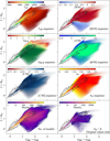 |
Fig. 2 J-Ks vs. GBP-GRP color-color diagram. The contoured area represents stars observed by both Gaia and 2MASS (see Section 3.1 for further details). Each panel is color-coded by a different parameter indicated in the panels themselves. |
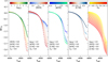 |
Fig. 3 Effects of various parameters on Gaia DR3 BCG. The fixed parameters are listed in the panels. |
3.2 Effect of grid parameters on the bolometric correction
Fig. 3 shows the effect of the astrophysical parameters log g, [M/H], [a/M], [C/M], and AV on Gaia DR3 BCG. In each of the five panels, the values of BCG are plotted against the effective temperature, which varies between 6000 K and 2800 K, and the effects of the other four parameters are indicated by color codes. The fixed parameters are shown in the lower left of the panels in Fig. 3. For log g, the abundance values were set to the solar value of 0.0 dex, while for the abundance panels the log g value was set to 2.0 dex, i.e., the figure only shows the case of giant stars. In each case, the BC starts from around 0.0 at the higher-temperature end of the range, then decreases sharply around 4500 K and becomes increasingly negative. It is clear that below this temperature, all four atmospheric parameters (log g, [M/H], [a/M], and [C/M]) have an effect on the BC, which can even exceed 1.5 magnitudes below 3000 K. In most cases log g and [M/H] have the strongest effect on the BC, but as the temperature decreases [a/M] and [C/M] become important factors for cool stars.
To date, the effect of carbon on the Gaia DR3 G BC has not been studied. By using the BOSZ database, it became possible to examine how [C/M] values affect the BC. This can be seen in the fourth panel of Fig. 3. While low [C/M] values have little effect on the BC, values of [C/M] higher than 0-0.25 dex can affect the BC almost as much as or more than the [a/M] dimension. Below 4500 K carbon has a significant effect on the structure of stellar atmospheres, which must be accounted for during model atmosphere calculations, as implemented in the BOSZ grid. Thus, for carbon-enriched stars it is important to address their carbon content when calculating their luminosity and radius.
Interstellar reddening has a significant effect on BCs and should not be ignored, as emphasized for example by Chen et al. (2019). As mentioned above, the spectra themselves were reddened instead of BCs. The effect of reddening between AV = 0.0 and 3.1 on the Gaia DR3 G BC can be seen in the last panel of Fig. 3. Higher reddening significantly decreases the BC, although the correlation between the two parameters is not linear.
4 Comparing Gaia DR3 G bolometric corrections with literature
Here, we discuss the differences in the official Gaia DR3 G BCs (Creevey et al. 2023) and those presented in this paper. The Gaia DR3 BC software tool also used a MARCS model grid from Gustafsson et al. (2008) up to 8000 K (extending to other spectrum libraries above that value; see Table 2 in Creevey et al. (2023), with a slightly wider range of Teff than our new BOSZ models, from 2500 to 20 000 K. The values of log g differ only at the upper limit, ranging up to 5.0 for Gaia DR3. Its metallicity range of −5.0 to +1.5 is wider than the range of the new BOSZ models; however, the BOSZ models cover a wider range of [a/M]values. In Creevey et al. (2023), the a-element enhancement range spans from 0.0 to +0.4. The most significant difference between the two model grids is that the new BOSZ models account for carbon contribution, whereas the Gaia DR3 G BCs do not.
The difference between the Gaia DR3 G BCs and those of Creevey et al. (2023) for the same parameters is shown in Fig. 4 as a function of Teff. To explore the effects of the updates made on the BOSZ grid compared to the synthetic spectra of Gustafsson et al. (2008), the constant offset of 0.2 applied to Gaia DR39 was removed. Additionally, their adopted value for the Sun’s BC is BCG,⊙ = +0.08 mag, while ours directly comes from the model and is equal to 0.0464 mag (see Table 3). By correcting for this offset as well, the difference seen in Fig. 4 is only due to differences in the synthetic spectral grid used in the calculations.
A large systematic offset that slightly correlates with temperature can be seen for the hot stars above 8000 K. This is probably the result of differing model atmospheres: Gaia DR3 used the line-by-line opacity stellar model atmospheres from Shulyak et al. (2004), while the BOSZ database used ATLAS9 models from Mészáros et al. (2012). The right panel of Fig. 4 shows the Teff < 8000 K range in more detail. Although the agreement between the two BCs is better than 0.02 magnitude in the 8000-4000 K range, significant temperaturedependent systematic offsets can be seen again below 4000 K. This is the temperature regime where molecules dominate the spectrum and the BOSZ grid implements newer, more up-to-date molecular line lists - mostly from the EXOMOL project (Barton et al. 2017a,b) - compared to those available to Gustafsson et al. (2008).
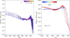 |
Fig. 4 Difference between the BCG from this paper and from Gaia DR3 as a function of Teff. Left: all common Teff, log g, and [M/H] combinations. Right: log g set to 4.5 to reveal the metallicity-dependent differences on the main sequence. [α/M] = [C/M] = 0.0 in both cases. |
5 APOGEE luminosities
5.1 Our APOGEE sample
To determine new luminosity values for the APOGEE survey (Majewski et al. 2017), we first compiled a list of stars detected by both Gaia DR3 and APOGEE DR17 (Abdurro’uf et al. 2022), then filtered this list according to several criteria. Only APOGEE targets without the BAD flag are included in the list. To filter out binaries and pulsating variables, we considered only targets for which the APOGEE parameter vscatter (the scatter of radial velocities derived from spectra taken at different times) is less than 1 km s−1. In addition, we also required that the error in individual radial velocities not exceed 1 km s−1. Finally, we removed targets with a parallax error exceeding 10%. This process resulted in a sample of 192 049 stars.
After filtering as described above, we applied additional cuts, because a and carbon abundances are unreliable in certain parameter ranges (for more details, see Jönsson et al. 2020; Mészáros et al. 2025). For effective temperatures below 4500 K, only stars with a log g value less than 3.0 were considered, because carbon abundances of red dwarfs are not reliable. As explored by Mészáros et al. (2025), stars with effective temperatures lower than 4250 K and [C/M] higher than 0.1 also have unreliable abundances; thus, it is necessary to exclude cool, carbon-rich stars from the sample. After cutting, the sample contained 177 728 targets that met the requirements. We note that this sample still contained some metal- and carbon-rich stars above 4250 K, with [C/M] values reaching 0.25 dex.
Fig. 5 shows the new luminosities as functions of the effective temperature for our APOGEE sample calculated using Equations (13) and (14). Here, BCG values were derived with radial basis function interpolation using the calibrated astrophysical parameters Teff, log g, [M/H], [a/M], raw (uncalibrated) [C/M] and E(B - V) published in APOGEE DR17. Because we excluded the red dwarfs from the sample, a straight vertical boundary is observed at 4500 K, below which only a handful of stars are seen due to probable incorrect luminosity calculations.
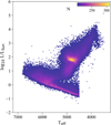 |
Fig. 5 HRD of our selected APOGEE targets using the new Gaia DR3 BCG values presented in this paper. |
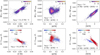 |
Fig. 6 Error in BC (top panels) and luminosity (bottom panels) caused by fixing carbon, alpha, and metallicity at zero for stars with log g < 3.6. The values BCG and L were calculated with all three parameters taken into account, and the “mod.” (modified) values show the effect when one or several of the parameters - [M/H], [α/M], and [C/M] - are fixed to zero. The value N denotes the number of stars for BC. |
5.2 The effect of carbon on bolometric correction and luminosity
Fig. 6 shows the effect on BC (top) and luminosity (bottom) when certain parameters are not account for during BC determination. Only RGB (red-giant branch) stars with log g < 3.6 are selected here to remove erroneous measurements of the abundances in the main sequence. On the vertical axis, the values BCG and L were calculated with all three parameters taken into account. Moreover, the “mod.” (modified) values show the effect when one or several of the parameters - [M/H], [a/M], and [C/M] - values are fixed to zero. As indicated in the figure, in the first column [C/M] was set to 0.0, but [M/H], and [a/M] were taken from APOGEE; in the second column [C/M] = [a/M] = 0.0, but metallicity was allowed to vary; and in the last column, all three parameters were set to zero, meaning only Teff , log g, and the reddening were taken into account.
The effect on BCs is given as a magnitude difference, whereas the effect on luminosities is expressed in relative terms. The histograms are colored by the number of stars. It can be clearly seen that ignoring all three parameters causes errors of up to 0.04 magnitude and up to 1% in BC and luminosity across the full temperature range. We note a clear correlation between the BC difference and the [M/H] value of the star. Of course, the errors decrease once metallicity and a elements are considered. However, if carbon is not used in the BC calculation, at 45005000 K - where most of the stars reside - around 0.005 mag and 0.2% error remains in BC and luminosity, respectively. A correlation can be seen between BC differences and [C/M] values when [a/M] and [M/H] are considered but [C/M] is not (top left panel of Fig. 6). These trends are also mirrored in luminosity with opposite signs. This is an expected behavior, because as shown in Section 3.2 the value of BCG increases with increasing [C/M]. Thus, ignoring - as opposed to including - carbon produces lower BCG values and decreases luminosity.
6 Overview
In this paper, we presented a new, extensive database of synthetic stellar magnitudes and BCs based on the latest BOSZ spectral library. Our goal is to improve estimates of stellar luminosities by delivering accurate BCs across hundreds of photometric filters. In the Gothard Observatory Synthetic Stellar Photometry Database, synthetic magnitudes were computed in the Vega system using the Python package species, and BCs were derived from fundamental flux-magnitude relationships, by applying interstellar reddening directly to the spectra via Cardelli’s extinction law. Covering 752 filters from 78 instruments (ground- and space-based), the database spans effective temperatures from 2800 to 16 000 K, log g from −0.5 to 5.5, metallicity from −2.5 to 0.75, [a/M] from −0.25 to 0.5, [C/M] from −0.75 to 0.5, and reddening up to AV = 3.1 mag. Using high-resolution (R = 50 000) synthetic spectra allowed us to precisely track the effect of abundances on the BCs and luminosities of stars.
Validation against nearly two million Gaia-2MASS stars shows strong agreement in color-color space, with minor discrepancies at extreme temperatures. Compared to existing Gaia DR3 BCs, our corrections differ by up to 0.2 mag for hot stars and up to 0.12 mag below 4000 K probably due to the improved treatment of molecular opacities in the BOSZ database. By applying the new BCs to 192000 APOGEE stars, we calculated refined luminosities and also demonstrated that neglecting carbon or α enhancements can introduce up to 1% errors in luminosity. Overall, the new Gothard Observatory Synthetic Stellar Photometry Database may enable more accurate fundamental parameter determinations for large stellar samples using a vast amount of past, present, and upcoming surveys, such as Gaia, LSST, and the Roman Space Telescope.
Data availability
The full table 3 is available at the CDS via https://cdsarc.cds.unistra.fr/viz-bin/cat/J/A+A/706/A318.
The database can be downloaded in part or in its entirety from https://gosspd.gothard.hu/data.
Acknowledgements
This project has been supported by the LP2021-9 Lendület grant of the Hungarian Academy of Sciences. On behalf of the “Calculating the Synthetic Stellar Spectrum Database of the James Webb Space Telescope” project, we are grateful for the possibility to use HUN-REN Cloud (see Héder et al. 2022; https://science-cloud.hu) which helped us achieve the results published in this paper. This project has received funding from the HUN-REN Hungarian Research Network, and support from the National Research, Development and Innovation Office (NKFIH, Hungary) through grants SNN-147362 and ADVANCED-153410, as well as from ESA PRODEX Experiment through Agreements No. 4000137122 and No. 4000149203. Funding for the Sloan Digital Sky Survey IV has been provided by the Alfred P. Sloan Foundation, the U.S. Department of Energy Office of Science, and the Participating Institutions. SDSS-IV acknowledges support and resources from the Center for High Performance Computing at the University of Utah. The SDSS website is www.sdss.org. SDSS-IV is managed by the Astrophysical Research Consortium for the Participating Institutions of the SDSS Collaboration including the Brazilian Participation Group, the Carnegie Institution for Science, Carnegie Mellon University, Center for Astrophysics I Harvard & Smithsonian, the Chilean Participation Group, the French Participation Group, Instituto de Astrofísica de Canarias, The Johns Hopkins University, Kavli Institute for the Physics and Mathematics of the Universe (IPMU) / University of Tokyo, the Korean Participation Group, Lawrence Berkeley National Laboratory, Leibniz Institut für Astrophysik Potsdam (AIP), Max-Planck-Institut für Astronomie (MPIA Heidelberg), Max-Planck-Institut für Astrophysik (MPA Garching), Max-Planck-Institut für Extraterrestrische Physik (MPE), National Astronomical Observatories of China, New Mexico State University, New York University, University of Notre Dame, Observatário Nacional / MCTI, The Ohio State University, Pennsylvania State University, Shanghai Astronomical Observatory, United Kingdom Participation Group, Universidad Nacional Autónoma de México, University of Arizona, University of Colorado Boulder, University of Oxford, University of Portsmouth, University of Utah, University of Virginia, University of Washington, University of Wisconsin, Vanderbilt University, and Yale University. This research has made use of the SVO Filter Profile Service “Carlos Rodrigo”, funded by MCIN/AEI/10.13039/501100011033/ through grant PID2020-112949GB-I00.
References
- Abdurro’uf, Accetta, K., Aerts, C., et al. 2022, ApJS, 259, 35 [NASA ADS] [CrossRef] [Google Scholar]
- Barton, E. J., Hill, C., Czurylo, M., et al. 2017a, J. Quant. Spec. Radiat. Transf., 203, 490 [CrossRef] [Google Scholar]
- Barton, E. J., Hill, C., Yurchenko, S. N., et al. 2017b, J. Quant. Spec. Radiat. Transf., 187, 453 [CrossRef] [Google Scholar]
- Bohlin, R. C., Gordon, K. D., & Tremblay, P. E. 2014, PASP, 126, 711 [NASA ADS] [Google Scholar]
- Bohlin, R. C., Mészáros, S., Fleming, S. W., et al. 2017, AJ, 153, 234 [Google Scholar]
- Buser, R. 1986, Highlights Astron., 7, 799 [Google Scholar]
- Cardelli, J. A., Clayton, G. C., & Mathis, J. S. 1989, ApJ, 345, 245 [Google Scholar]
- Casagrande, L., & VandenBerg, D. A. 2014, MNRAS, 444, 392 [Google Scholar]
- Casagrande, L., & VandenBerg, D. A. 2018a, MNRAS, 479, L102 [NASA ADS] [CrossRef] [Google Scholar]
- Casagrande, L., & VandenBerg, D. A. 2018b, MNRAS, 475, 5023 [Google Scholar]
- Chambers, K. C., Magnier, E. A., Metcalfe, N., et al. 2019, The Pan-STARRS1 Surveys [Google Scholar]
- Chen, Y., Girardi, L., Fu, X., et al. 2019, A&A, 632, A105 [EDP Sciences] [Google Scholar]
- Cohen, M., Witteborn, F. C., Carbon, D. F., et al. 1996, AJ, 112, 2274 [Google Scholar]
- Cousins, A. W. J. 1976, MmRAS, 81, 25 [Google Scholar]
- Creevey, O. L., Sordo, R., Pailler, F., et al. 2023, A&A, 674, A26 [NASA ADS] [CrossRef] [EDP Sciences] [Google Scholar]
- Fitzpatrick, E. L. 1999, PASP, 111, 63 [Google Scholar]
- Gaia Collaboration (Prusti, T., et al.) 2016, A&A, 595, A1 [NASA ADS] [CrossRef] [EDP Sciences] [Google Scholar]
- Gaia Collaboration (Brown, A. G. A., et al.) 2018, A&A, 616, A1 [NASA ADS] [CrossRef] [EDP Sciences] [Google Scholar]
- Gaia Collaboration (Vallenari, A., et al.) 2023, A&A, 674, A1 [NASA ADS] [CrossRef] [EDP Sciences] [Google Scholar]
- Grevesse, N., Asplund, M., & Sauval, A. J. 2007, Space Sci. Rev., 130, 105 [Google Scholar]
- Gustafsson, B., Edvardsson, B., Eriksson, K., et al. 2008, A&A, 486, 951 [NASA ADS] [CrossRef] [EDP Sciences] [Google Scholar]
- Hubeny, I., Prieto, C. A., Osorio, Y., & Lanz, T. 2021, TLUSTY and SYNSPEC Users’s Guide IV, Upgraded Versions 208 and 54 [Google Scholar]
- Héder, M., Rigó, E., Medgyesi, D., et al. 2022, InfTars - Információs Tár-sadalom, 2, 10 [Google Scholar]
- Jönsson, H., Holtzman, J. A., Allende Prieto, C., et al. 2020, AJ, 160, 120 [Google Scholar]
- Keller, S. C., Schmidt, B. P., Bessell, M. S., et al. 2007, PASA, 24, 1 [NASA ADS] [CrossRef] [Google Scholar]
- Kurucz, R. L. 1979, ApJS, 40, 1 [NASA ADS] [CrossRef] [Google Scholar]
- Mamajek, E. E., Torres, G., Prsa, A., et al. 2015, arXiv e-prints [arXiv:1510.06262] [Google Scholar]
- Majewski, S. R., Schiavon, R. P., Frinchaboy, P. M., et al. 2017, AJ, 154, 94 [NASA ADS] [CrossRef] [Google Scholar]
- Mészáros, S., Allende Prieto, C., Edvardsson, B., et al. 2012, AJ, 144, 120 [Google Scholar]
- Mészáros, S., Bohlin, R., Allende Prieto, C., et al. 2024, A&A, 688, A197 [NASA ADS] [CrossRef] [EDP Sciences] [Google Scholar]
- Mészáros, S., Jofré, P., Johnson, J. A., et al. 2025, AJ, 170, 96 [Google Scholar]
- Oke, J. B. 1974, ApJS, 27, 21 [Google Scholar]
- Rodrigo, C., & Solano, E. 2020, in XIV.0 Scientific Meeting (virtual) of the Spanish Astronomical Society, 182 [Google Scholar]
- Rodrigo, C., Solano, E., & Bayo, A. 2012, SVO Filter Profile Service Version 1.0, IVOA Working Draft 15 October 2012 [Google Scholar]
- Shulyak, D., Tsymbal, V., Ryabchikova, T., Stütz, C., & Weiss, W. W. 2004, A&A, 428, 993 [NASA ADS] [CrossRef] [EDP Sciences] [Google Scholar]
- Shulyak, D., Valyavin, G., Kochukhov, O., Khan, S., & Tsymbal, V. 2005, Mem. Soc. Astron. Ital. Suppl., 7, 99 [Google Scholar]
- Skrutskie, M. F., Cutri, R. M., Stiening, R., et al. 2006, AJ, 131, 1163 [NASA ADS] [CrossRef] [Google Scholar]
- Stolker, T., Quanz, S. P., Todorov, K. O., et al. 2020, A&A, 635, A182 [EDP Sciences] [Google Scholar]
- Straizys, V. 1996, Baltic Astron., 5, 459 [Google Scholar]
- STScI Development Team 2018, synphot: Synthetic photometry using Astropy, Astrophysics Source Code Library [record ascl:1811.001] [Google Scholar]
- Tennyson, J., & Yurchenko, S. N. 2012, MNRAS, 425, 21 [Google Scholar]
- Tennyson, J., Yurchenko, S. N., Al-Refaie, A. F., et al. 2016, J. Mol. Spectrosc., 327, 73 [Google Scholar]
An updated version of their BC database for Gaia DR3 is available on L. Casagrande’s GitHub page. See https://github.com/casaluca/bolometric-corrections
All Tables
List of facilities, instruments, and number of filters used in BC and synthetic magnitude calculations, following the SVO website naming convention.
Synthetic magnitudes and BCs of the Sun following the SVO website naming convention.
All Figures
|
Fig. 1 Examples BC dependence on effective temperature in selected HST, LSST, Gaia, Roman, 2MASS, and JWST filters. Filters are ordered by increasing central wavelength. The BCs are color-coded by reddening. |
| In the text | |
|
Fig. 2 J-Ks vs. GBP-GRP color-color diagram. The contoured area represents stars observed by both Gaia and 2MASS (see Section 3.1 for further details). Each panel is color-coded by a different parameter indicated in the panels themselves. |
| In the text | |
|
Fig. 3 Effects of various parameters on Gaia DR3 BCG. The fixed parameters are listed in the panels. |
| In the text | |
|
Fig. 4 Difference between the BCG from this paper and from Gaia DR3 as a function of Teff. Left: all common Teff, log g, and [M/H] combinations. Right: log g set to 4.5 to reveal the metallicity-dependent differences on the main sequence. [α/M] = [C/M] = 0.0 in both cases. |
| In the text | |
|
Fig. 5 HRD of our selected APOGEE targets using the new Gaia DR3 BCG values presented in this paper. |
| In the text | |
|
Fig. 6 Error in BC (top panels) and luminosity (bottom panels) caused by fixing carbon, alpha, and metallicity at zero for stars with log g < 3.6. The values BCG and L were calculated with all three parameters taken into account, and the “mod.” (modified) values show the effect when one or several of the parameters - [M/H], [α/M], and [C/M] - are fixed to zero. The value N denotes the number of stars for BC. |
| In the text | |
Current usage metrics show cumulative count of Article Views (full-text article views including HTML views, PDF and ePub downloads, according to the available data) and Abstracts Views on Vision4Press platform.
Data correspond to usage on the plateform after 2015. The current usage metrics is available 48-96 hours after online publication and is updated daily on week days.
Initial download of the metrics may take a while.