| Issue |
A&A
Volume 706, February 2026
|
|
|---|---|---|
| Article Number | A321 | |
| Number of page(s) | 10 | |
| Section | Astrophysical processes | |
| DOI | https://doi.org/10.1051/0004-6361/202557862 | |
| Published online | 17 February 2026 | |
Double-hump spectrum, pulse profile dip, and pulsed fraction spectra from the low-accretion regime in the X-ray pulsar MAXI J0655-013
1
INAF-Osservatorio Astronomico di Roma Via Frascati 33 I-00078 Monte Porzio Catone (RM), Italy
2
Department of Astronomy and Astrophysics, University of California San Diego CA 92093, USA
3
INAF – IASF Palermo Via Ugo La Malfa 153 90146 Palermo, Italy
4
Department of Astronomy and Astrophysics, University of California San Diego La Jolla CA 92075, USA
5
Institut für Astronomie und Astrophysik, Universität Tübingen Sand 1 D-72076 Tübingen, Germany
6
Institute of Space Sciences (ICE, CSIC), Campus UAB Carrer de Can Magrans s/n E-08193 Barcelona, Spain
7
Institut d’Estudis Espacials de Catalunya (IEEC) 08860 Castelldefels Barcelona, Spain
8
European Space Agency (ESA), European Space Astronomy Centre (ESAC) Camino Bajo del Castillo s/n 28692 Villanueva de la Cañada Madrid, Spain
9
Università Tor Vergata, Dipartimento di Fisica Via della Ricerca Scientifica 1 I-00133 Rome, Italy
10
Department of Physics and Astronomy, Howard University Washington DC 20059, USA
11
CRESST and NASA Goddard Space Flight Center, Astrophysics Science Division 8800 Greenbelt Road Greenbelt MD, USA
12
Dipartimento di Fisica e Chimica E. Segrè, Università degli Studi di Palermo Via Archirafi 36 90123 Palermo, Italy
13
Physics Department, United States Naval Academy Annapolis MD 21402, USA
14
Department of Physics and Astronomy, Embry-Riddle Aeronautical University 3700 Willow Creek Road Prescott AZ 86301, USA
15
Dr. Karl-Remeis-Observatory and Erlangen Centre for Astroparticle Physics, Friedrich-Alexander-Universität Erlangen-Nürnberg Sternwartstr. 7 96049 Bamberg, Germany
★ Corresponding author: This email address is being protected from spambots. You need JavaScript enabled to view it.
Received:
27
October
2025
Accepted:
22
December
2025
Abstract
Context. Accreting X-ray pulsars (XRPs) undergo different physical regimes depending on different mass accretion rates, with related changes in the emitted X-ray spectral properties. Recent observations have shown a dramatic change in the emission properties of this class of sources observed at low luminosity.
Aims. We explore the timing and spectral properties of the XRP MAXI J0655-013 observed in the low-luminosity regime (about 5 × 1033 erg s−1) to witness the corresponding spectral shape and pulse profiles.
Methods. We employed recent XMM-Newton and NuSTAR pointed observations of the MAXI J0655-013 X-ray activity during the low-luminosity stage. We explored several spectral models to fit the data and test theoretical expectations of the dramatic transition of the spectral shape compared to the higher luminosity regime. We studied the pulsating nature of the source and found a precise timing solution. We explored the energy-resolved pulse profiles and the derived energy dependence of different pulsed fraction estimators (PFminmax and PFrms). We also obtained NuSTAR pulsed fraction spectra (PFS) at different luminosity regimes.
Results. The MAXI J0655-013 spectrum is well fit by a double Comptonization model, in agreement with recent observational results and theoretical expectations that explain the observed spectrum as being composed of two distinct bumps, each dominated by different polarization modes. We measured a spin period of 1081.86 ± 0.02 s, consistent with the source spinning up compared to previous observations, yielding an upper limit for the magnetic field strength of B ≲ 9 × 10¹³ G. The pulse profiles show a single broad peak interrupted by a sharp dip that coincides with an increase in the hardness ratio, and thus likely due to absorption. For the low-luminosity observation, the PFminmax increases with energy up to ∼100% in the 10–30 keV band, while the PFrms remains steady at ∼60%. The PFS obtained at high luminosity shows evidence of an iron Kα emission line but no indications of a cyclotron line.
Key words: accretion / accretion disks / polarization
© The Authors 2026
 Open Access article, published by EDP Sciences, under the terms of the Creative Commons Attribution License (https://creativecommons.org/licenses/by/4.0), which permits unrestricted use, distribution, and reproduction in any medium, provided the original work is properly cited.
This article is published in open access under the Subscribe to Open model. This email address is being protected from spambots. You need JavaScript enabled to view it. to support open access publication.
1. Introduction
MAXI J0655-013 (J0655 hereafter) is an accreting X-ray pulsar (XRP) recently discovered (Serino et al. 2022; Kennea et al. 2022; Nakajima et al. 2022) during an outburst episode that allowed its spectral and timing broadband study with NuSTAR (Pike et al. 2023, and references therein). Besides that one outburst episode, the source has not shown any evident X-ray activity. The optical companion is a B1-3e III-V star, implying that the system is a Be/X-ray binary (BeXRB, Reig et al. 2022). The pulsar is a slowly rotating neutron star (NS) with a spin period of about 1100 s (Shidatsu et al. 2022; Pike et al. 2023). The broadband NuSTAR continuum spectrum of the source was fit with the typical model employed for this class of sources, i.e., a cutoff power-law model (Pike et al. 2023). The magnetic field strength for this source has been estimated to be in the range 0.5 − 50 × 1013 G (Pike et al. 2023). The wide range of magnetic field values derives from the different methods employed to infer it, including a tentative cyclotron line at 44 keV. The line was, however, interpreted with caution by the authors for several reasons, for example, the width of the line is too narrow to be consistent with other similar sources and accretion conditions. A distance of  kpc was measured by Gaia Data Release 3 (DR3) (Gaia Collaboration 2023). Given this distance value, Pike et al. (2023) measured the source X-ray luminosity at the early and late stages of the 2022 outburst as 5.6 × 1036 erg s−1 and 4 × 1034 erg s−1, respectively.
The spectral energy distribution of accreting XRPs observed during bright (∼1036 erg s−1) outburst episodes is typically fit using a phenomenological cutoff power-law model (Nagase 1989; Caballero & Wilms 2012; Mushtukov & Tsygankov 2022). While this approach is a useful first approximation, it does not provide insights into the ongoing accretion physics. In fact, the computation of physical parameters needs to account for magnetic, thermal, and bulk Compton scattering, cyclotron emission and absorption, blackbody radiation from multiple regions, and magnetic bremsstrahlung (Becker & Wolff 2022, and references therein). However, recent studies of XRPs observed at low-mass accretion rates (thus low luminosity values, i.e., ∼1033 − 1034 erg s−1) have highlighted that the spectrum observed in this regime shows a substantially different shape. In fact, the spectral distribution observed at low luminosity often shows two main distinct components, indicated as a double-hump spectrum (Tsygankov et al. 2019a,b; Lutovinov et al. 2021). This is interpreted as the result of different mechanisms occurring at spatially separate sites, as detailed in the following. The upper layers of the atmosphere are overheated (compared to the lower layers) by residual accretion. At the same time, seed blackbody photons are produced by magnetic free-free emission in the lower part of the atmosphere near the NS surface. While collisions cause the braking of accretion in the atmosphere, resulting in the excitation of electrons to upper Landau levels, the subsequent radiative de-excitation of electrons produces cyclotron photons. Cyclotron and free-free photons reprocessed by resonant Comptonization in an atmosphere with a strong temperature gradient are responsible for the high-energy bump peaking around 30 keV, while the absorbed part is then released mostly as extra-ordinary polarized photons from the bottom part of the atmosphere, thus forming the low-energy bump peaking around 5 keV (Mushtukov et al. 2021; Sokolova-Lapa et al. 2021).
For this work, we have taken advantage of pointed X-ray observations of the accreting XRP MAXI J0655 in order to study its low-luminosity spectral and timing properties. Due to its residual accretion, its vicinity, an estimation of its magnetic field, and a relatively unobscured line of sight, MAXI J0655 is an ideal target to unveil the processes responsible for the characteristic spectral shape and the accompanying timing features in the low-luminosity regime.
2. Observations and data reduction
A light curve of MAXI J0655 as observed by our pointed XMM-Newton and NuSTAR observations is shown in Fig. 1. Observations are separated by a 1-week gap. In the following, we illustrate the data reduction procedure for each dataset.
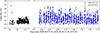 |
Fig. 1. XMM-Newton (0.5–10 keV) and NuSTAR (4–79 keV) both at 100 s binning light curves of MAXI J0655. Count rates were rescaled according to model predictions and effective area accounting for the observed spectral energy distribution. |
2.1. XMM-Newton observations
XMM-Newton observed MAXI J0655 on September 26, 2024 (MJD 60579, see Table 1). ObsID 0935630101 was carried out in Full Frame mode. XMM-Newton data were reduced using the XMM-Newton Science Analysis System (SAS) v21.0.0 and the latest available calibration files (XMM-CCF-REL-403). We followed the standard procedure described in SAS Data Analysis Threads for data reduction1. Due to high solar activity, the effective exposure was reduced from the nominal 66 ks to about 40 ks for EPIC-MOS and 25 ks for EPIC-pn.
Log of MAXI J0655 observations used in this work.
After standard cleaning of the raw data, events were extracted from a circular region centered on the source with a radius of 24″, while background events were extracted from a 75″-radius circular source-free region on the same chip. Spectral response files were generated using the rmfgen and arfgen tasks. We also applied a correction to the effective area suited for simultaneous spectral fitting of EPIC and NuSTAR spectra available through the applyabsfluxcorr=yes option. We verified through the epatplot tool that pile-up did not affect our spectra.
Finally, we also extracted EPIC-pn and EPIC-MOS spectra for GTIs where the flaring particle background was high. We then compared these spectra with those obtained from events outside the flaring activity period. The spectra obtained from the flaring part of the data were fully consistent with those obtained by filtering out the high-flaring period. Therefore, we merged the resulting spectra and responses using the epicspeccombine tool, increasing the exposures by about 6 ks and 16 ks for EPIC-MOS and EPIC-pn, respectively. We also verified that both in the case when individual spectra are used for the NuSTAR joint fit, and in the case when the XMM-Newton merged spectra are used, the same cross-calibration constant value is obtained (see Sect. 3).
2.2. NuSTAR
NuSTAR observed MAXI J0655 on October 10, 2024 (MJD 60593, ObsID 31001020002). NuSTAR data were reduced with NUSTARDAS v2.1.2 using the CALDB 20240729 (Madsen et al. 2021). The cleaned events were obtained following the standard NuSTAR guidelines. Source spectra were extracted through the NUPRODUCTS routine. The source extraction region was a circular region of 50″ centered on the source, while background events were extracted from a 90″ circular region of a source-free area on the same detector. Due to increased Solar activity during observation, an additional background filtering based on the South Atlantic Anomaly (SAA) tentacles and space weather conditions was applied (saacalc = 2 saamode=OPTIMIZED tentacle=yes). However, we verified that such strict filtering does not yield an improvement in the flaring background, at the expense of a considerable part of the exposure, compared to the employment of the OPTIMIZED option for SAA filtering alone. Therefore, we opted for the latter filtering. The resulting total filtered exposure time was approximately 83 ks.
2.3. Swift/XRT
Upon further research of archival data, the source was found to be already known from the Improved and Expanded version of the Neil Gehrels Swift X-ray Telescope Point Source Catalog as 2SXPS J065512.4-012855 (Evans et al. 2020), where it was serendipitously cataloged as an X-ray source. Swift/XRT observed this source on May 23, 2018 (MJD 58261, ObsID 03101816001). The source was observed in photon counting mode for a total of about 1 ks (see Table 1). We extracted XRT data products using the online platform (Evans et al. 2009) provided by the UK Swift Data Centre2.
3. Spectral analysis
We analyzed spectral data using XSPEC v12.13.1 (Arnaud 1996) as part of HEASOFT v6.33.1. XMM-Newton spectral data were rebinned using the specgroup routine with the standard value of 25 counts per bin and an oversampling factor of the intrinsic energy resolution of up to 3, while NuSTAR spectra were rebinned with the ftgrouppha HEASARC tool with the Kaastra & Bleeker (2016) optimal binning and the additional requirement of a minimum number of 25 counts per bin. We employ χ2 as the test statistic, and Cash statistic (Cash 1979) with Poissonian background, that is, W-stat, as the fit statistic. The photoelectric absorption component (or column density NH) was set according to Wilms et al. (2000, tbabs in XSPEC), and we assumed model-relative (wilm) elemental abundances.
Given that the source was observed in the low-luminosity regime, we expect the spectrum to exhibit a double-hump shape. Thus, we modeled the data with two separate Comptonization components, CompTT (Titarchuk 1994) in the XSPEC terminology, setting a cross-normalization constant to account for calibration uncertainties between the instruments. The resulting best-fit is shown in Fig. 2. For this model, the test statistic divided by the degrees of freedom (d.o.f.) is χ2/d.o.f. = 491/478. For comparison, we also tested different models in which only one continuum component is employed, modified by a discrete feature with a Gaussian absorption or emission profile (respectively, gabs or Gauss in the XSPEC terminology). Similar models have been tested in other XRPs, e.g., the CompTT*gabs model for the case of X-Persei, (Doroshenko et al. 2012), the CompTT+Gauss model, and the Cutoffpl*gabs model. The resulting χ2/d.o.f. are 495/478, 692/478, and 513/478, respectively. However, despite being statistically comparable to the CompTT + CompTT best-fit model, the Cutoffpl*gabs model returns unphysical best-fit parameters, such as a depth of the absorption line of  keV at 1σ c.l., and therefore it is not considered further. Our spectral results are reported in Table 2 for the two aforementioned models that are supported by the test statistics and the physical values of their best-fit parameters. On the other hand, because our data do not allow us to constrain the high-energy curvature component in the double CompTT model, we also tested a model consisting of an absorbed blackbody with a power-law tail. This model returns a larger test statistic, χ2/d.o.f. = 521/470. Its best-fit blackbody temperature and radius are
  keV and
  m, respectively, while the photon index is 1.60 ± 0.04. Finally, following Salganik et al. (2025), we also tested a double CompTT model in which the optical depth of the high-energy CompTT component is frozen to τp = 100. The resulting test statistic is comparable to that obtained when the parameter value is let free. Also, the resulting temperature of the hot CompTT component is better constrained,
  keV. It is hard, however, to reconcile such a high optical depth with a physical plasma at a temperature this high and in the low accretion rate regime. We therefore will not consider this fit as a viable model.
 |
Fig. 2. Unfolded spectra from XMM-Newton pn, MOS 1, and 2 (black, red, and green, respectively) and NuSTAR FPMA and FPMB (blue and cyan, respectively) from the MAXI J0655 observations in the low-luminosity regime analyzed in this work. Dashed lines represent the two Comptonization components for each instrument. Bottom panel: residuals to the best-fit double-CompTT model. |
Best-fit parameters of MAXI J0655 data from XMM-Newton+NuSTAR observations for two different spectral models.
The value of the cross-calibration constant between XMM-Newton and NuSTAR detectors differs by about 40%. This is higher than the ∼20% difference expected from known calibration issues3, implying that the XMM-Newton recovered flux is systematically lower than that measured by NuSTAR by about 20%. Despite the correction for the calibration issues being applied (see Sect. 2.1), we note that this correction only extends down to 3 keV for the XMM-Newton response file (see also Kang & Wang 2024). We conclude that the difference observed in the cross-correlation constants is likely due to calibration issues and partially due to intrinsic source variability, to a factor that is at least equal to the remaining 20% difference.
As a result of the different cross-calibration constant values, the source unabsorbed luminosity (in the 0.1–100 keV range) is 5.8(1)×1033 erg s−1 as observed by XMM-Newton-pn, while it is 1.4(1)×1034 erg s−1 as observed by NuSTAR (for an assumed distance of 3.6 kpc). For comparison, we also report the results of the Swift/XRT observation of MAXI J0655 in 2018. The faint spectrum can be fit either with a power-law model or a blackbody model. Given how faint the source is and the short exposure, the best-fit parameters are not firmly constrained. However, for both models, we obtain a value of the unabsorbed flux (in the 0.3–10 keV energy band) of  erg cm−2 s−1, corresponding to a luminosity of ∼2 × 1033 erg s−1. We notice that this flux value is in broad agreement with that obtained by XMM-Newton (see Table 2), thus supporting the hypothesis that the source actually underwent a moderate accretion-rate change between the XMM-Newton and NuSTAR observations, separated by about a week.
4. Timing analysis
Given the long spin period of MAXI J0655 and the length of NuSTAR exposure, we first used NuSTAR products for the timing analysis. We followed a procedure similar to the one presented in Pike et al. (2023) for determining the pulse period. First, we barycentered the events using the barycorr tool and NuSTAR clockfile nuCclock20100101v209. Next, we used Stingray (Huppenkothen et al. 2019) to perform a coarse Zn2 search (Buccheri et al. 1983) with n = 4 in the mHz range. We found one significant peak near the previously measured pulse period. Using the results of this coarse search, we next performed a fine search on the highest peak to determine the pulse period more precisely. We fit a cubic spline to the Z42(ν) distribution resulting from the fine search and determined the pulse period corresponding to the peak of this distribution, that is P = 1082.0 s (ν = 0.9242 mHz).
Finally, we used both XMM-Newton and NuSTAR datasets together, along with a phase-fitting technique (Deeter et al. 1981) to infer the best possible value of the period, which resulted in P = 1081.86 ± 0.02 s (ν = 0.92433(1) mHz; uncertainties at 1σ for one parameter of interest). For this, we used a sinusoidal template profile in the overlapping energy band between the instruments and used the phase corresponding to the midway point between the maximum and the minimum values of the sinusoidal profile. Pike et al. (2023) measured a spin period of 1085 ± 1 s (at 90% c.l.) in August 2022, following the 2022 giant outburst of MAXI J0655. We therefore infer a secular spin-up during the period in between of about −(4.6 ± 1.5)×10−8 s s−1. Additionally, using Stingray, we sorted events into 50 phase bins at the measured pulse period to produce pulse profiles for four energy bins: 3–30 keV, 3–6 keV, 6–10 keV, and 10–30 keV for NuSTAR, and 0.3–3 keV, 3–6 keV, and 6–10 keV for XMM-Newton. Above 30 keV, the low flux prevents obtaining a meaningful NuSTAR pulse profile. We show the resulting pulse profiles and the phase-resolved hardness ratio (10–30 keV/3–10 keV) in Figures 3 and 4. We also determined the energy-resolved pulsed fraction for different energy ranges, namely, 0.3–3 keV, 3–6 keV, 6–10 keV, 10–30 keV, as given by
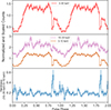 |
Fig. 3. Top: 3–30 keV pulse profile measured by NuSTAR. Middle: Hard (10–30 keV, purple) and soft (3–10 keV, orange) pulse profiles, scaled and normalized for clarity. Bottom: phase-resolved hardness ratio between the hard and soft pulse profiles. |
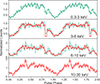 |
Fig. 4. Energy-resolved pulse profiles measured with NuSTAR (red) and XMM-Newton-pn (green). The pulse profile shape varies with energy. The sharp dip around ϕ = 0.85 in particular shows a strong dependence on energy, being most prominent in the 3–6 keV range. |
where Nmax is the value of the maximum bin for a given pulse profile, and Nmin is the value of the minimum bin. For all pulsed fraction calculations of the PFminmax estimator, we rebinned the profile into 25 bins to slightly smooth the profile. In order to account for background (e.g., non-source) contributions to the pulse profile, we simulated 1000 background-only pulse profiles given the total background counts measured for each energy bin. We subtracted these simulated background profiles from the measured pulse profile, weighting the background profile according to the difference in area between the source and background extraction regions. The result is 1000 hypothetical source-only pulse profiles. For each of these profiles, we then simulated 1000 iterations assuming Poisson statistics for each bin and calculated the resulting pulsed fraction. The mean of simulated pulsed fractions for each energy bin is shown in Figure 5, where uncertainties correspond to 1-σ confidence regions. For the 3–30 keV energy range, we find a pulsed fraction of  . Moreover, we find that the pulsed fraction increases with photon energy, reaching PFminmax = (94 ± 5)% in the hard X-ray range of 10–30 keV.
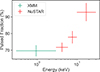 |
Fig. 5. Energy-resolved pulsed fraction PFminmax as measured by XMM-Newton (green) and NuSTAR (red). The pulsed fraction estimator exhibits a high overall value which strongly correlates with photon energy. |
Pulse profiles are characterized by a single-peak shape with a plateau spanning over half of the rotational phases at all energies, with the exception of a narrow dip around phase 0.85. To investigate the dip feature, we performed phase-resolved spectroscopy, extracting XMM-Newton and NuSTAR spectra within the bin 0.85 − 0.89 in phase. To fit the phase-resolved spectra, several different models can fit the data with comparable test statistic values due to the low statistics. None of them supports a significantly larger value of NH compared to the best-fit phase-averaged models. However, due to the low statistics, the results were inconclusive regarding the best-fit model and its best-fit parameters, which in several instances remained unconstrained.
5. Pulsed fraction spectra
We also investigated the dependence of the pulsed fraction on energy by employing the NuSTAR-tailored pipeline described in Ferrigno et al. (2023) (see also D’Aì et al. 2025; Maniadakis et al. 2025, for recent applications). This allows for optimal energy binning and computation of the pulsed fraction estimator that is not biased against extreme values or the number of bins (Antia et al. 2021). In this pipeline, pulse profiles are initially extracted in energy intervals corresponding to the intrinsic energy resolution of the NuSTAR FPM detectors and folded using a predefined number of phase bins (Nbins). The profiles are then dynamically rebinned to achieve a minimum signal-to-noise ratio (S/N ≳ 6) per pulse profile.
Once the rebinned profiles are obtained, the pulsed fraction is computed following the root-mean-square definition (PFrms, see Eq. (A.3) in Ferrigno et al. 2023). The associated uncertainties are estimated through a bootstrap procedure, in which 103 synthetic Monte Carlo profiles with the same statistical properties as the original data are generated and analyzed. We refer to the resulting dataset of energy-resolved PFrms values as the pulsed fraction spectrum (PFS), owing to its similarity to energy spectra in revealing local spectral features. To search for such features, we fit the PFS using a least-squares procedure with a polynomial function, increasing the polynomial degree until an adequate fit was obtained (see Ferrigno et al. 2023 for more details). All polynomial coefficients were treated as free parameters.
To investigate the dependence of the PFrms on both energy and the accretion regime, we also applied the same analysis to two additional NuSTAR observations previously presented in Pike et al. (2023) that sample the 2022 outburst at different stages (ObsID 80801347002 and 90801321001). Because the energy-resolved profiles are characterized by different statistical qualities and signal-to-noise ratios (S/N), the energy range over which reliable measurements of the PFrms can be obtained varies among observations. To achieve an optimal balance between energy resolution and well-constrained PFrms values, different phase-binning schemes and S/N thresholds were adopted depending on the data quality. For the observation with the highest statistics (ObsID 80801347002), we used 32 phase bins and a minimum S/N of 8. For the two remaining observations (ObsIDs 90801321001 and 31001020002), we employed 12 phase bins and a minimum S/N of 6. This strategy also defines the maximum usable energy range: for the lower S/N observations, PF measurements in the highest energy bins are affected by large uncertainties and were therefore excluded from the fit, limiting the PFS energy band to approximately 16 keV.
Our results are reported in Fig. 6, where we show the PFS and the best-fitting results for the three NuSTAR observations. The PFS of ObsID 80801347002 shows a clear energy dependence, characterized by a smooth increase from low to high energies. No clear feature indicative of a cyclotron line is observed at 44 keV or at other energies. On the other hand, a pronounced dip is observed in the PFS around the iron line energy band. By modeling this feature with a simple Gaussian absorption profile, we obtained a best-fitting centroid energy of 6.20 ± 0.05 keV and a width of 0.35 ± 0.06 keV (1σ c.l.). Remaining residuals following the fit suggest that the feature may have a more complex structure than that captured by a single Gaussian component. This, combined with the source falling near the detector edge, is likely the cause of the 6.4 keV iron line energy shift.
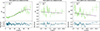 |
Fig. 6. Pulsed fraction spectra (see Sect. 5) of the three NuSTAR observations of MAXI J0655 taken during the 2022 outburst (ObsID 80801347002 and 90801321001), and in 2024 during the low-luminosity regime (ObsID 31001020002). Upper panels show data and a best-fitting polynomial fit. Lower panels show residuals in units of sigma with respect to the best fitting model. Note for the ObsID 80801347002 the presence of an additional Gaussian absorption line at ∼6.2 keV. For the other two observations the fit linear slope is consistent with zero at the 2σ c.l. |
The PFS of the two low-luminosity observations exhibits similar shapes, although they can be well described only up to ∼20 keV. No significant energy dependence of the PFrms is observed within this range, as the fit linear slope is consistent with zero at the 2σ c.l. in both cases.
6. Discussion
6.1. The double-hump spectrum
A double-hump spectrum in XRPs has been previously observed in GX 304-1 (Tsygankov et al. 2019b), A 0535+262 (Tsygankov et al. 2019a), GRO J1008-57 (Lutovinov et al. 2021), and very recently also in 2RXP J130159.6-635806 (Salganik et al. 2025) during the low-luminosity regime at ∼1034 erg s−1. A similar phenomenon has also been observed for X-Per at ∼1035 erg s−1 (Doroshenko et al. 2012). Recently, such a spectral shape has been modeled as the result of two distinct components, i.e., the low-energy “thermal” hump, dominated by photons with extraordinary polarization coming from deeper atmospheric layers (as they are scattered less frequently than ordinary photons), while the high-energy component is due to resonant Comptonization in the top heated layer of the atmosphere (Sokolova-Lapa et al. 2021). Based on the latter work, Zalot et al. (in prep.) are currently working on an alternative approach to estimating the magnetic field strength by using the position of the high-energy component of the double-humped spectrum. Their preliminary estimate of the magnetic field strength is in agreement with the lower end of the range proposed by Pike et al. (2023).
Our data do not allow us to appreciate any high-energy spectral curvature at the end of the observed bandpass (such an impediment is, in fact, encountered for most of the sources observed in the low-luminosity regime; see, e.g., GRO J1008-57, A 0535+262, 2RXP J130159.6-635806). On the other hand, there are cases where a double-hump spectral shape at low-luminosity is not observed altogether, that is, Swift J0243.6+6124 and MAXI J0903-531 (Doroshenko et al. 2020; Tsygankov et al. 2022, respectively). At least for the case of MAXI J0903-531, the absence of a double-hump spectrum at low-luminosity was interpreted in terms of a relatively low magnetic field, which would shift the high-energy bump, typically appearing around the cyclotron line centroid energy, into the bandpass of the low-energy bump, thus observationally merging with it. We nonetheless note that, in the case of our observations of MAXI J0655, the best-fit model is the one consisting of two distinct CompTT components, and that its best-fit spectral parameters (see Table 2) are in agreement with those observed in other sources whose data coverage or quality is such that the high-energy curvature is evident in their spectral shape (e.g., GX 304-1 and X-Per). The temperature of the seed photons, T0 ≈ 0.8 keV, is in agreement with that measured for other sources in the low-luminosity regime (Tsygankov et al. 2019a). The plasma temperature kT of the thermal and hot components, 1.8 keV and 21.5 keV respectively, is also in agreement with the values obtained from the other sources of reference (Tsygankov et al. 2019a,b), although the value of the hot component is consistent with that found in other sources mainly due to its high uncertainty. On the other hand, the plasma optical depth of the hot CompTT component tends to span an order of magnitude among the observed sources, with values that are often unconstrained and typically ≳10. On the contrary, for MAXI J0655 we obtain  , which is consistent with the value obtained for GRO J1008-57 in the low-luminosity regime (Lutovinov et al. 2021). The plasma temperature of the Hot Comptonized component is nominally high but has an unconstrained upper limit. At face value, this parameter indicates the over-heating of the upper atmospheric layers. In this regard, we notice that a fit with a frozen value of τp = 100 for the hot CompTT component (similarly to Salganik et al. 2025) returns a test statistic comparable to the model where the same component was allowed to vary during the fit procedure. Fixing the plasma optical depth value results in a well constrained plasma temperature of
  keV. This value is consistent with that observed in the above-mentioned works within 1σ. However, we also notice here that such a high value of the optical depth does not reflect our current understanding of the NS atmosphere, especially in the low-accretion regime. Moreover, depending on the electron density, it is expected that a plasma with such a high optical depth will reach thermal equilibrium, where a blackbody-like spectrum forms (Sokolova-Lapa et al. 2021). Such a fit should therefore be treated in a purely phenomenological way.
6.2. Discrete spectral features
Our XMM-Newton+NuSTAR spectral analysis shows no clear evidence of a cyclotron resonant scattering feature or an iron Kα emission line. In contrast, those features were observed in the XRPs A 0535+262 (Tsygankov et al. 2019a) and GRO J1008-57 (Lutovinov et al. 2021), respectively. However, we find evidence of an iron line in our PFS analysis (see Sects. 5 and 6.4 for a discussion). Pike et al. (2023) also do not find any spectral evidence of an emission iron line, but find hints of a spectral absorption feature that they tentatively interpret as a cyclotron line at 44 keV. In this regard, the CompTT + gabs model from Table 2 fits our data, but there is no evidence from previous observations of an absorption feature around 18 keV. A centroid energy of 18.3 keV would require a harmonic ratio of 2.4 to be interpreted as the fundamental line of the absorption feature hint observed by Pike et al. (2023) at 44 keV. Non harmonically spaced cyclotron line energies have been theoretically expected and observed in other sources, with a factor of up to about 30% difference from the 1 : 2 ratio (Nishimura 2005; Schönherr et al. 2007; Fürst et al. 2014). However, considering the luminosity-dependence shown by cyclotron line sources (see, e.g., Staubert et al. 2007; Malacaria et al. 2015; Klochkov et al. 2011), a luminosity change of a factor of 10 implies a change in the centroid energy of the cyclotron line of about 15%. On the other hand, the luminosity value measured during the observation where the hint of a cyclotron line at 44 keV was found is ∼5 × 1036 erg s−1 (Pike et al. 2023), while the luminosity value from our analysis is ∼5 × 1033 erg s−1. If the luminosity-dependence follows the above-mentioned trend, a factor of 103 in luminosity would therefore imply a shift in the cyclotron line centroid energy that is three times larger (i.e., 45%), which would bring the line to about 24 keV. This is significantly different from the Gaussian centroid best-fit energy of  keV (at a 90% c.l.). Moreover, we notice that the width and depth that we measure for the absorption feature (
 keV and
  keV, respectively) are typical of cyclotron lines (Staubert et al. 2019), although the large errors are likely indicative that the model is not appropriate. For these and more reasons (see Sects. 6.3 and 6.4), we disfavor the interpretation of the CompTT*gabs spectral model as an indication of the presence of a cyclotron line in MAXI J0655.
6.3. Timing results
In our low-luminosity observations of MAXI J0655 we measured a spin period of about 1081.86 ± 0.02 s. This is lower than the spin period measured by Pike et al. (2023) of 1085 ± 1 s (at 90% c.l.) obtained during the giant outburst in 2022. The spin derivative between those two measurements is −(4.6 ± 1.5)×10−8 s s−1. This implies that the source has been spinning up since the last outburst. This is consistent with the interpretation of the source belonging to the class of persistent BeXRBs (Reig & Roche 1999), characterized by low persistent X-ray luminosity, long (≳200 s) spin periods, and absent or weak iron emission lines in their X-ray spectrum (Reig 2011). In this regard, we point out that MAXI J0655 had been previously detected by SRG/ART-XC (Sunyaev et al. 2021; Pavlinsky et al. 2022; Sazonov et al. 2024) at a 4–12 keV flux of ∼7 × 10⁻¹² erg cm−2 s−1 (LX ∼ 1034 erg s−1), indicating that the source was already active at low luminosity outside the outburst. Moreover, assuming balance between the accretion torque  at the corotation radius, Rcor, and the angular momentum evolution,
  , then the measured spin period derivative corresponds to a value of the X-ray flux due to residual accretion of about ∼3 × 10⁻¹¹ erg cm−2 s−1. At a distance of 3.6 kpc, this corresponds to a luminosity of ∼4 × 1034 erg s−1, which is larger than the luminosity observed in this work by XMM-Newton or NuSTAR by a factor of a few. This tension may indicate that the source has experienced strong, sporadic spin-up episodes that went unobserved during the period between the outburst in 2022 and our observations in 2024.
During the 2022 outburst, Pike et al. (2023) measured a local spin-up trend that they interpreted according to the torque accretion model by Ghosh & Lamb (1979). This allowed them to recover a magnetic field strength of about 5 × 10¹⁴ G. By applying the same method, we obtain, for the same magnetic field strength and employing the luminosity value measured by XMM-Newton-pn, a spin-up value of about −6.4 × 10⁻⁶ s s−1. This is about two orders of magnitude stronger compared to the value inferred above as the spin derivative between the end of the outburst in 2022 and our observations in 2024. Magnetic field measurements through torque models are, however, troubled by systematic uncertainty of the physical details of how matter couples to the magnetic field. The difference between the models of how the predicted spin-up is related to the magnetic field value becomes even more significant for low mass accretion rates (Stierhof et al. 2025). In this regime, simulations also show a deviation from the torque models, indicating a change in the coupling mechanism not captured by the models (e.g., Ireland et al. 2022, but scaled for T Tauri stars). This could explain the high value obtained for the magnetic field, which would further imply a large magnetospheric radius, with consequences for the accretion dynamics. In fact, the rotating magnetosphere acts as a centrifugal barrier once the mass accretion rate drops below a certain value, thus settling the source in the so-called propeller regime (Illarionov & Sunyaev 1975). The luminosity corresponding to the onset of the centrifugal barrier is (Stella et al. 1986; Campana et al. 2002):
 (1)
(1)
where M1.4 is the neutron star mass in units of 1.4 M⊙, R6 is the NS radius in units of 106 cm, P is the NS spin period in seconds, B12 is the magnetic field strength in units of 1012 G, while k is the coupling factor relating the magnetospheric radius for disk accretion to the Alfvén radius calculated for spherical accretion (usually assumed to be k = 0.5). Employing the above-mentioned value of the magnetic field strength and a spin period of 1082 s, a canonical NS mass of 1.4 M⊙ and a NS radius of 12 km, we obtain a propeller luminosity of about ∼1.6 × 1035 erg s−1. On the other hand, if the magnetic field strength value is derived from the supposed cyclotron line at 44 keV, then we obtain a propeller luminosity of about ∼1.8 × 1031 erg s−1.
These measurements span a wide range of luminosity values, also covering those obtained by Swift/XRT, at ∼2 × 1033 erg s−1. The latter was obtained from a best-fit spectrum that is consistent with a power-law, although a blackbody fit cannot be ruled out due to the poor statistics. If the luminosity observed by Swift/XRT was actually due to a power-law spectrum, it would be considered an indication of residual accretion (see, e.g., Tsygankov et al. 2016), thus implying that the source has not yet entered the propeller regime. However, given that the available statistics prevent us from drawing such a conclusion, and because we cannot estimate the pulsating nature of the source at the time of the Swift/XRT observation, we conservatively adopt the XMM-Newton-pn luminosity (LXMM ∼ 5.8 × 1033 erg s−1, see Sect. 3) as the upper limit for entering the propeller regime (that is Lprop ≲ LXMM). This, in turn, allows us to put an upper limit on the magnetic field strength (see Eq. (1)) as B ≲ 8.9 × 10¹³ G.
6.4. Pulse profiles and pulsed fraction
We obtained energy-resolved pulse profiles for MAXI J0655 as observed at the low-luminosity stage. These differ from the pulse profiles observed during the outburst (Pike et al. 2023). In fact, during the 2022 outburst, the pulse profiles observed at an unabsorbed source luminosity of ∼6 × 1036 erg s−1 showed a double- or even triple-peaked shape at energies below 10 keV and a single-peaked structure at higher energies. On the other hand, at a lower luminosity of ∼7 × 1034 erg s−1 the pulse profiles became simpler at all energies yet showed signs of a double-peaked structure. The observed pulsed fractions at the two different luminosity stages were measured (for the full 3–78 keV energy range) as 84.4%±0.7% and 63%±6%, respectively. On the contrary, here we observe a pulse profile that is overall single-peaked at all energies, with a plateau structure spanning roughly 50% of the rotational phase. Additionally, we observe a short and sharp drop in counts around phase ϕ = 0.85 which is mostly apparent in soft X-rays. The dip is coincident in phase with a spike in the hardness ratio between 3–10 keV and 10–30 keV energy range.
The sharp phase- and energy-dependent dip around ϕ = 0.85 is similar to a feature in the pulse profile of EXO 2030+375 reported by Ferrigno et al. (2016), Fürst et al. (2017) and later observed again by Thalhammer et al. (2024). Ferrigno et al. (2016), Fürst et al. (2017) attributed this feature to increased absorption due to the self-occultation of the emitting region by part of the accretion column. Caballero et al. (2013) also observe a dip in the energy-resolved pulse profile of A 0535+26 below ∼20 keV during the decay of an outburst, at a 20–100 keV luminosity of about 3 × 1035 erg s−1. A similar feature was also observed in the soft energy pulse profile of the XRP RX J0440+4431 (Usui et al. 2012) and was likewise interpreted as being due to absorption from the accretion stream intercepting the line of sight during the NS rotation (Galloway et al. 2001; Malacaria et al. 2024; Salganik et al. 2023). Following this scenario, we may estimate the size of the occluding structure. Given a canonical neutron star radius of 12 km and a duration of the dip of about 4% of the spin period, we infer that the occluding structure size, if it consists of a region projected onto the NS, would be about 3.0 km. However, we also notice that, given the observed low-luminosity stage, it is unlikely that a column structure dense enough to produce the observed dip is present. Moreover, if the dip were solely due to absorption from neutral matter, then it would appear more pronounced at lower energies compared to the harder X-ray bands explored. This is not the case, as shown by the comparison of the pulse profiles in Fig. 4, where the dip appears most prominently in the 3–6 keV band instead of the 0.3–3 keV band. A possible influencing factor can be the presence of partially ionized material, which is characterized by only a weak dependence on photon energy and can be approximated by the Thomson scattering cross section. Alternatively, the soft (≲3 keV) emission is originating from an unabsorbed region.
Although no timing results are reported for most of the above-mentioned sources observed in the low-luminosity regime, for GRO J1008-57 the 3–79 keV pulsed fraction (measured as PFminmax) observed at ∼4 × 1034 erg s−1 is rather low, i.e., on the order of 20% (Lutovinov et al. 2021). For the persistent low-luminosity source X-Per, we also infer a PFminmax of about 50% in the 4–11 keV range from the RXTE pulse profiles obtained by Coburn et al. (2001). Jaisawal et al. (2021) also observed pulsations from EXO 2030+375 at a luminosity of about 2.5 × 1035 erg s−1, but with a relatively low PFminmax of less than 20% up to 80 keV. However, for MAXI J0655 we obtain an energy-dependent PFminmax that goes up to about 100% in the 10–30 keV energy band. Such a high pulsed fraction is observed in some sources only in the harder energy bands (≳50 keV, Lutovinov & Tsygankov 2009). Among them, we mention a few exemplary cases, such as SMC X-3 (Tsygankov et al. 2017), RX J0440.9+4431 (Liu et al. 2023), 2S 1417-624 (Liu et al. 2024). However, although the luminosity-dependence of the pulsed fraction in those sources is not clear, we notice that all of them show high values of the pulsed fraction at luminosities that are relatively high (greater than ∼1036 erg s−1) or even super-Eddington, and therefore at a substantially different accretion regime. On the contrary, there is no clear indication of any XRPs showing a ∼100% PFminmax in the energy range and luminosity regime considered in this work. It is not clear how such a high pulsed fraction can be produced. A possible qualitative scenario includes the idea that the hot spots responsible for the observed radiation are geometrically positioned in such a way that, at certain rotational phases, their emission is fully eclipsed from the observer line of sight. This is facilitated in the case, e.g., of a single spot emission. However, we also notice that the flat top pulse profile is not typical of single spot emission, thus implying that more complicating factors are at work.
The PFS obtained via the PFrms evolution with energy and luminosity highlights several spectral properties. First, a Gaussian feature corresponding to the iron Kα line at 6.4 keV has emerged at high luminosity. This is interesting, as persistent BeXRBs are characterized by weak or absent iron emission lines in their energy spectra. However, PFS has demonstrated the capability to uncover features that are hidden in the energy spectra (see, e.g., Ambrosi et al. 2025). The same line is not present in the PFS retrieved at lower luminosity, although low statistics prevent us from drawing firm conclusions. Moreover, PFS is a powerful tool for characterizing cyclotron lines by constraining both the centroid energy and the width of such features. Nonetheless, our analysis of the PFS does not show clear hints of the possible cyclotron line feature indicated by Pike et al. (2023) at 44 keV. This supports the interpretation that such a feature is, in fact, absent in the energy spectrum. The PFrms energy-dependence shows a flat trend (around 60%), which is contrary to what is observed from MAXI J0655 and other sources at higher luminosity. This might be due to the fact that photons from all probed energies originate in the same region and undergo the same pulsating mechanisms. Finally, we also notice that no appreciable features are present in the PFS obtained from our low-luminosity regime observation around the 3–6 keV energy range, where the pulse profile dip is more pronounced.
7. Conclusions
We observed the accreting XRP MAXI J0655 during its low-luminosity accretion regime with XMM-Newton and NuSTAR. We obtained broadband spectra and energy-resolved pulse profiles for the first time in this regime for this source. Our main findings can be summarized as follows:
-
The joint XMM-Newton+NuSTAR spectrum is best fit with a double-hump model. This is consistent with predictions that, at low luminosity, foresee the first hump peaking around 5 keV due to extra-ordinary polarization escaping from the lower layers of the atmosphere, while the higher energy hump peaks around 30 keV due to Comptonization by the top layers of the atmosphere over-heated by the residual accretion.
-
We measure a spin period of 1081.86 ± 0.02 s. This implies a spin-up compared to observations of MAXI J0655 taken in 2022 during an outburst episode. Therefore, the source has been accreting since then, instead of entering the propeller regime, thus supporting the identification of the source as a persistent BeXRB, and yielding an upper limit for the magnetic field strength of B ≲ 9 × 10¹³ G.
-
We obtain energy-resolved pulse profiles and observe an overall single-peaked profile with a plateau spanning roughly half of the rotational phase. This is markedly different from the profiles observed during the high-luminosity state obtained during the 2022 outburst. Moreover, the profiles show a narrow, sharp dip coincident with a spike in the hardness ratio, thus ascribable, at least in part, to increased absorption.
-
We measure different estimators of the pulsed fraction. The PFminmax shows an energy-dependent pulsed fraction that rises to about 100% in the 10–30 keV band. This is not observed in other sources, especially in such a low-luminosity regime. We also obtain PFrms and pulsed fraction spectra for MAXI J0655 at different luminosity stages. These show a flat energy-dependence at low luminosity, and the PFS obtained at high luminosity indicates the presence of an iron Kα emission line at 6.4 keV.
-
Detection of a cyclotron line is not supported by our spectral analysis, nor by the NuSTAR PFS obtained at high luminosity.
Acknowledgments
This work was supported by INAF (Research Large Grant FANS and GO Grant PULSE-X, PI: Papitto), the Italian Ministry of University and Research (PRIN MUR 2020, Grant 2020BRP57Z, GEMS, PI: Astone), and Fondazione Cariplo/Cassa Depositi e Prestiti (Grant 2023-2560, PI: Papitto). LD acknowledges funding from the Deutsche Forschungsgemeinschaft (DFG, German Research Foundation) – Projektnummer 549824807. RA acknowledges financial support from INAF through the grant “INAF-Astronomy Fellowships in Italy 2022 – (GOG)”. JBC is partially supported by NASA under award number 80GSFC21M0006.
References
- Ambrosi, E., D’Aì, A., Cusumano, G., et al. 2025, A&A, submitted [Google Scholar]
- Antia, H. M., Agrawal, P. C., Dedhia, D., et al. 2021, JApA, 42, 32 [Google Scholar]
- Arnaud, K. A. 1996, ASP Conf. Ser., 101, 17 [Google Scholar]
- Becker, P. A., & Wolff, M. T. 2022, ApJ, 939, 67 [NASA ADS] [CrossRef] [Google Scholar]
- Buccheri, R., Bennett, K., Bignami, G. F., et al. 1983, A&A, 128, 245 [NASA ADS] [Google Scholar]
- Caballero, I., & Wilms, J. 2012, Mem. Soc. Astron. Ital., 83, 230 [Google Scholar]
- Caballero, I., Pottschmidt, K., Marcu, D. M., et al. 2013, ApJ, 764, L23 [Google Scholar]
- Campana, S., Stella, L., Israel, G. L., et al. 2002, ApJ, 580, 389 [NASA ADS] [CrossRef] [Google Scholar]
- Cash, W. 1979, ApJ, 228, 939 [Google Scholar]
- Coburn, W., Heindl, W. A., Gruber, D. E., et al. 2001, ApJ, 552, 738 [NASA ADS] [CrossRef] [Google Scholar]
- D’Aì, A., Maniadakis, D. K., Ferrigno, C., et al. 2025, A&A, 694, A316 [NASA ADS] [CrossRef] [EDP Sciences] [Google Scholar]
- Deeter, J. E., Boynton, P. E., & Pravdo, S. H. 1981, ApJ, 247, 1003 [NASA ADS] [CrossRef] [Google Scholar]
- Doroshenko, V., Santangelo, A., Kreykenbohm, I., & Doroshenko, R. 2012, A&A, 540, L1 [NASA ADS] [CrossRef] [EDP Sciences] [Google Scholar]
- Doroshenko, V., Zhang, S. N., Santangelo, A., et al. 2020, MNRAS, 491, 1857 [Google Scholar]
- Evans, P. A., Beardmore, A. P., Page, K. L., et al. 2009, MNRAS, 397, 1177 [Google Scholar]
- Evans, P. A., Page, K. L., Osborne, J. P., et al. 2020, ApJS, 247, 54 [Google Scholar]
- Ferrigno, C., Pjanka, P., Bozzo, E., et al. 2016, A&A, 593, A105 [NASA ADS] [CrossRef] [EDP Sciences] [Google Scholar]
- Ferrigno, C., D’Aì, A., & Ambrosi, E. 2023, A&A, 677, A103 [NASA ADS] [CrossRef] [EDP Sciences] [Google Scholar]
- Fürst, F., Pottschmidt, K., Wilms, J., et al. 2014, ApJ, 780, 133 [Google Scholar]
- Fürst, F., Kretschmar, P., Kajava, J. J. E., et al. 2017, A&A, 606, A89 [NASA ADS] [CrossRef] [EDP Sciences] [Google Scholar]
- Gaia Collaboration (Vallenari, A., et al.) 2023, A&A, 674, A1 [NASA ADS] [CrossRef] [EDP Sciences] [Google Scholar]
- Galloway, D. K., Giles, A. B., Wu, K., & Greenhill, J. G. 2001, MNRAS, 325, 419 [NASA ADS] [CrossRef] [Google Scholar]
- Ghosh, P., & Lamb, F. K. 1979, ApJ, 234, 296 [Google Scholar]
- Huppenkothen, D., Bachetti, M., Stevens, A. L., et al. 2019, J. Open Source Softw., 4, 1393 [NASA ADS] [CrossRef] [Google Scholar]
- Illarionov, A. F., & Sunyaev, R. A. 1975, A&A, 39, 185 [NASA ADS] [Google Scholar]
- Ireland, L. G., Matt, S. P., & Zanni, C. 2022, ApJ, 929, 65 [NASA ADS] [CrossRef] [Google Scholar]
- Jaisawal, G. K., Naik, S., Gupta, S., et al. 2021, JApA, 42, 33 [Google Scholar]
- Kaastra, J. S., & Bleeker, J. A. M. 2016, A&A, 587, A151 [NASA ADS] [CrossRef] [EDP Sciences] [Google Scholar]
- Kang, J., & Wang, J. 2024, JUSTC, 54, 0702 [Google Scholar]
- Kennea, J. A., Evans, P. A., & Negoro, H. 2022, ATel, 15561, 1 [Google Scholar]
- Klochkov, D., Staubert, R., Santangelo, A., Rothschild, R. E., & Ferrigno, C. 2011, A&A, 532, A126 [NASA ADS] [CrossRef] [EDP Sciences] [Google Scholar]
- Liu, Q., Santangelo, A., Kong, L. D., et al. 2024, A&A, 691, A215 [NASA ADS] [CrossRef] [EDP Sciences] [Google Scholar]
- Liu, W., Reig, P., Yan, J., et al. 2023, arXiv e-prints [arXiv:2311.13844] [Google Scholar]
- Lutovinov, A., Tsygankov, S., Molkov, S., et al. 2021, ApJ, 912, 17 [Google Scholar]
- Lutovinov, A. A., & Tsygankov, S. S. 2009, Astron. Lett., 35, 433 [NASA ADS] [CrossRef] [Google Scholar]
- Madsen, K. K., Forster, K., Grefenstette, B. W., Harrison, F. A., & Miyasaka, H. 2021, arXiv e-prints [arXiv:2110.11522] [Google Scholar]
- Malacaria, C., Klochkov, D., Santangelo, A., & Staubert, R. 2015, A&A, 581, A121 [NASA ADS] [CrossRef] [EDP Sciences] [Google Scholar]
- Malacaria, C., Huppenkothen, D., Roberts, O. J., et al. 2024, A&A, 681, A25 [NASA ADS] [CrossRef] [EDP Sciences] [Google Scholar]
- Maniadakis, D. K., Sokolova-Lapa, E., D’Aì, A., et al. 2025, A&A, 700, A70 [NASA ADS] [CrossRef] [EDP Sciences] [Google Scholar]
- Mushtukov, A., & Tsygankov, S. 2022, arXiv e-prints [arXiv:2204.14185] [Google Scholar]
- Mushtukov, A. A., Suleimanov, V. F., Tsygankov, S. S., & Portegies Zwart, S. 2021, MNRAS, 503, 5193 [Google Scholar]
- Nagase, F. 1989, PASJ, 41, 1 [NASA ADS] [Google Scholar]
- Nakajima, M., Kohara, J., Serino, M., et al. 2022, ATel, 15453, 1 [Google Scholar]
- Nishimura, O. 2005, PASJ, 57, 769 [NASA ADS] [Google Scholar]
- Pavlinsky, M., Sazonov, S., Burenin, R., et al. 2022, A&A, 661, A38 [NASA ADS] [CrossRef] [EDP Sciences] [Google Scholar]
- Pike, S. N., Sugizaki, M., Eijnden, J. V. D., et al. 2023, ApJ, 954, 48 [Google Scholar]
- Reig, P. 2011, Ap&SS, 332, 1 [Google Scholar]
- Reig, P., & Roche, P. 1999, MNRAS, 306, 100 [NASA ADS] [CrossRef] [Google Scholar]
- Reig, P., Tzouvanou, A., & Pantoulas, V. 2022, ATel, 15612, 1 [Google Scholar]
- Salganik, A., Tsygankov, S. S., Doroshenko, V., et al. 2023, MNRAS, 524, 5213 [NASA ADS] [CrossRef] [Google Scholar]
- Salganik, A., Tsygankov, S. S., Chernyakova, M., Malyshev, D., & Poutanen, J. 2025, A&A, 698, A71 [NASA ADS] [CrossRef] [EDP Sciences] [Google Scholar]
- Sazonov, S., Burenin, R., Filippova, E., et al. 2024, A&A, 687, A183 [NASA ADS] [CrossRef] [EDP Sciences] [Google Scholar]
- Schönherr, G., Wilms, J., Kretschmar, P., et al. 2007, A&A, 472, 353 [NASA ADS] [CrossRef] [EDP Sciences] [Google Scholar]
- Serino, M., Negoro, H., Nakajima, M., et al. 2022, ATel, 15442, 1 [Google Scholar]
- Shidatsu, M., Pike, S., Mihara, T., et al. 2022, ATel, 15495, 1 [Google Scholar]
- Sokolova-Lapa, E., Gornostaev, M., Wilms, J., et al. 2021, A&A, 651, A12 [NASA ADS] [CrossRef] [EDP Sciences] [Google Scholar]
- Staubert, R., Shakura, N. I., Postnov, K., et al. 2007, A&A, 465, L25 [NASA ADS] [CrossRef] [EDP Sciences] [Google Scholar]
- Staubert, R., Trümper, J., Kendziorra, E., et al. 2019, A&A, 622, A61 [NASA ADS] [CrossRef] [EDP Sciences] [Google Scholar]
- Stella, L., White, N. E., & Rosner, R. 1986, ApJ, 308, 669 [Google Scholar]
- Stierhof, J. J. R., Sokolova-Lapa, E., Berger, K., et al. 2025, A&A, 698, A308 [NASA ADS] [CrossRef] [EDP Sciences] [Google Scholar]
- Sunyaev, R., Arefiev, V., Babyshkin, V., et al. 2021, A&A, 656, A132 [NASA ADS] [CrossRef] [EDP Sciences] [Google Scholar]
- Thalhammer, P., Ballhausen, R., Sokolova-Lapa, E., et al. 2024, A&A, 688, A213 [NASA ADS] [CrossRef] [EDP Sciences] [Google Scholar]
- Titarchuk, L. 1994, ApJ, 434, 570 [NASA ADS] [CrossRef] [Google Scholar]
- Tsygankov, S. S., Lutovinov, A. A., Doroshenko, V., et al. 2016, A&A, 593, A16 [NASA ADS] [CrossRef] [EDP Sciences] [Google Scholar]
- Tsygankov, S. S., Doroshenko, V., Lutovinov, A. A., Mushtukov, A. A., & Poutanen, J. 2017, A&A, 605, A39 [NASA ADS] [CrossRef] [EDP Sciences] [Google Scholar]
- Tsygankov, S. S., Doroshenko, V., Mushtukov, A. A., et al. 2019a, MNRAS, 487, L30 [NASA ADS] [CrossRef] [Google Scholar]
- Tsygankov, S. S., Rouco Escorial, A., Suleimanov, V. F., et al. 2019b, MNRAS, 483, L144 [NASA ADS] [CrossRef] [Google Scholar]
- Tsygankov, S. S., Molkov, S. V., Doroshenko, V., et al. 2022, A&A, 661, A45 [NASA ADS] [CrossRef] [EDP Sciences] [Google Scholar]
- Usui, R., Morii, M., Kawai, N., et al. 2012, PASJ, 64, 79 [NASA ADS] [Google Scholar]
- Wilms, J., Allen, A., & McCray, R. 2000, ApJ, 542, 914 [Google Scholar]
All Tables
Best-fit parameters of MAXI J0655 data from XMM-Newton+NuSTAR observations for two different spectral models.
All Figures
|
Fig. 1. XMM-Newton (0.5–10 keV) and NuSTAR (4–79 keV) both at 100 s binning light curves of MAXI J0655. Count rates were rescaled according to model predictions and effective area accounting for the observed spectral energy distribution. |
| In the text | |
|
Fig. 2. Unfolded spectra from XMM-Newton pn, MOS 1, and 2 (black, red, and green, respectively) and NuSTAR FPMA and FPMB (blue and cyan, respectively) from the MAXI J0655 observations in the low-luminosity regime analyzed in this work. Dashed lines represent the two Comptonization components for each instrument. Bottom panel: residuals to the best-fit double-CompTT model. |
| In the text | |
|
Fig. 3. Top: 3–30 keV pulse profile measured by NuSTAR. Middle: Hard (10–30 keV, purple) and soft (3–10 keV, orange) pulse profiles, scaled and normalized for clarity. Bottom: phase-resolved hardness ratio between the hard and soft pulse profiles. |
| In the text | |
|
Fig. 4. Energy-resolved pulse profiles measured with NuSTAR (red) and XMM-Newton-pn (green). The pulse profile shape varies with energy. The sharp dip around ϕ = 0.85 in particular shows a strong dependence on energy, being most prominent in the 3–6 keV range. |
| In the text | |
|
Fig. 5. Energy-resolved pulsed fraction PFminmax as measured by XMM-Newton (green) and NuSTAR (red). The pulsed fraction estimator exhibits a high overall value which strongly correlates with photon energy. |
| In the text | |
|
Fig. 6. Pulsed fraction spectra (see Sect. 5) of the three NuSTAR observations of MAXI J0655 taken during the 2022 outburst (ObsID 80801347002 and 90801321001), and in 2024 during the low-luminosity regime (ObsID 31001020002). Upper panels show data and a best-fitting polynomial fit. Lower panels show residuals in units of sigma with respect to the best fitting model. Note for the ObsID 80801347002 the presence of an additional Gaussian absorption line at ∼6.2 keV. For the other two observations the fit linear slope is consistent with zero at the 2σ c.l. |
| In the text | |
Current usage metrics show cumulative count of Article Views (full-text article views including HTML views, PDF and ePub downloads, according to the available data) and Abstracts Views on Vision4Press platform.
Data correspond to usage on the plateform after 2015. The current usage metrics is available 48-96 hours after online publication and is updated daily on week days.
Initial download of the metrics may take a while.