| Issue |
A&A
Volume 706, February 2026
|
|
|---|---|---|
| Article Number | A352 | |
| Number of page(s) | 12 | |
| Section | Numerical methods and codes | |
| DOI | https://doi.org/10.1051/0004-6361/202557896 | |
| Published online | 24 February 2026 | |
Optimising gravitational-wave sky maps for pulsar timing arrays
1
Max-Planck-Institut für Radioastronomie,
Auf dem Hügel 69,
53121
Bonn,
Germany
2
School of Physics and Astronomy, Monash University,
Clayton
VIC
3800,
Australia
3
OzGrav: The ARC Centre of Excellence for Gravitational Wave Discovery,
Clayton
VIC
3800,
Australia
4
Jodrell Bank Centre for Astrophysics, University of Manchester, Department of Physics and Astronomy,
Alan-Turing Building, Oxford Street,
Manchester
M13 9PL,
UK
5
Department of Physics and Astronomy, Vanderbilt University,
2301 Vanderbilt Place,
Nashville,
TN
37235,
USA
6
OzGrav: The Australia Research Council Centre of Excellence for Gravitational Wave Discovery
★ Corresponding author: This email address is being protected from spambots. You need JavaScript enabled to view it.
Received:
29
October
2025
Accepted:
18
December
2025
Abstract
Context. Pulsar timing arrays (PTAs) have recently reported compelling evidence for the presence of a gravitational-wave background signal. Mapping the gravitational-wave background is key to understanding how it is formed, since anisotropy is a tracer for, for example, a supermassive black hole binary origin.
Aims. In this work we refine the frequentist regularised gravitational-wave mapping analysis developed in our previous work (as part of the MeerKAT PTA 4.5-year data release). We derive a point-spread function describing the angular resolution of a PTA.
Methods. We investigate how the point spread function changes for different PTA constellations and determine the best possible angular resolution achievable within our framework. Using simulated data, we demonstrate that previous methods do not capture the actual resolution - especially in regions of the sky with a high density of pulsars.
Results. We propose an improved scheme that accounts for a variable local resolution and test it using realistic simulations of the latest MeerKAT dataset. We demonstrate that we are able to identify a continuous gravitational wave signal in a region with good pulsar sky coverage with approximately a factor of two increase in significance compared to our previous method.
Key words: gravitational waves / methods: data analysis / methods: laboratory: atomic / methods: statistical / stars: black holes / pulsars: general
© The Authors 2026
 Open Access article, published by EDP Sciences, under the terms of the Creative Commons Attribution License (https://creativecommons.org/licenses/by/4.0), which permits unrestricted use, distribution, and reproduction in any medium, provided the original work is properly cited.
This article is published in open access under the Subscribe to Open model.
Open Access funding provided by Max Planck Society.
1 Introduction
The gravitational wave (GW) spectrum accessible with current and future observatories is commonly divided into three different regimes reflecting the observing band of these detectors. In contrast to the individually resolvable GWs in the intermediate-and high-frequency regime (> 10 μHz), the primarily targeted GW signal in the nanohertz regime is the gravitational wave background (GWB) (Rosado et al. 2015).
It is likely that this GWB is caused by the incoherent superposition of GWs emitted by the population of supermassive black hole binaries (Rajagopal & Romani 1995; Allen & Ottewill 1997). Supermassive black holes are thought to be found in centres of galaxies (Kormendy & Richstone 1995), and so a supermassive black hole binary is likely to form during a galaxy merger (Begelman et al. 1980). Historically, the inspiral of circular supermassive black hole binaries was expected to stall (‘final parsec problem’ Milosavljevic & Merritt 2003), but various theories have been put forward that allow the supermassive black holes to get so close that they become GW-driven (Holley-Bockelmann & Khan 2015; Gualandris et al. 2017; Ryu et al. 2018). Such a supermassive black hole binaryoriginating GWB would create an anisotropic distribution of GW power across the sky, once due to the finite number of supermassive black hole binaries contributing to the signal (Allen & Ottewill 1997; Mingarelli et al. 2013; Gair et al. 2014; Mingarelli et al. 2017), but also as it is expected that the supermassive black hole binary population follows the large-scale cosmic structure (Burke-Spolaor et al. 2019). Additionally, individual close-by ‘loud’ supermassive black hole binaries are expected to stand out from the quasi-isotropic background Sesana et al. (2004); Yardley et al. (2010); Sesana & Vecchio (2010), so-called hotspots.
A nanohertz GWB signal can also be caused by early-Universe processes (Maggiore 2000), such as phase transitions (Caprini et al. 2020; Hindmarsh et al. 2021), cosmic string collapse (Hindmarsh & Kibble 1995; Saikawa 2017), or primordial GWs from quantum fluctuations that were redshifted by inflation (Guzzetti et al. 2016; Lasky et al. 2016; Yuan & Huang 2021; Domènech 2021). For most of these models, the GWB is expected to be isotropic.
This makes the nanohertz GW regime interesting - either offering a unique window onto galaxy evolution studies and/or constraining processes in the early Universe. For nanohertz frequencies, a suitable GW detector needs to be galaxy-sized. This is realised in pulsar timing arrays (PTAs) (Sazhin 1978; Detweiler 1979). A PTA consists of a group of millisecond pulsars that are regularly monitored over years to decades, usually using radio telescopes. Gravitational wave detection with PTAs is based on the exceptional rotational stability of these pulsars. Due to the clock-like predictability of the pulse times-of-arrival (ToAs), even small-scale deviations caused by GWs can be detected. Pulsar timing residuals are obtained by subtracting the ToA prediction of the best-fitting timing model from the recorded ToAs. Residuals caused by GWs are then detected by searching for quadrupolar correlations across the residual series of all pulsars in the PTA. The stochastic GWB is characterised as a noisy red process (Allen & Romano 1999) that exhibits angular correlation according to the Hellings-Downs curve (Hellings & Downs 1983).
In recent years, different PTA collaborations have independently reported compelling evidence for the presence of such a GWB signal in their datasets (EPTA Collaboration and InPTA Collaboration 2023; Agazie et al. 2023a; Reardon et al. 2023; Miles et al. 2025b; Xu et al. 2023). Naturally, one of the next key steps is determining the origin of this signal. A key method of discriminating the different scenarios described above is calculating GW sky maps and determining the level of anisotropy across the sky map. A significant anisotropy is an indicator of an astrophysical GWB. Simultaneously, a hotspot is a smoking gun for the presence of an individually resolvable supermassive black hole binary, a signal that is yet to be detected in PTA datasets. Hence, the search for anisotropy is of increased interest to the PTA community and has gained significant momentum.
Based on the sky mapping methods built for ground- and space-based GW detectors (Mitra et al. 2008; Thrane et al. 2009; Banagiri et al. 2021), several approaches to obtain GW power sky maps from PTA data were developed. Those methods, both frequentist (Thrane et al. 2009; Pol et al. 2022; Grunthal et al. 2025) and Bayesian (Mingarelli et al. 2013; Taylor & Gair 2013; Cornish & van Haasteren 2014; Taylor et al. 2020), analyse and quantify the level of anisotropy by expanding the GW power in some choice of sky-resolving basis, and constraining the basis coefficients. The spherical harmonic expansion is used most widely, either linearly, or in form of the square-root spherical harmonics to ensure positivity of the recovered sky map. The application of these methods to real PTA datasets was performed in Taylor et al. (2015); Agazie et al. (2023b), and Grunthal et al. (2025), our recent anisotropy study as part of the MeerKAT PTA (MPTA) 4.5-year data release (Miles et al. 2025a). In that work we have presented a framework to characterise the anisotropy of the GWB that improved the spherical harmonic frequentist approach (Thrane et al. 2009; Pol et al. 2022) by installing a regularised maximum likelihood estimation that includes GWB self-noise.
A key point of calculating GW sky maps is to account for the diffraction limit of the PTA, caused by the limited number of pulsars used to construct the map. All recent works on PTA GW power map making (Romano & Cornish 2017 ; Agazie et al. 2023b; Grunthal et al. 2025) based on spherical harmonic expansions handle the diffraction limit of a PTA by imposing that the maximum number of spherical harmonics modes used in the expansion should not surpass the number of pulsars in the array. This approach treats the diffraction limit as a global problem, and in consequence introduces a globally defined maximum angular resolution of the resulting sky map. However, as was shown by Boyle & Pen (2012), the local resolving power of a PTA dataset strongly depends on the pulsar distribution across the sky. In addition, Floden et al. (2022) demonstrated that for Earth-based GW detectors the sky localisation of single sources can be improved by including higher-order spherical harmonics beyond ℓmax obtained from the diffraction limit argument. Thus, the ultimate aim of this follow-up work to Grunthal et al. (2025) is to improve the currently used regularised spherical harmonics expansion scheme such that it properly reflects the local resolution of the PTA, while respecting the global analysis limit imposed by the number of pulsars. We expect that the updated scheme also provides a more precise localisation of anisotropic structures in the map, which ultimately can optimise follow-up analyses (D’Orazio & Charisi 2023; Agarwal et al. 2026) and guide candidate vetting.
We begin by giving a brief introduction to PTA sky map analysis in Sect. 2. The first major result of our work is then presented in Sect. 3, in which we develop a mathematical framework to calculate the point spread function (PSF) of a PTA dataset analysed with a regularised spherical harmonics framework. We employ it to revisit the spherical harmonics expansion scheme using a hypothetical isotropic PTA, presented in Sect. 4. We first discuss two major shortcomings of the current expansion, and then present the improved expansion strategy allowing to overcome these, the second major result of this work. Finally, we test the reworked analysis set up utilising more realistic simulations of the MPTA 4.5-year dataset, and discuss the results in Sect. 5. We conclude with a summary and outlook in Sect. 6.
2 Methods
Our methods and notation closely follow our previous work Grunthal et al. (2025). Hence we only give a minimum self-consistent overview on the basics of PTA datasets and GW sky mapping from those in this work. We refer to Grunthal et al. (2025) and references therein for further details, especially on the mathematical intricacies of the method.
2.1 PTA datasets and the overlap reduction function
A PTA dataset is a collection of ToA time series,  , from Npsr pulsars, in which a GWB signal appears as an angularly correlated stochastic process. The ToAs are characterised by a multivariate normal distribution with a covariance matrix. The total noise budget of a PTA dataset is quantified in terms of the ToA covariance matrices:
 (1)
(1)
The auto-correlation part, Caa, describes the noise processes associated with each pulsar, whereas the cross-correlation matrix,
 (2)
(2)
depends only on the GW signal. Via the Fourier basis vectors,  , it is usually expressed in terms of the angular correlation coefficients, Γab (Allen & Ottewill 1997), and the diagonal Fourier domain covariance matrix,
 (3)
(3)
This matrix is built from the GWB power spectral density (PSD) S(fk), parametrised in terms of an amplitude, AGWB, and a spectral index, γGWB, as well as the frequency bin width, ∆f = 1/Tobs, where Tobs denotes the total time span of the dataset, and the normalising factor fyr = 1/1 yr. For the GWB it is expected that γGWB > 0, especially, if it originates from circularly inspiraling supermassive black hole binaries, γGWB = 13/3. A stochastic process with a PSD that rises at low frequencies is referred to as red noise. Since the GWB signal is common to all pulsars, this signal is said to produce a ‘common red noise’. Given the capabilities of current PTA datasets, we assume that the common red noise is completely described by the parameters AGWB and γGWB.
In the presence of a GW signal, the angular correlation function is given by the so-called overlap reduction function (Allen & Romano 1999; Mingarelli et al. 2013)
![Mathematical equation: \Gamma_{ab} \propto \int_{S^2} \! \mathrm{d}\Hat{\Omega} \; \mathcal{P}(\Hat{\Omega}) \left[ \mathcal{F}_a^+(\Hat{\Omega})\mathcal{F}_b^+(\Hat{\Omega}) + \mathcal{F}_a^\times(\Hat{\Omega})\mathcal{F}_b^\times(\Hat{\Omega})\right],](/articles/aa/full_html/2026/02/aa57896-25/aa57896-25-eq6.png) (4)
(4)
where P(Ω̂) is the probability density function for GW power at different locations on the sky, Ω̂, as calculated from the Solar system barycentre, and
 (5)
(5)
is the antenna factor for a GW with polarisation state A, propagating along the vector k̂, as measured by a pulsar located in the direction  . The term
  denotes the (i, j) components of the polarisation tensor for a GW with polarisation A, in the polarisation basis from, for example, Taylor et al. (2020).
Our goal is to obtain an estimate for P(Ω̂). To this end we express P(Ω̂) in terms of a suitable basis, so that the basis coefficients can be constrained with PTA data. Following Grunthal et al. (2025), we employed a spherical harmonic basis,
 (6)
(6)
with complex-valued spherical harmonics, Yℓm(Ω̂) weighted by real-valued coefficients, Pℓm (Cornish 2001; Kudoh & Taruya 2005; Cornish & van Haasteren 2014). Owing to the finite spatial resolution of a PTA, the sum truncates at an ℓmax value. The details of determining ℓmax are discussed in Sect. 4.
Using notation consistent with Grunthal et al. (2025), henceforth indices α and β denote pulsar pairs (ab); μ and ν denote spherical harmonics. We write the overlap reduction function using the Einstein summation convention as
![Mathematical equation: \Gamma_\alpha &= \int d\Omega \left[ \mathcal{F}^+_a(\hat\Omega) \mathcal{F}^+_b(\hat\Omega) + \mathcal{F}^\times_a(\hat\Omega) \mathcal{F}^\times_b(\hat\Omega)\right] Y_\mu(\hat\Omega) P_\mu \\](/articles/aa/full_html/2026/02/aa57896-25/aa57896-25-eq11.png) (7)
(7)
 (8)
(8)
where Rαμ is referred to as the ‘response matrix’.
2.2 Per-frequency pulsar pair cross-correlations
In the frequentist framework (Mitra et al. 2008; Thrane et al. 2009), the overlap reduction function is estimated from Npairs distinct pulsar pair cross-correlations, {ρα}, designed such that (Demorest et al. 2013; Chamberlin et al. 2015)
 (9)
(9)
Individual binaries are the most anticipated source of anisotropy (Sesana & Vecchio 2010; Cornish & van Haasteren 2014; Burke-Spolaor et al. 2019). As a single binary emits GWs in a narrow frequency band, PTA anisotropy studies aim to calculate narrowband sky maps at individual frequency bins of the PTA (Pol et al. 2022; Agazie et al. 2023b; Grunthal et al. 2025).
We calculated these maps from narrow-band pulsar pair cross-correlations, obtained from the narrow-band optimal statistic (Gersbach et al. 2025), implemented in the PYTHON package DEFIANT1. For the pulsar pair α at the kth frequency bin, the narrow-band pulsar pair cross-correlation is
![Mathematical equation: \rho_\alpha(f_k)\equiv \rho_{k,\alpha} = \frac{\Vec{X}_a^T\Tilde{\phi}(f_k)\Vec{X}_b}{\Tr\left[Z_a \Tilde{\phi}(f_k) Z_b \Phi(f_k) \right]},](/articles/aa/full_html/2026/02/aa57896-25/aa57896-25-eq14.png) (10)
(10)
where
 (11)
(11)
 (12)
(12)
The frequency selector matrix,
 (13)
(13)
encodes the frequency bin at which the cross-correlation is eval-uated2. The frequency-domain pulsar pair covariance matrix is normalised like so:
 (14)
(14)
ensuring that
 (15)
(15)
2.3 Sky map calculation in spherical harmonics decomposition
With the set of cross correlations, {ρk,α}, a GW sky map was obtained by calculating the coefficients, P′, that maximise the cross-correlation likelihood (Mitra et al. 2008; Thrane et al. 2009; Pol et al. 2022). The equations governing the sky map calculation (e.g. in Pol et al. 2022; Grunthal et al. 2025) hold for both a single frequency as well as broadband pulsar pair correlations, so adopting the notation introduced in Eq. (10), the likelihood reads
![Mathematical equation: {\cal L}\left(\Vec{\rho}_k | \Vec{P}_k\right) = \frac{\exp\left[-\frac{1}{2}\left(\Vec{\rho}_k - \mtx{R}\Vec{P}_k\right)^\dag \mtx{\Sigma}_k^{-1}\left(\Vec{\rho}_k - \mtx{R}\Vec{P}_k\right)\right]}{\sqrt{\det(2\pi\mtx{\Sigma}_k)}},](/articles/aa/full_html/2026/02/aa57896-25/aa57896-25-eq20.png) (16)
(16)
where Σk is the covariance matrix of the cross-correlations at the GW frequency fk. We included off-diagonal terms in Σk to take into account GW-induced pulsar-pair covariance (Allen & Romano 2023). The detailed expressions for the full matrix entries can be found in the appendices in Gersbach et al. (2025) and Grunthal et al. (2025).
The maximum likelihood estimator is given as (Mitra et al. 2008; Thrane et al. 2009; Pol et al. 2022; Grunthal et al. 2025)
 (17)
(17)
where the vector
 (18)
(18)
is known as the dirty map, i.e. an inverse-noise weighted representation of the GW power on the sky as seen through the response of the pulsars (Thrane et al. 2009; Pol et al. 2022; Agazie et al. 2023b; Ali-Haïmoud et al. 2021). Meanwhile,
 (19)
(19)
is the Fisher matrix of the maximum likelihood estimators.
Following the findings and arguments in Grunthal et al. (2025), we regularised the Fisher matrix inversion in Eq. (17). This was done with the singular value decomposition scheme outlined in Thrane et al. (2009); Abadie et al. (2011); Grunthal et al. (2025), whereby the first sreg sorted eigenvalues of M were kept, and beyond that threshold, the remaining smaller ones were set to infinity3. This accounts for the variations in the constraints of the different eigenmodes of M due to the sky distribution and sensitivity of the pulsars. The regularised maximum likelihood estimate is
 (20)
(20)
where  is the pseudo-inverse of Mk containing only the first sreg eigenmodes of Mk. The tildes denote regularised quantities. Choosing the number of modes to keep is a trade-off. By throwing out some modes, the sky map becomes biased because these rejected modes are no longer included in the sky maps. But on the other hand, we also remove poorly constrained modes that contribute only noise to the sky map.
In contrast to the dirty map, the maximum-likelihood estimators P′k and  (Eqs. (17) and (20)) are referred to as the clean map4. So in summary, calculating a frequentist GW sky map starts with obtaining the dirty map from the pulsar pair correlations and the Fisher matrix from the PTA noise models. Then, the regularised inverse of the Fisher matrix is calculated, and multiplied with the dirty map to obtain the regularised clean map.
The uncertainty associated with this regularised clean map is
 (21)
(21)
The clean map signal-to-noise ratio (S/N) is given by
 (22)
(22)
Here the subscript Ω̂ indicate that we have transformed the numerator and denominator from the spherical harmonic basis to the pixel basis.
In the following, we drop the subscript k and implicitly assume frequency resolved quantities. All other previously introduced conventions and notations remain unchanged.
3 Sky resolution of a PTA dataset
We demonstrated in our previous work that the sky map output from a PTA dataset depends on the data analysis scheme. Hence, a quantity measuring the resolving properties should reflect all aspects of the analysis, especially the influence of the regulari-sation scheme. Due to the anisotropic distribution of pulsars on the sky, it is natural to expect that the resolvability of a PTA varies with sky position; in regions with a high sky density of pulsars, we expect the PTA to resolve structure better than in regions sparsely populated with pulsars.
3.1 PTA point spread function
The resolution of an imaging tool can be characterised by its ability to resolve point sources, captured in the so-called PSF. In the context of GW astronomy, this corresponds to determining how a single GW point source at the sky position Ω̂i appears on the clean sky map after observing it with the method described in the previous section.
First, we have to choose a suitable representation of the point source. For a visualisation on a pixellated sky map, we transformed the spherical harmonics maximum likelihood solution, P, into its pixel basis representation, PΩ̂, via
 (23)
(23)
where U is a unitary basis transformation matrix. The centre of each pixel represents an (RA, DEC) co-ordinate pair, and the pixel size was chosen such that the smooth features of the spherical harmonics representation are properly displayed on the resulting sky map. A side effect of this fine-grained pixelation is that the pixel size is well below the average angular separation of two pulsars. Hence, we can model a GW point source located at Ωi with a single ‘hot’ pixel at that position. Using vector notation, a single hot pixel at the ith pixel position can be written as
 (24)
(24)
Capturing this hot pixel through the PTA leads to the dirty map
 (25)
(25)
where we have used Eq. (17), explicitly including the basis transformation.
In the usual anisotropy analysis, this dirty map is deconvolved with the regularised dirty map, M̃, to obtain the clean map. Hence, the full expression for the clean map representation of the hot pixel is given as
 (26)
(26)
This equation describes the recovered clean map under the assumption that the pulsar noise models are a perfect representation of the actual pulsar noise budget, i.e. M̃-1 and M contain the same noise values. In real PTA datasets, the clean map representation of a GW point source can be influenced by noise misspecification. For completeness, we provide a derivation and analysis of the full expression for the recovered clean map in Appendix A, which also accounts for an (assumed) noise misspecification. We also demonstrate that it recovers Eq. (26) in the limiting case of perfect pulsar noise models.
In Fig. 1, we show the transformation process due to the reg-ularisation using a single hot pixel observed through a simple PTA consisting of 40 pulsars equally distributed on the sphere using the Fibonacci lattice technique5. We can clearly see the blurring due to the regularisation taking place.
From this clean sky map, we can now calculate the value of the PSF at the ith pixel, Apsf,i, by determining the area to which a hot pixel is blurred out as
 (27)
(27)
where we defined the blurred area to include all pixels with values larger than half the maximum of the sky map.
In practice, APSF,i is calculated by normalising  by its maximum value, and adding up the areas of all pixels whose clean map values are larger than 0.5. The area of each pixel is obtained from the small area approximation on the sphere, ensuring that the sum of all pixel areas add up to 4π.
If this evaluation of the point spread area is done iteratively for all pixels, we obtain the PSF sky map, i.e. the point spread area as function of sky position. The values of the PSF map have units of areas.
Notably, this method allows for the addition of disjoint areas, as long as their PSF values are above the threshold. This, in turn, can lead to unreliable PSF estimates. Possible solutions could include an alternative effective-area definition, or imposing a connected-area condition on the PSF estimation. However, we determine that this failure mode happens rarely and only in areas with poor resolution where the GW power of the point source is spread out widely across the map, making the map maximum barely distinguishable from the noise floor. In areas with a reasonably high resolution, this issue does not arise. As the following work focuses on the sky areas in which the PTA has the best resolution, we defer mitigating this issue to a future work.
We note that in general a PSF features both an area as well as a location of a recovered point source. Investigating sky maps similar to Fig. 1, we also found that the sky position of the clean S ∕N map maximum does not always correspond to the sky position of injected the hot pixel. This behaviour is likely caused by superposition of antenna patterns from the pulsars. In areas densely populated by pulsars, there is little to no position offset along the connecting lines of next-neighbour pulsars, but a slight dislocation if the source is encircled by pulsars. This offset does not go beyond the area that is enclosed by the pulsars, and also falls into the PSF extent. For sources that are in an area with little to no pulsar population on a large scale, the S/N recovered from the source is close to the noise floor. This leads to large displacements, but in turn they are not associated with a source detection. So the PTA geometry and analysis pipeline can also introduce a mismatch between the actual and recovered source position. While this position distortion feature is of interest for identifying the host of a single supermassive black hole binary GW signals, and could be investigated further, for instance in the scope of a hotspot-galaxy-catalogue-crossmatching study, our focus remains on investigating the PSF area behaviour.
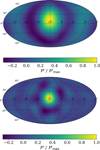 |
Fig. 1 Single hot pixel seen through a 40PSR PTA with different regularisation cut-offs. The crosshair indicates the position of the hot pixel. Top: clean map with ℓmax = 8, sreg = 15. Bottom: clean map with ℓmax = 8, Sreg = 40. |
3.2 The PTA distortion matrix
In order to find an efficient implementation of the PSF calculation scheme, we return to Eq. (26). Looking closer, we find that the multiplication with  is nothing but selecting the ith column of the matrix product
  , as
, as  can be interpreted as the canonical basis vectors of a Npix-dimensional Euclidean space. Conveniently, all quantities in Eq. (28) can be accessed as by-products of the existing sky map analysis framework. So, the calculation of the PSF due to the regularisation scheme becomes an iterative evaluation of the column vectors of
  .
.
Hence, this matrix holds all hot-pixel clean sky maps as its column vectors, and hence all information about the PSF. This motivates the defining of this matrix product as the Npix × Npix ‘distortion matrix’ of a PTA with a regularisation cut-off, sreg,
 (28)
(28)
The quantity ΛSreg is its spherical harmonics-space representation. Intuitively,  (or ΛSreg) contains all information about the smear that the PTA introduces to point-like GW sources, due to the regularisation of the Fisher matrix inversion.
Comparing Eq. (28) to the definition of the PTA clean sensitivity map, Eqs. (D2) and (D3) in Grunthal et al. (2025), we find that the sensitivity map is calculated from the main diagonal of  . This is not surprising, as both quantities share the underlying question of how a point source appears in the analysis product. The mathematical similarity demonstrates not only the closeness between these two methods, but also the importance of
  and ΛSreg, respectively, in the context of characterising a PTA.
Investigating ΛSreg from an algebraic point of view, we notice the following: rewriting it in terms of the singular value decomposition of M, M = VΞV† with the unitary matrix V, we arrive at
 (29)
(29)
 (30)
(30)
where  . Hence, ΛSreg is the orthogonal projector onto the regularised subspace, i.e. the subspace spanned by the first sreg left singular vectors of M. The quantity
  is the representation of this spectral projector in the pixel basis. As a consequence, the clean sky maps corresponding to the individual pixels are the column vectors of the spectral projector in the pixel basis. This is mathematically capturing the impact of the information loss due to the regularisation, required from the noise and geometry of the PTA.
4 Revisiting the current spherical harmonics scheme
The number of spherical harmonic modes, {(ℓ, m)}, that can be uniquely constrained cannot be larger than the number of pulsars. In the scheme currently employed for PTA sky map analyses (Pol et al. 2022; Agazie et al. 2023b; Grunthal et al. 2025), this is enforced by choosing  . We refer to this as the ‘classic scheme’. The disadvantage of this approach is that it does not take into account the fact that the resolution of a PTA often varies across the sky. We use the PSF maps developed in the previous section in order to allow for an adaptive scheme in which the resolution varies across the sky.
4.1 Shortcomings of the currently used (classic) scheme
For this investigation we simulated an artificial PTA consisting of 40 pulsars, isotropically distributed according to a Fibonacci lattice. All pulsars have a root mean square of 100 ns, regular ToAs over a total observation time span of 10 yr, and are simulated with white noise only. The analysed ToAs were simulated using LIBSTEMPO.
One expects that such a PTA should allow for 40 equally constrained spherical harmonics modes, since all pulsars contribute equally in this PTA, and they are isotropically distributed across the sky. But the classic scheme demands that ℓmax = 5, so the spherical harmonics expansion contains only 36 modes. Following the scheme leads to purposefully ignoring a subset of the constraints provided by the PTA dataset, although all of them are equivalent. One major consequence of this negligence becomes imminently accessible from the PSF map of this set-up (40 pulsars, ℓmax = 5, sreg = 35), shown in the top plot in Fig. 2. We would expect any pattern visible on the map to follow the position of the pulsars, as well as similar pulsar constellations to lead to similar PSF values. Yet, we find an irregular pattern that is not correlated with the pulsar positions. This is not expected and indicative of a sub-optimal set-up.
In the next step, we removed half of the pulsars in the 40 pulsar isotropic array with RA <12 hr. In the classic scheme, this would allow for a spherical harmonics expansion to ℓmax = 3. The corresponding PSF map of this set-up (20 pulsars, ℓmax = 3, sreg = 15) is shown in the lower plot of Fig. 2. The increased values of the PSF show that while we only reduced the number of pulsars in one particular part of the sky, we gave up on spatial resolution across the whole sky. Moreover, we would logically expect the resolution of the PTA on the part of the sky where the pulsars were not removed to be the same as for the full 40 pulsar PTA. As we can see from the PSF map, this is clearly not the case.
Thus, we have identified several shortcomings of the scheme currently used to set up spherical-harmonics-based anisotropy analyses. In the next step, we aim to mitigate these problems with a revised set-up procedure.
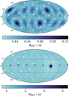 |
Fig. 2 Sky maps showing the (S/N-based) PSF of the PTA as a function of sky position. The white stars indicate the positions of the pulsars in the respective PTA. Both plots were calculated using the classic spherical harmonics expansion scheme based on the number of pulsars. Top: 40 pulsar PTA, ℓmax = 5, sreg = 35. Bottom: 20 pulsar subset PTA, ℓmax = 3, sreg = 15. |
4.2 An enhanced scheme for regularised gravitational-wave sky map calculation
It is clear that the current scheme of choosing ℓmax based on the number of pulsars neither reflects the actual PTA sky resolution nor is flexible enough to adapt to uneven pulsar constellations. Hence we propose a shift in the paradigm. We chose the maximum spherical harmonics degree, ℓmax, such that it reflects the pulsar distribution in the highest populated sky areas. The surplus modes, i.e. the over-resolution in sparsely populated sky areas, can then be removed using the established regularisation scheme.
The choice of sreg is a trade-off between including additional unspecified noise and rejecting signal information. It reflects the difference in the sensitivity of the individual pulsars, but also the lack of support of those spherical harmonics modes falling in sky areas with a local underdensity in the pulsar distribution. In a sense, the surplus modes are no different to those modes already regularised in the classic scheme. None of them is well constrained. With this approach, the condition that no more modes than the number of pulsars can be constrained translates into a limit on the regularisation cut-off, namely sreg ≤ NPSR.
 |
Fig. 3 Point spread area sky maps for the 40 pulsar isotropic PTA set-up. From left to right: ℓmax = {6,8,10,12}. The white stars indicate the pulsar positions. |
 |
Fig. 4 Point spread area sky maps for the 20-pulsar sub-array of the 40 pulsar isotropic PTA set-up. From left to right: ℓmax = {4,8,10,12}. The white stars indicate the pulsar positions. |
4.2.1 Creating credible PSF sky maps
We explore the effect of increasing ℓmax with the full 40 pulsar PTA. Due to the symmetries in the set-up, we set sreg = 40 and increased ℓmax. The resulting PSF maps are shown in Fig. 3. The improvement in both the minimum PSF values as well as the regularity of the pattern across the sky is directly visible.
For the larger values of ℓmax, we find that the pattern reflects the expectation from the single pulsar response (Romano & Allen 2024). The PSF is smaller in regions between four pulsars, but on connection lines between two adjacent pulsars it is larger, as only two pulsars constrain the source position.
This demonstrates that this approach allows us to model the PTA geometry more accurately. Moreover, we find that for ℓmax = {10,12} neither the range of the PSF values (range of the colour bar) nor the pattern on the map significantly changes. This is a first indication of some kind of convergence behaviour that can help to identify a suitable ℓmax.
Next we performed the same study on the 20 pulsar sub-array for ℓmax ∈ [4,12]. As we had 20 identical pulsars contributing to the array, we set sreg = 20. In Fig. 4 we show exemplary sky maps for ℓmax = {4,8,10,12}.
Similar to the full-array case, we find that the minimum PSF decreases with increasing ℓmax, and that it reaches some lower bound towards ℓmax = 12. We can also see that for ℓmax = {8,10,12} the same net-like pattern emerges as in the PSF sky maps of the full 40-pulsar PTA. More specifically, the pattern is visible on the left part of the sub-array sky maps, where the remaining 20 pulsars are located. This supports our expectation that the point source resolution of a PTA is dominated by the local pulsar constellation. Since on the left part of the map the full array and the sub-array locally follow the same constellation, the similar sky pattern demonstrates that our method suitably traces the PTA properties.
As a side note, we find that on the ℓmax = 4 sky map the PSF is seemingly smaller in the region with no pulsars than in the region densely populated with pulsars. Upon closer inspection, it turns out that this unintuitive result is an artefact of the area evaluation scheme, as is pointed out in Sect. 3.1. Due to the sparse pulsar population, the corresponding clean maps only show fluctuations, but no identifiable hotspot, leading to nonmeaningful estimates of the PSF in that area. This behaviour disappears when we change to a larger ℓmax as we use a better model for the PTA sky resolution.
4.2.2 Minimum point spread function convergence
We expect from the diffraction limit that any PTA cannot resolve point sources beyond the angular separation between the nearest pulsars to the source (Boyle & Pen 2012). The convergence behaviour of the PSF minimum, APSF,min, that we identified in both examples above is similarly indicative of a natural resolution limit of the PTA dataset. In order to confirm the relation between the pulsar separation and the resolution limit, we compared APSF,min for different analysis set-ups (combinations of ℓmax and sreg) to the distribution of nearest-neighbour angular separations, δnn, of the PTA. This comparison was done both for the full array (40 pulsars) and the sub-array (20 pulsars).
As the PTA PSF algorithm returns area estimates, we calculated an area-equivalent of δnn via Ann = 2π[1 - cos(δnn/2)], and used this quantity to perform the comparison. This area equivalent approximates the area between pulsars as the surface area of a spherical cap6, with the apex angle being δnn.
The minimum PSFs of both constellations (40 and 20 pulsars) for ℓmax ∈ [3,11] and different regularisation cut-offs (sreg = {15,20, (40)} - red, blue, and yellow dots, respectively) are plotted in the left and middle subplot of Fig. 5. The right subplot shows the distribution of Ann for the full 40 pulsar PTA, since it is the same as the distribution of the sub-array in the densely populated part of the sky. The horizontal dashed line indicates the mean of this distribution, Ānn. For the full array, we find that varying ℓmax while keeping sreg constant does not change APSF,min. Due to the regularity of the pulsar distribution, there is minimal anisotropy across the map, and hence it is unsurprising that for sreg = 40 the minimum PSF area resembles the angular separation distribution. For more realistic PTAs with anisotropic pulsar constellations, both ℓmax and sreg play a role in the minimum PSF area. We demonstrate by varying ℓmax that for a suitable value of sreg, Amin converges towards the mean of the angular separation distribution.
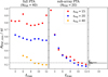 |
Fig. 5 Minimum PSF as function of ℓmax, for different combinations of régularisation cut-offs, sreg. Left: 40 PSRs. Middle: 20 PSRs. Right: distribution of area equivalents, Ann, of the nearest-neighbour distances in the 40-pulsar constellation. |
4.2.3 Determining maximum spherical harmonics degree
The proposed map calculation scheme gives up on the rule of thumb to determine ℓmax, and technically allows one to choose ℓmax deliberately large, as long as we properly regularise the result. In practice this is not recommended, as the dimensions of the matrices involved in the calculation depend on Nmodes, and algebraic operations may become computationally unfeasible. Hence, we need to develop a new approach to determine ℓmax.
We established in the previous section that the maximum local resolution of a PTA is closely linked to the nearestneighbour angular distance distribution in the PTA. Moreover, we show in Fig. 5 that the distribution mean of the areaequivalent, ĀNN, is a conservative tracer of the expected minimum PSF achievable with the pulsar constellation at hand.
Based on these findings, we suggest deriving ℓmax by comparing the mean nearest-neighbour distance from a real PTA dataset, δ̄nn, to the characteristic extent of the spherical harmonics tessellation. This approach is rooted in the following geometric consideration: it is customary to visualise spherical harmonics via their nodal lines, chequering the sphere with parcels in which the spherical harmonic has a positive sign, and those where it has a negative sign. This tessellation of the sphere can be seen as a proxy of the resolution achievable with the respective spherical harmonic degree, ℓ. For the modes m = −l,..., l of a spherical harmonic of degree l, the mode with m = round(l∕2) has the largest number of parcels across the sphere, and the closest distance of nodes. The diagonal extent of such a patch is given as arccos [sin ((ℓ - m + 2)∕(ℓ - m))]. Therefore, matching the diagonal parcel extent to δ̄nn returns a conservative estimate for ℓmax.
In realistic PTA datasets, the number of pulsars effectively contributing the majority of the measured GWB signal is notably smaller than the total number of pulsars, due to different pulsar sensitivities (Speri et al. 2023). To some degree, this is accounted for by using the distribution mean instead of the minimum nearest-neighbour distance. Clearly, proximity of pulsars alone is not guaranteed to produce a meaningful constraint on the smallest-scale modes, and it is reasonable to assume that those modes would be regularised regardless. Still, it is likely that the proposed approach leads to an overestimation of ℓmax. More refined techniques to determine ℓmax could include identifying the effectively contributing pulsars using the methods presented by Speri et al. (2023), or studying the influence of noise on the PTA resolution, as is detailed in Appendix A. But as we provide a conservative estimate of ℓmax, and the number of spherical harmonics modes are not the bottleneck of the anisotropy analysis. We refer these investigations to future studies.
5 Test of the scheme with MPTA simulation
We tested the performance of the adjusted spherical harmonics expansion scheme by applying them to simulations based on the MPTA 4.5-year dataset, similar to those presented in the appendix of Grunthal et al. (2025). The MPTA 4.5-year dataset comprises 83 pulsars located mostly in the southern hemisphere. The PTA constellation is indicated with the white stars in Figs. 8 and 9. Their size reflects the inverse of their RMS; larger pulsars contribute more to the GW S/N. All pulsars were observed every 14-16 days, creating regular ToA series (Miles et al. 2025a).
Analogously to the simulations used in our previous work, Grunthal et al. (2025), we simulated a simplified version of the dataset, including only white noise. For each pulsar we obtained whitened ToAs from the publicly available MPTA 4.5-year ToAs and ephemerides using the TEMPO2 formIdeal plug-in. This way, the simulated dataset has the same observation times, pulsar positions, and pulsar timing model as the real dataset. We then used the libstempo.toasim functions to add white noise fluctuations (EFAC,EQUAD), as well as different GW signals to the whitened ToAs, creating two datasets:
White noise + isotropic GWB. We injected a Hellings-Downs-correlated common red noise signal with a powerlaw PSD into the simulated dataset. The amplitude and spectral index were chosen to match the values reported by Miles et al. (2025b).
White noise + CGW. We injected a single, monochromatic CGW signal into the dataset. In order to test the resolution in the area with a high pulsar desity, we located the supermassive black hole binary at RA 18h DEC -45°. We set fgw = 1 × 10⁻⁸ Hz, so that the source falls between the first and second MPTA frequency bin. To achieve a significantly visible source, without giving up monochromaticity we set Mc = 1 × 10⁸ M⊙ and dL = 1 Mpc.
We analysed both simulations using the regularised spherical harmonics set-up, and obtained narrow-band pulsar pair cross-correlations using DEFIANT (Gersbach et al. 2025). For consistency with the MPTA 4.5-year analyses, we kept sreg = 32, which was determined as the standard choice for the anisotropy analyses of that dataset (Grunthal et al. 2025). In both cases, we set the common red noise parameters in the analysis noise specifications to log10 AGWB = −13.8, γGWB = 3.41. For the reader familiar with the simulations performed in our previous paper (Grunthal et al. 2025), we highlight that the value of log10 AGWB chosen for the anisotropy analysis in this work is slightly larger, leading to smaller S/N and p values in the clean sky maps. This adjustment was necessary in order to keep the S/N range of the CGW recovery for all set-ups in the well-tested range for this analysis method.
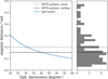 |
Fig. 6 Estimation of the ℓmax based on the spherical harmonics geometry. Left: minimum spherical harmonics tessellation extent at a given degree, ℓ. Right: MPTA nearest-neighbour distance distribution. |
5.1 Determination of ℓmax
Using the method suggested in Section 4.2.3, we find for the MPTA dataset ℓmax = 31. A visualisation of the area-matching process together with the nearest-neighbour distance distribution of the MPTA is shown in Fig. 6. In order to shed light on the change of the result with varying ℓmax, we decided to also analyse the datasets with ℓmax = {16,21}.
A representation of the maximum spherical harmonics tessellation achieved with these ℓmax, in comparison to the underresolving tessellation of ℓmax = 8, is shown in Fig. 7. The sky maps show the spherical harmonic mode with the largest number of knots, as well as the position of the MPTA pulsars as white stars.
5.2 Results
We analysed both simulations with ℓmax = {8,16,21,31} and set sreg = 32 to maintain comparability to the simulation analyses in our previous work (Grunthal et al. 2025). The clean S/N maps of the CGW recovery are shown in Fig. 8. The visibly reduced area and blur of the hotspot demonstrate that increasing ℓmax beyond 8 leads to a better constraint on the source location. With ℓmax = 8, the recovered hotspot has an angular size of 0.25 sr; for ℓmax = 31, the size decreases to 0.15 sr. Simultaneously, the increased maximum of the colour bar indicates a slight increase in the maximum S/N of the hotspot. This shows that the finer spherical harmonics tessellation allows us to exclude additional noise in the relevant spherical harmonics modes, which was broadening the hotspot in the coarser expansion before. In all three cases, the S/N, the corresponding p value, the hotspot area, and the position of the pixel with maximum S /N are collected in Table 1. We also find that overall the localisation of the hotspot improves. With increasing ℓmax, the right ascension of the recovered hottest pixel corresponds significantly better to the CGW position (changed from 18h24m to 18h04m for ℓmax = 31), but it becomes slightly offset in declination (changed from -45° to -46° for ℓmax = 31). We also notice that no artificial hotspots appear at higher ℓmax, which demonstrates the stability of our approach.
Studying the map evolution between ℓmax = 16 and 31, we find the previously explored convergence behaviour towards a minimal local resolution. The maximum S/N and the spatial resolution of the hotspot do not improve significantly. We only find more pronounces traces of the residual diffraction pattern on the northern hemisphere. Looking closer at the extent of the hotspot of the maps in Fig. 8, we find that they behave in the manner described by Boyle & Pen (2012). The resolution of a point source, or similarly the extent of the hotspot, is given by the smallest quadrilateral of pulsars surrounding the source position.
Similarly, we analysed a simulation containing an isotropic GWB injection. The resulting clean S /N maps, displayed in Fig. 9, illustrate that varying the spherical harmonics expansion does not have a significant influence on the maps’ maximum S /N. Additionally, it can be seen by eye that a larger ℓmax makes the recovery look more isotropic in sky areas with a sparse pulsar population. The maximum S /N values and corresponding p values are collected in Table 1 as well. Interestingly, S /Nmax even decreases with larger ℓmax. This is another manifestation of how the more realistic local resolution mitigates signal confusion due to noise being collected across overly large patches. Across all three spherical harmonics expansions, the p values are similar, consistent with an isotropic background. Most importantly, this means that our method does not give rise to artificially large S /N values in the absence of any actual anisotropy.
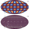 |
Fig. 7 Visual comparison of the spherical harmonics tessellation to the MPTA pulsar constellation. Top: ℓmax = 8. Bottom: ℓmax = 31. |
Characteristic quantities of the MPTA simulations’ anisotropy analyses.
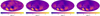 |
Fig. 8 Regularised, clean S/N maps of the first frequency bin (7 nHz) for the simulated MPTA datasets containing WN and a single CGW source at RA 18h DEC −45°. From left to right, the spherical harmonics expansion is set to ℓmax = {8,16,21,31}. For all maps, the regularisation cut-off is set to sreg = 32. |
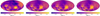 |
Fig. 9 Regularised, clean S/N maps of the first frequency bin (7 nHz) for the simulated MPTA datasets with WN and isotropic GWB injection. From left to right, the regularised spherical harmonics analysis is set up with to ℓmax = {8,16,21,31} and sreg = 32. |
6 Summary and outlook
This work builds on our previous publication (Grunthal et al. 2025) and contains two major results. We develop a framework to evaluate the PSF of a PTA dataset depending on the choice of parameters of the anisotropy analysis. As a second result, we demonstrate with this framework that the regularisa-tion scheme allows us to alter the spherical harmonics expansion of the anisotropy analysis, such that it reflects the local PTA resolution more realistically. We hence present a reworked anisotropy analysis scheme, which can be summarised in two steps:
We determine suitable values for ℓmax (the maximum spherical harmonic degree of the expansion) based on the mean or median of the distribution of pulsars in the PTA;
We remove poorly unconstrained modes by imposing a reg-ularisation threshold, so that the number of modes is comparable to (or smaller than) the number of pulsars: sreg ≤ NPSR. For real PTA datasets, the choice of sreg is also influenced by the quality of the pulsars (Grunthal et al. 2025), such that it is likely smaller than NPSR (for example, sreg was chosen to be 32 for the MPTA 4.5-year analysis, due to the noise and sensitivity properties of the dataset).
We tested this scheme with simulations based on the MPTA 4.5-year PTA dataset. Analysing a continuous-wave injection, we achieved a factor of two improvement in the statistical significance compared to the method from Grunthal et al. (2025). On top of this, we improved the area constraint of the corresponding hotspot by 40% compared to the classical scheme. This demonstrates that in areas with high pulsar densities the better reflected PTA resolution leads to a significantly refined localisability of hotspots.
We recommend that future pulsar timing anisotropy analyses use this updated scheme to set up the analysis parameters. Aside from the improved statistical significance of a potential anisotropy, optimised PTA sky maps connect naturally to targeted searches for individual supermassive black hole binaries, as they facilitate follow-up studies.
The current bottleneck of the analysis is the calculation of the pulsar-pair cross correlations, so as PTAs grow, an efficient implementation of this step is key to a fast anisotropy analysis. Forthcoming studies can also focus on fine-tuning the scheme for estimating ℓmax, as is detailed in Sect. 4.2.3.
Furthermore, there are a number of applications of the PSF framework beyond the scope of this paper. Future work may target the impact of noise misspecification on angular resolution, the interplay between residual noise and the regularisation scheme, and the sky position recovery of point sources. It may also be interesting to investigate whether it is possible to optimise PTA set-ups such that the corresponding sky maps target regions of high interest; for example, the Virgo cluster or around continuous-wave candidates.
Data availability
The code developed and used for this work can be accessed under https://github.com/mpta-gw/cartography.git.
Acknowledgements
KG, DC and MK acknowledge continuing valuable support from the Max-Planck society. KG acknowledges support from the International Max Planck Research School (IMPRS) for Astronomy and Astrophysics at the Universities of Bonn and Cologne. ET and RSN acknowledge support from the Australian Research Council (ARC) Centres of Excellence CE170100004 and CE230100016 and ARC DP230103088. MK acknowlegdes support by the CAS-MPG legacy Programme. MM acknowledges support from the NANOGrav Collaboration’s National Science Foundation (NSF) Physics Frontiers Center award numbers 1430284 and 2020265. This publication made use of open source python libraries including numpy (Harris et al. 2020), scipy (Virtanen et al. 2020), matplotlib (Hunter 2007), and healpy (Górski et al. 2005), as well as the python-based pulsar analysis packages, libstempo, enterprise (Ellis et al. 2020), ENTERPRISE_EXTENSIONS (Taylor et al. 2021) and DEFIANT (Gersbach et al. 2025).
References
- Abadie, J., Abbott, B. P., Abbott, R., et al. 2011, Phys. Rev. Lett., 107, 271102 [Google Scholar]
- Agarwal, N., Agazie, G., Anumarlapudi, A., et al. 2026, ApJ, 998, L11 [Google Scholar]
- Agazie, G., Alam, M. F., Anumarlapudi, A., et al. 2023a, ApJ, 951, L9 [CrossRef] [Google Scholar]
- Agazie, G., Anumarlapudi, A., Archibald, A. M., et al. 2023b, ApJ Lett., 956, L3 [Google Scholar]
- Ali-Haïmoud, Y., Smith, T. L., & Mingarelli, C. M. F. 2021, Phys. Rev. D, 103, 042009 [Google Scholar]
- Allen, B., & Ottewill, A. C. 1997, Phys. Rev. D, 56, 545 [Google Scholar]
- Allen, B., & Romano, J. D. 1999, Phys. Rev. D, 59, 102001 [NASA ADS] [CrossRef] [Google Scholar]
- Allen, B., & Romano, J. D. 2023, Phys. Rev. D, 108, 043026 [NASA ADS] [CrossRef] [Google Scholar]
- Banagiri, S., Criswell, A., Kuan, T., et al. 2021, MNRAS, 507, 5451 [Google Scholar]
- Begelman, M. C., Blandford, R. D., & Rees, M. J. 1980, Nature, 287, 307 [Google Scholar]
- Boyle, L., & Pen, U.-L. 2012, Phys. Rev. D, 86, 124028 [Google Scholar]
- Burke-Spolaor, S., Taylor, S. R., Charisi, M., et al. 2019, A&A Rev., 27, 5 [NASA ADS] [CrossRef] [Google Scholar]
- Caprini, C., Chala, M., Dorsch, G. C., et al. 2020, J. Cosmology Astropart. Phys., 2020, 024 [Google Scholar]
- Chamberlin, S. J., Creighton, J. D. E., Siemens, X., et al. 2015, Phys. Rev. D, 91, 044048 [NASA ADS] [CrossRef] [Google Scholar]
- Cornish, N. J. 2001, CQG, 18, 4277 [Google Scholar]
- Cornish, N. J., & van Haasteren, R. 2014, arXiv e-prints [arXiv:1406.4511] [Google Scholar]
- Demorest, P. B., Ferdman, R. D., Gonzalez, M. E., et al. 2013, ApJ, 762, 94 [Google Scholar]
- Detweiler, S. 1979, ApJ, 234, 1100 [NASA ADS] [CrossRef] [Google Scholar]
- Domènech, G. 2021, Universe, 7, 398 [Google Scholar]
- D’Orazio, D. J., & Charisi, M. 2023, Black Holes in the Era of Gravitational Wave Astronomy (Elsevier), Ch. 5 [Google Scholar]
- Ellis, J. A., Vallisneri, M., Taylor, S. R., & Baker, P. T. 2020, https://doi.org/10.5281/zenodo.4059815 [Google Scholar]
- EPTA Collaboration and InPTA Collaboration (Antoniadis, J., et al.) 2023, A&A, 678, A50 [CrossRef] [EDP Sciences] [Google Scholar]
- Floden, E., Mandic, V., Matas, A., & Tsukada, L. 2022, Phys. Rev. D, 106, 023010 [Google Scholar]
- Gair, J., Romano, J. D., Taylor, S., & Mingarelli, C. M. F. 2014, Phys. Rev. D, 90, 082001 [NASA ADS] [CrossRef] [Google Scholar]
- Gersbach, K. A., Taylor, S. R., Meyers, P. M., & Romano, J. D. 2025, Phys. Rev. D, 111, 023027 [Google Scholar]
- Górski, K. M., Hivon, E., Banday, A. J., et al. 2005, ApJ, 622, 759 [Google Scholar]
- Grunthal, K., Nathan, R. S., Thrane, E., et al. 2025, MNRAS, 536, 1501 [Google Scholar]
- Gualandris, A., Read, J. I., Dehnen, W., & Bortolas, E. 2017, MNRAS, 464, 2301 [Google Scholar]
- Guzzetti, M. C., Bartolo, N., Liguori, M., & Matarrese, S. 2016, Nuovo Cimento Riv. Ser., 39, 399 [Google Scholar]
- Harris, C. R., Millman, K. J., van der Walt, S. J., et al. 2020, Nature, 585, 357 [NASA ADS] [CrossRef] [Google Scholar]
- Hellings, R. W., & Downs, G. S. 1983, ApJ, 265, L39 [NASA ADS] [CrossRef] [Google Scholar]
- Hindmarsh, M. B., & Kibble, T. W. B. 1995, Rep. Progr. Phys., 58, 477 [Google Scholar]
- Hindmarsh, M., Lüben, M., Lumma, J., & Pauly, M. 2021, SciPost Phys. Lect. Notes, 024 [Google Scholar]
- Holley-Bockelmann, K., & Khan, F. M. 2015, ApJ, 810, 139 [Google Scholar]
- Hunter, J. D. 2007, Comput. Sci. Eng., 9, 90 [NASA ADS] [CrossRef] [Google Scholar]
- Kormendy, J., & Richstone, D. 1995, ARA&A, 33, 581 [Google Scholar]
- Kudoh, H., & Taruya, A. 2005, Phys. Rev. D, 71, 024025 [Google Scholar]
- Lasky, P. D., Mingarelli, C. M. F., Smith, T. L., et al. 2016, Phys. Rev. X, 6, 011035 [NASA ADS] [Google Scholar]
- Maggiore, M. 2000, Phys. Rept., 331, 283 [CrossRef] [Google Scholar]
- Miles, M. T., Shannon, R. M., Reardon, D. J., et al. 2025a, MNRAS, 536, 1467 [Google Scholar]
- Miles, M. T., Shannon, R. M., Reardon, D. J., et al. 2025b, MNRAS, 536, 1489 [Google Scholar]
- Milosavljevic, M., & Merritt, D. 2003, AIP Conf. Proc., 686, 201 [NASA ADS] [CrossRef] [Google Scholar]
- Mingarelli, C. M. F., Sidery, T., Mandel, I., & Vecchio, A. 2013, Phys. Rev. D, 88 [Google Scholar]
- Mingarelli, C. M. F., Lazio, T. J. W., Sesana, A., et al. 2017, Nat. Astron., 1, 886 [Google Scholar]
- Mitra, S., et al. 2008, Phys. Rev. D, 77, 042002 [Google Scholar]
- Pol, N., Taylor, S. R., & Romano, J. D. 2022, ApJ, 940, 173 [NASA ADS] [CrossRef] [Google Scholar]
- Rajagopal, M., & Romani, R. W. 1995, ApJ, 446, 543 [NASA ADS] [CrossRef] [Google Scholar]
- Reardon, D. J., Zic, A., Shannon, R. M., et al. 2023, ApJ Lett., 951, L6 [Google Scholar]
- Romano, J. D., & Cornish, N. J. 2017, Liv. Rev. Relativ., 20, 2 [Google Scholar]
- Romano, J. D., & Allen, B. 2024, CQG, 41, 175008 [Google Scholar]
- Rosado, P. A., Sesana, A., & Gair, J. 2015, MNRAS, 451, 2417 [NASA ADS] [CrossRef] [Google Scholar]
- Ryu, T., et al. 2018, MNRAS, 473 [Google Scholar]
- Saikawa, K. 2017, Universe, 3, 40 [Google Scholar]
- Sazhin, M. V. 1978, Soviet Ast., 22, 36 [NASA ADS] [Google Scholar]
- Sesana, A., & Vecchio, A. 2010, CQG, 27, 084016 [Google Scholar]
- Sesana, A., Haardt, F., Madau, P., & Volonteri, M. 2004, ApJ, 611, 623 [NASA ADS] [CrossRef] [Google Scholar]
- Speri, L., Porayko, N. K., Falxa, M., et al. 2023, MNRAS, 518, 1802 [Google Scholar]
- Taylor, S. R., & Gair, J. R. 2013, Phys. Rev. D, 88, 084001 [NASA ADS] [CrossRef] [Google Scholar]
- Taylor, S. R., Mingarelli, C. M. F., Gair, J. R., et al. 2015, Phys. Rev. Lett., 115, 041101 [NASA ADS] [CrossRef] [Google Scholar]
- Taylor, S. R., van Haasteren, R., & Sesana, A. 2020, Phys. Rev. D, 102, 084039 [NASA ADS] [CrossRef] [Google Scholar]
- Taylor, S. R., Baker, P. T., Hazboun, J. S., Simon, J., & Vigeland, S. J. 2021, https://github.com/nanograv/enterprise_extensions [Google Scholar]
- Thrane, E., Ballmer, S., Romano, J. D., et al. 2009, Phys. Rev. D, 122002 [Google Scholar]
- Virtanen, P., Gommers, R., Oliphant, T. E., et al. 2020, Nat. Methods, 17, 261 [Google Scholar]
- Xu, H., Chen, S., Guo, Y., et al. 2023, RAA, 23, 075024 [NASA ADS] [Google Scholar]
- Yardley, D. R. B., Hobbs, G. B., Jenet, F. A., et al. 2010, MNRAS, 407, 669 [NASA ADS] [CrossRef] [Google Scholar]
- Yuan, C., & Huang, Q.-G. 2021, iScience, 24, 102860 [Google Scholar]
This approach is mathematically equivalent to the calculations in Grunthal et al. (2025), but the code is simpler and streamlined with standard PTA GW searches thanks to the narrow-band optimal statistic. We verified consistency with the Grunthal et al. (2025) results by comparing the numerical values of all matrices used during the sky map calculation.
φ̃(fk) has the shape (2kmax × 2kmax) and two adjacent non-zero components, because the Fourier transform matrices contains both a sine and a cosine component for each frequency.
This means that for a spherical harmonics expansion to ℓmax, where we have (ℓmax + 1)2 modes, sreg ≤; (ℓmax + 1)2.
As is explained in more detail in Grunthal et al. (2025), P′k and  can have negative values, due to residual noise present in the data.
For N points on the sphere, their positions are given by θi = (2πi)/φ and ϕ = arccos(1 − 2i/N), with the golden ratio φ = (1 + √5)/2.
In reality, this area is rather a polygonal structure on a spherical surface. Hence, the approximation may slightly overestimate the actual area marked out by the nearest pulsars, but it is sufficient to compare the achievable resolution to the expected diffraction limit.
Appendix A Extension of the point spread formalism to evaluate noise misspecification
Despite growing efforts to model the noise budget of the pulsars in a PTA dataset as accurately as possible, all PTA data analysis is prone to noise misspecification, i.e. an unmodelled noise budget left in the data. For example, comparing the noise models used in the EPTA DR2 GWB analysis (EPTA Collaboration and InPTA Collaboration 2023) to those employed in the MPTA 4.5-year GW analysis (Miles et al. 2025a), we find an increasing variety of noise processes found in datasets, mainly owing to an improved ToA precision and higher observing frequency bandwidths. This raises the question, if these noise contributions have been present in the EPTA dataset yet remained unnoticed. After all, there is currently no way to absolutely determine the precise and accurate noise model of every pulsar.
It is safe to assume that residual noise also affects the sensitivity of a PTA to potential GWB anisotropies. We can expect it to contribute to the blurring of a single source during the recovery, increasing the size of the PSF. Hence it is desirable to ultimately include this effect in the PSF calculation framework developed in Sect. 3.
In the frequentist anisotropy analysis, the noise budget enters the clean map calculation via the Fisher matrix M, as it contains the cross-correlation covariance matrix Σ, whose entries are determined from the noise parameters (e.g. the white noise parameters EFAC, EQUAD, the red noise spectral parameters A and γ, etc.).
We can generalise the PTA PSF calculation scheme to allow for a hypothetical noise misspecification by altering the Fisher matrices entering Eq. (26). The Fisher matrix used to construct the dirty map of the hot pixel, now denoted by M, contains the ‘true’ noise values in its true cross-correlation covariance matrix, S. The (regularised) inverted Fisher matrix, M-1, is calculated with different noise values, representing the noise misspecification. The clean map recovered for a single hot pixel is now given as:
 (A.1)
(A.1)
While Eq. (A.1) now fully depicts a realistic recovery process, it is desirable to single out the individual contributions of both the regularisation procedure and a potential noise misspecification to the broadening of the hot pixel in the recovered clean map,  . To this end we rearrange M̃-1M in Eq. (A.1), as
 (A.2)
(A.2)
 (A.3)
(A.3)
 (A.4)
(A.4)
factorising it into the regularisation contribution (cf. Eq.(29)) and the noise misspecification contribution, which we defined as  .
.
Using the definition of the Fisher matrix, M ≡ R†Σ−1R, we find an alternative expression for the noise misspecification contribution,
 (A.5)
(A.5)
 (A.6)
(A.6)
emphasising the role of the pulsar-pair cross covariance matrix in the noise model contribution to the PTA PSF.
Putting together Eqs. (A.1) and (A.4), the general expression for the PSF calculation now reads:
 (A.7)
(A.7)
This factorisation demonstrates a couple of noteworthy points: Even without applying a regularisation scheme (Λsreg = 1), a point source is blurred due to residual noise in the dataset. More broadly speaking, any deviation of both Λs and N from a unit matrix gives rise to a PSF. Furthermore we observe that we can consistently recover Eq. (A.1) assuming perfect noise models, i.e. N = 1, as indicated in Sec. 3.2. Finally we note that — being read from right to left according to the matrix multiplication — Eq. (A.7) is satisfyingly a mathematical reflection the loss of information throughout the anisotropy analysis: First due to noise misspecification, then due to the regularisation.
All Tables
All Figures
|
Fig. 1 Single hot pixel seen through a 40PSR PTA with different regularisation cut-offs. The crosshair indicates the position of the hot pixel. Top: clean map with ℓmax = 8, sreg = 15. Bottom: clean map with ℓmax = 8, Sreg = 40. |
| In the text | |
|
Fig. 2 Sky maps showing the (S/N-based) PSF of the PTA as a function of sky position. The white stars indicate the positions of the pulsars in the respective PTA. Both plots were calculated using the classic spherical harmonics expansion scheme based on the number of pulsars. Top: 40 pulsar PTA, ℓmax = 5, sreg = 35. Bottom: 20 pulsar subset PTA, ℓmax = 3, sreg = 15. |
| In the text | |
|
Fig. 3 Point spread area sky maps for the 40 pulsar isotropic PTA set-up. From left to right: ℓmax = {6,8,10,12}. The white stars indicate the pulsar positions. |
| In the text | |
|
Fig. 4 Point spread area sky maps for the 20-pulsar sub-array of the 40 pulsar isotropic PTA set-up. From left to right: ℓmax = {4,8,10,12}. The white stars indicate the pulsar positions. |
| In the text | |
|
Fig. 5 Minimum PSF as function of ℓmax, for different combinations of régularisation cut-offs, sreg. Left: 40 PSRs. Middle: 20 PSRs. Right: distribution of area equivalents, Ann, of the nearest-neighbour distances in the 40-pulsar constellation. |
| In the text | |
|
Fig. 6 Estimation of the ℓmax based on the spherical harmonics geometry. Left: minimum spherical harmonics tessellation extent at a given degree, ℓ. Right: MPTA nearest-neighbour distance distribution. |
| In the text | |
|
Fig. 7 Visual comparison of the spherical harmonics tessellation to the MPTA pulsar constellation. Top: ℓmax = 8. Bottom: ℓmax = 31. |
| In the text | |
|
Fig. 8 Regularised, clean S/N maps of the first frequency bin (7 nHz) for the simulated MPTA datasets containing WN and a single CGW source at RA 18h DEC −45°. From left to right, the spherical harmonics expansion is set to ℓmax = {8,16,21,31}. For all maps, the regularisation cut-off is set to sreg = 32. |
| In the text | |
|
Fig. 9 Regularised, clean S/N maps of the first frequency bin (7 nHz) for the simulated MPTA datasets with WN and isotropic GWB injection. From left to right, the regularised spherical harmonics analysis is set up with to ℓmax = {8,16,21,31} and sreg = 32. |
| In the text | |
Current usage metrics show cumulative count of Article Views (full-text article views including HTML views, PDF and ePub downloads, according to the available data) and Abstracts Views on Vision4Press platform.
Data correspond to usage on the plateform after 2015. The current usage metrics is available 48-96 hours after online publication and is updated daily on week days.
Initial download of the metrics may take a while.