| Issue |
A&A
Volume 706, February 2026
|
|
|---|---|---|
| Article Number | A4 | |
| Number of page(s) | 14 | |
| Section | Planets, planetary systems, and small bodies | |
| DOI | https://doi.org/10.1051/0004-6361/202557986 | |
| Published online | 28 January 2026 | |
Resolving the terrestrial planet-forming region of HD 172555 with ALMA
I. Post-impact dust distribution
1
School of Physics, Trinity College Dublin, the University of Dublin, College Green,
Dublin 2,
Ireland
2
Malaghan Institute of Medical Research, Gate 7, Victoria University,
Kelburn Parade,
Wellington
6012,
New Zealand
3
School of Physics and Astronomy, University of Exeter, Astrophysics Group,
Stocker Road,
Exeter
EX4 4QL,
UK
4
Space Science Institute,
4750 Walnut Street, Suite 205,
Boulder,
CO
80301,
USA
5
Steward Observatory, University of Arizona,
933 N. Cherry Avenue,
Tucson,
AZ
85721-0065,
USA
6
Center for Astrophysics, Harvard & Smithsonian,
60 Garden Street,
Cambridge,
MA
02138,
USA
7
Institute of Astronomy, University of Cambridge,
Madingley Road,
Cambridge CB3 OHA,
UK
8
Department of Physics, Astronomy, & Geosciences, Towson University,
8000 York Road,
Towson,
MD
21252,
USA
★ Corresponding author: This email address is being protected from spambots. You need JavaScript enabled to view it.
Received:
5
November
2025
Accepted:
2
December
2025
Abstract
Context. Giant impacts between planetary embryos are a natural step in the terrestrial planet formation process and are expected to create disks of warm debris in the terrestrial regions of their stars. Understanding the gas and dust debris produced in giant impacts is vital for comprehending and constraining models of planetary collisions.
Aims. We reveal the distribution of millimeter (mm) grains in the giant impact debris disk of HD 172555 for the first time, using new ALMA 0.87 mm observations at ∼80 mas (2.3 au) resolution.
Methods. We modeled the interferometric visibilities to obtain basic spatial properties of the disk and compared these data to the disk’s dust and gas distributions at other wavelengths.
Results. We detected the star and dust emission from an inclined disk out to ∼9 au and down to 2.3 au (on-sky) from the central star, with no significant asymmetry in the dust distribution. The radiative transfer modeling of the visibilities indicates the disk surface density distribution of mm grains most likely peaks around ∼5 au, while the width inferred remains model-dependent at the S/N of the data. We highlighted an outward radial offset of the small grains traced by scattered light observations compared to the mm grains, which could be explained by the combined effect of gas drag and radiation pressure in the presence of large enough gas densities. Furthermore, our SED modeling implies a size distribution slope for the mm grains consistent with the expectation of collisional evolution and flatter than inferred for the micron-sized grains, implying a break in the grain size distribution and confirming an overabundance of small grains.
Key words: techniques: interferometric / planets and satellites: formation / stars: individual: HD 172555 / submillimeter: planetary systems
© The Authors 2026
 Open Access article, published by EDP Sciences, under the terms of the Creative Commons Attribution License (https://creativecommons.org/licenses/by/4.0), which permits unrestricted use, distribution, and reproduction in any medium, provided the original work is properly cited.
This article is published in open access under the Subscribe to Open model. This email address is being protected from spambots. You need JavaScript enabled to view it. to support open access publication.
1 Introduction
Even after the gas-rich protoplanetary disk phase of planetary formation ends, terrestrial planet formation continues in the inner regions of planetary systems during the era of giant impacts. This phase, between ∼10 and 100 Myr, is dominated by the growth of planetary embryos through mutual collisions, eventually achieving final planet masses and orbital configurations (e.g., Chambers 2001; Morbidelli et al. 2012, and references therein). There is plenty of evidence that an era of impacts took place in the Solar System, as evidenced, for example, by the formation of our own Moon (e.g., Cameron & Ward 1976; Canup & Asphaug 2001; Canup 2004), Mercury’s iron enrichment (e.g., Benz et al. 1988; Cameron et al. 1988; Benz et al. 2007), and the Martian hemispheric dichotomy (e.g., Wilhelms & Squyres 1984; Smith et al. 1999; Andrews-Hanna et al. 2008). Outside the Solar System, indirect evidence is found in exoplanet populations – for example, in the statistics of mature close-in super-Earth planetary systems (Izidoro & Raymond 2018, and references therein) – and in the presence of warm dust in the inner few au regions of ∼3% of 10–100 Myr-old stars (Kennedy & Wyatt 2013).
In general, it is difficult to distinguish between steady-state phenomena (asteroid belt analogs, e.g., Su et al. 2013) and non-steady-state phenomena (giant impacts or other transient events, e.g., Geiler & Krivov 2017) as the origin of the warm dust in the inner regions (a few au) of these stars. In an effort to distinguish between disks created by steady-state and non-steady-state phenomena, Wyatt et al. (2007) created an analytical model for the steady-state collisional evolution of disks, which shows that at a given radial location and system age, there is a maximum possible fractional infrared (IR) luminosity a disk can have due to collisional processing. Disks with an IR luminosity below this maximum can be explained by steady-state phenomena, such as asteroid belts, but disks with infrared luminosities above the maximum allowed value cannot be produced in this way and instead must be undergoing a transient event, such as a giant impact (Wyatt et al. 2007). In a few of these extremely high fractional luminosity systems, mid-IR (MIR) spectroscopy additionally shows a unique dust mineralogy with features from glassy silica, a thermodynamically altered mineral that requires high temperature processing and vapor condensation, naturally provided by a hypervelocity, planetary-scale impact (e.g., Lisse et al. 2009; Johnson et al. 2012). Of the known young, warm, and extremely dusty debris disks, only three systems in the expected age of terrestrial planet formation show this glassy silica feature in their Spitzer spectra: HD 23514 (Rhee et al. 2008; Meng et al. 2012), HD 15407A (Fujiwara et al. 2012; Olofsson et al. 2012), and the focus of this paper, HD 172555 (Chen et al. 2006; Lisse et al. 2009). Recent James Webb Space Telescope (JWST) MIR spectra further reveal a handful of newly identified extremely dusty debris disks that are rich in silica dust (Su et al., in prep.).
With multiple lines of evidence pointing to a giant impact scenario as the origin of the debris, HD 172555 (HR 7012, HIP 92024) is one of the best characterized systems with warm dust. HD 172555 is an A7V (Gray et al. 2006) star at a distance of 28.79±0.13 pc from Earth (Gaia Collaboration 2022) and is a member of the β Pictoris moving group (Zuckerman et al. 2001). The age of the moving group has been estimated to be 23.4±4.8 Myr (Olivares et al. 2025). HD 172555 hosts a close to edge-on debris disk, with an inclination of 76.2◦±1.7◦, reported by Engler et al. (2018) as 103.8◦±1.7◦. The system’s IR fractional luminosity is 7.2 × 10⁻⁴ (Mittal et al. 2015), which is ∼300 times larger than the maximum allowed IR luminosity given by the age and disk radius of HD 172555 (Wyatt et al. 2007). SED fitting of the system shows the IR excess is best fit by warm, ∼290 K dust (Cote 1987), and fitting of the MIR Spitzer continuum and solid-state features requires a non-steady-state particle size distribution, with an overabundance of small grains (Lisse et al. 2009; Johnson et al. 2012). The latter also supports the impact scenario, as the overabundance of small grains indicates that the circumstellar material must have been created relatively recently and in a transient event.
The final piece of evidence for the impact scenario comes from the Atacama Large Millimeter/submillimeter Array (ALMA) detection of 12CO J=2–1 emission at 1.3 mm (Schneiderman et al. 2021). These Cycle 1 observations detect both the continuum and 12CO, which are both spatially unresolved, with a resolution of 1.16″ × 0.75″ (33.4×21.6 au). However, using the fact that the 12CO is spectrally resolved, Schneiderman et al. (2021) constrain the CO to a ring of radius ∼7.5 au. At this location around an A star, asteroids would be too warm to retain CO or CO2 ice for subsequent release over the age of the system (e.g., Prialnik & Rosenberg 2009; Snodgrass et al. 2017, and references therein). Schneiderman et al. (2021) explore four scenarios for the origin of both the dust and CO in the system: leftover from a primordial protoplanetary disk, collisional production in an asteroid belt, inward transport from an outer reservoir, and release in the aftermath of a giant impact. They favor the giant impact between planetary-sized bodies with atmospheric stripping scenario as it is the only one that can explain the dust mineralogy, particle size distribution, dust mass, radial distribution of dust and CO, and total amount of CO detected. However, because these observations were spatially unresolved, the spatial distribution of the millimeter (mm) grains remains unknown.
Observations of HD 172555 at other wavelengths reveal the presence of smaller dust grains and atomic gas in the system. In the MIR, using multiepoch photometry and spectroscopy, no evidence was found for variability in the HD 172555 system (Su et al. 2020). Combined with later JWST observations, this indicates that the submicron grains produced in the impact are stable on decades-long timescales (Su et al. 2020; Samland et al. 2025). HD 172555 has been spatially resolved in the MIR using interferometry and imaging (Smith et al. 2012) and in the optical using scattered light imaging (Engler et al. 2018); both of these observations constrain the outer edge of the dust emission to 8– 10 au and present marginal evidence for an asymmetry in the dust distribution. Overall, the small grains probed by the MIR and scattered light observations appear to be roughly co-located with the CO detected by ALMA (Schneiderman et al. 2021), suggesting that the impact took place in this region.
The innermost region of the HD 172555 planetary system (a few stellar radii to <0.5 au) shows signs of inward transport of material and dynamic upheaval. Star-grazing bodies (exocomets) have been detected transiting at ∼7 stellar radii from the central star through time-variable absorption in the Ca II K and H doublet lines in the UV and in the optical light curve (Kiefer et al. 2014, 2023). This provides further evidence for the planetary system being close to edge-on. Kiefer et al. (2023) calculated the evaporation efficiency for both the exocomet transit they found in the optical light curve and the exocomets detected spectroscopically by Kiefer et al. (2014) and concluded there are likely at least two classes of exocomets in this system. Some of the gas emission in this system has been attributed to these exocomets. Using the Hubble Space Telescope, Grady et al. (2018) detected Si III, Si IV, C II, C IV, and O I absorption from exocomets originating from the warm dust disk and potentially perturbed onto star-grazing orbits by a Jovian-mass planet. Cl I, S I, Ni II, and Fe II emission from a gaseous disk <0.5 au from the star, believed to be from evaporating rocky bodies, was detected with JWST (Samland et al. 2025). This hot gas is likely to have been predominantly released in situ and could be linked to the giant impact, as the impact could have led to increased dynamical activity in the system which led to increased collisional interactions or the production of dust that can drift inward and sublimate (Samland et al. 2025, and references therein). Finally, spectrally and spatially unresolved O I emission from a circumstellar disk was detected with the Herschel Space Observatory, which could have been released in the giant impact or accumulated slowly over time from collisions within a belt of dust (Riviere-Marichalar et al. 2012). The O I emission could have originated in the giant impact, as silicate constituents (Si, Fe, Mg, and O) can be produced in gas form during a hypervelocity impact (Pahlevan et al. 2011) or from the photodissociation of volatile molecules originating in the stripped atmosphere (Schneiderman et al. 2021). However, we do not presently know whether the O I is co-located with the CO or with the hot atomic gas revealed by JWST.
To better constrain the radial and azimuthal distribution of the impact-produced dust at a few au around HD 172555, we present follow-up high-resolution 0.87 mm continuum observations with ALMA. In Sect. 2, we describe our observations, calibration, and imaging. In Sect. 3, we present the first resolved image of dust around HD 172555 at mm wavelengths. Section 4 describes the modeling we performed on the data visibilities to determine basic disk parameters. In Sect. 5, we discuss our findings in the context of the literature and we conclude with a summary in Sect. 6.
2 Observations
We observed the HD 172555 system for a total of 6.6 hours on-source with ALMA on Chajnantor, Chile during Cycle 9 through project 2022.1.00793.S (PI: Matrà). Observations were split between a lower and higher spectral setup covering different frequencies within Band 7 (0.87 mm). All the observations were carried out using Band 7 receivers and the 12-meter array, with baselines ranging between 27.5 and 3637.7 m for each setup. Observations in the lower spectral setup were taken on five separate days between 16 May and 3 June 2023, while observations in the higher spectral setup were taken at four times between 3 and 4 June 2023.
In each of the higher and lower spectral setups, four unique spectral windows were used. In the higher setup, all four of the spectral windows were 1.875 GHz wide, centered at 343.2, 345.2, 355.2, and 357.2 GHz, with a channel width of 488.281 kHz. In the lower setup, three of the spectral windows were 1.875 GHz wide, centered at 328.9, 330.9, and 340.9 GHz, and one spectral window was 2 GHz wide centered at 342.9 GHz, with a resolution of 31.3 MHz. The windows in the higher spectral setup were set to cover the CS J=7–6, 12CO J=3–2, HCN J= 4–3, and HCO+ J=4–3 transitions at 342.883, 345.796, 354.505, and 356.734 GHz, respectively. The windows of the lower spectral setup were set to cover the C18O J=3–2, 13CO J=3–2, and CN J=3–2 transitions at 329.331, 330.588, and 340.248 GHz, respectively, as well as the continuum.
Standard calibrations were applied to each visibility dataset by the ALMA observatory using its pipeline. Data manipulation was carried out using the Common Astronomy Software Applications (CASA) software version 6.6.5 (The CASA Team 2022). For the continuum analysis, for each of the four spectral windows in the two spectral setups, we flagged the spectral lines, then time and frequency averaged the visibilities (to 30 seconds and 1.875 GHz, the size of the entire spectral window, respectively) to facilitate the processing of the large dataset while avoiding time- or frequency-smearing effects. We then concatenated all datasets for each spectral window to obtain a final calibrated and time- and frequency-averaged continuum visibility dataset for each spectral setup. We did not implement any astrometric realignment for each observation, as the proper motion and parallax of the system cause motions of at most <12 mas over the maximum time difference between observations, which are about an order of magnitude smaller than the beam and comparable to to the absolute astrometric accuracy1 of our continuum data, ∼13 mas.
We jointly imaged the higher and lower spectral setups in CASA using the CLEAN algorithm (Högbom 1974) implemented through the tclean task. We carried out the continuum imaging in multifrequency synthesis mode with Hogbom deconvolution (Högbom 1974). We chose a natural weighting scheme with a u-v taper of 0.08″ to achieve maximum surface brightness sensitivity (S/N beam−1), while still maintaining some spatial resolution, which led to a beam of 166 × 148 mas (4.8 × 4.3 au at the distance of HD 172555) and a root-mean-square (RMS) noise level of 10.4 µJy beam−1. At the same time, we also created an image using Briggs weighting (Briggs 1995) with a standard robust value of 0.5, obtaining a resolution of 84 × 73 mas (2.4 × 2.1 au) with an RMS noise level of 11.3 µJy beam−1. The primary focus of this work is the analysis of the dust continuum emission. An in-depth analysis of the spectral lines deferred to a future companion paper covering their detection, kinematics, and compositional investigation.
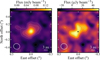 |
Fig. 1 Left: ALMA 0.87 mm continuum emission from the HD 172555 planetary system (star and disk) obtained by joint imaging of the combined visibility dataset. Right: same as the left panel, but imaged after removing the star from the visibilities, as described in Sect. 3. The symbol in the center notes the position of the star. In both panels, north is up and east is left. Contours are ±[2, 4, 6] × 10.4 µJy beam−1, the RMS noise level. Images are made with a natural weighting and a u-v taper, as described in Sect. 2. |
3 Results
The left panel in Fig. 1 shows the final continuum (tapered) image with the combined thermal emission from the central star and the disk in the HD 172555 system. To better constrain the morphology of the circumstellar dust without contamination from the central star, we sought to create a disk-only continuum image using a procedure similar to Matrà et al. (2020). To do so, we assumed the star is a point source and appears with constant amplitude on long baselines. We then iteratively imaged the long-baseline visibilities with a minimum u-v distance cutoff, which we increased at every iteration. We visually identified the minimum u-v distance that allows us to remove the extended disk emission, while still detecting the compact, unresolved central star. We found the best compromise to be a minimum u-v distance of 600 kλ for the lower spectral setup and 700 kλ for the higher spectral setup.
Separately for each spectral setup, assuming the star is an unresolved point source, we fit the visibilities of the longest baselines with the above u-v cutoffs, now unbiased by any disk emission, to obtain a best-fit stellar flux and the right ascension and declination (RA and Dec) position. The results of our stellar fits for each spectral setup are detailed in Table 1. We note that the fluxes are consistent within the errors, which include both random noise and flux calibration uncertainty. We then subtracted the best-fit model visibilities for each spectral setup from the entire visibility dataset for that setup, including all baselines, effectively subtracting the star from our data. Finally, we imaged the star-subtracted visibilities, combining both spectral setups, to obtain a disk-only continuum image, shown in the right panel of Fig. 1.
As seen in both panels of Fig. 1, extended emission from a close to edge-on dust disk is clearly detected along a position angle of ∼120◦, extending out to ∼0.3″, which corresponds to ∼8.6 au from the central star at the distance of HD 172555. The emission appears broad, extending down to the inner resolution element of our observations. Even after accounting for the disk inclination, this indicates dust is emitting down to 2.3 au on-sky from the central star. The orientation and outer radius of the disk are qualitatively consistent with previous scattered light and MIR imaging (Smith et al. 2012; Engler et al. 2018), although our observations are tracing larger mm grains, as opposed to the smaller grains traced by the scattered light and MIR observations. Our ALMA observations reveal the inner <5 au region free from contamination from the central star, as well as spatially resolve the disk continuum in the mm, for the first time.
To compare the results of our observations to what would be expected given the flux density measured by Schneiderman et al. (2021) and the spectral slope of this system in the mm, we measured the flux density of the disk from our disk-only images. Using the CASA task imview and visually defining a region around the disk, we measured the flux density from images created separately from the visibilities from each spectral setup, as well as from imaging of both spectral setups together, as seen in Fig. 1. For the lower (λc = 0.89 mm) and higher (λc = 0.86 mm) spectral setups, we find Fν = 0.26 ± 0.04 mJy and Fν = 0.17 ± 0.03 mJy, respectively, and when we imaged the two spectral setups together, as seen in the right panel of Fig. 1, we measure Fν = 0.18 ± 0.02 mJy, where all quoted errors are 1σ. After accounting for the expected stellar contribution, Schneiderman et al. (2021) report Fν = 0.09 ± 0.03 mJy. Given the observed emission at 1.3 mm by Schneiderman et al. (2021) and the best-fit mm spectral slope (see Sect. 4.4), the emission we observed is consistent with the expected emission within 2σ.
Results from fitting the stellar flux and position.
4 Modeling
4.1 The physical model
To formally constrain the radial structure and geometry of dust, we fit our visibilities using two models, each with two components: an axisymmetric dust disk and the star modeled as a point source. In our first model (hereafter Gaussian model), the radial surface mass density of the disk, Σ, was modeled as a Gaussian, used to determine a centroid radius, R, and full width at half maximum (FWHM, hereafter width), ∆R. For simplicity, we modeled the vertical density distribution of the disk as a Gaussian with the aspect ratio,  , radially fixed to 0.05, as the disk is not vertically resolved. The full dust density distribution in the disk is thus represented as
 (1)
where Σscale is a normalization factor that is proportional to the disk flux, where we fit for the latter (see Sect. 4.2), r and z are the cylindrical coordinates, R and σr are the center and standard deviation of the radial Gaussian disk, respectively, and σz = H = hr. σr and ∆R are related through
(1)
where Σscale is a normalization factor that is proportional to the disk flux, where we fit for the latter (see Sect. 4.2), r and z are the cylindrical coordinates, R and σr are the center and standard deviation of the radial Gaussian disk, respectively, and σz = H = hr. σr and ∆R are related through  .
.
In our second model (hereafter the power-law model), the radial surface mass density of the disk, Σ, was modeled as a power law, which we used to determine an inner radius, Rin, and outer radius, Rout. The vertical density distribution was again modeled as a Gaussian with a constant aspect ratio of 0.05. The full dust density distribution in the disk for the power-law model is represented as
 (2)
where p is the power law exponent and all other variables have the same meaning as in Eq. (1). Where r < Rin or r > Rout, ρ(r, z) = 0.
(2)
where p is the power law exponent and all other variables have the same meaning as in Eq. (1). Where r < Rin or r > Rout, ρ(r, z) = 0.
For both models, we set the radial temperature dependence by assuming the grains act as blackbodies around a star of 7.7 L⊙, with the temperature proportional to r−1/2. We note that the retrieved surface density distributions we will discuss are dependent on our choice of radial temperature profile. We fixed the opacity of the grains and Σscale to low enough values to ensure the disk is optically thin, as expected, and we instead fit for the total disk flux (see Sect. 4.2).
4.2 The visibility modeling process
Separately for each of the physicals model described in Sect. 4.1, we used the RADMC-3D2 (Dullemond et al. 2012) radiative transfer code to create an image of the disk at 0.87 mm. Initially, the disk was centered at the image origin and was inclined from the plane of the sky by an inclination angle, i, and rotated so that its semimajor axis is at a position angle, PA, compared to the direction of declination, measured east of north; both i and PA were free parameters. For the Gaussian model, R and ∆R, defined in Sect. 4.1, were also both free parameters. For the power-law model, the free parameters Rin and Rout, defined in Sect. 4.1, were used instead of R and ∆R, and we additionally included the power law exponent, p, as a free parameter. All other free parameters were the same in the two models. In both models, the specific intensity in the disk-only image was normalized, then rescaled so that the integral of the pixel surface brightness over the image was equal to the model disk’s flux density. We separately normalized and rescaled the higher and lower spectral setups, leaving the flux density in each of the setups,  and
and  , as free parameters. Both spectral setups used the same values of i, PA, and either R and ∆R (Gaussian model) or Rin, Rout, and p (power-law model).
We used the GALARIO3 software package (Tazzari et al. 2018) to obtain a Fourier transform of the model image from RADMC-3D and sample it at the same u-v locations as the data from the higher and lower spectral setups. We added the star to the model visibility as a point source component with flux density,  and
and  , both of which were free parameters, for the respective datasets. Finally, we applied an RA and Dec offset, ∆RA and ∆Dec, respectively, each of which was left as a free parameter, to the entire model (star and disk) as a phase shift in Fourier space. Both of the spectral setups used the same ∆RA and ∆Dec.
Our final free parameter was a rescaling factor, f, for the weight of each data point. The weight on each u-v point contains the uncertainty σ on the real and imaginary components of the data point. The weight and uncertainty are related by w = 1/σ2, and the weights are delivered by the observatory as calculated in the calibration process. However, it has been shown that these weights, while accurate for different u-v points relative to one another within a dataset, can be inaccurate between datasets, and need to be rescaled by a factor common to all visibilities within a given dataset (e.g., Marino et al. 2018; Matrà et al. 2019).
We fit the model visibilities in both the higher and lower spectral setups simultaneously using the affine-invariant Markov chain Monte Carlo (MCMC) ensemble sampler from Goodman & Weare (2010), implemented through the EMCEE v3.1.6 software package (Foreman-Mackey et al. 2013, 2019). The likelihood function is proportional to  , where
  is the sum of the two χ2 from the fits to the higher and lower setups. Initially, for all of the model parameters, we used uniform priors, with ranges chosen to retain physical significance while allowing the chains to explore a wide region of parameter space. We ran the MCMC to sample the posterior probability distribution of the parameters using 110 walkers (ten times the number of free parameters), and for 10 000 steps. We ensured visual convergence of the MCMC chains, and repeated this procedure for both models described in Sect. 4.1.
After running the MCMC for the Gaussian model with uniform priors on all of the parameters, we noted that the inclination was not well constrained, so we placed a Gaussian prior, with a mean of 76.5◦ and standard deviation of 8.2◦, only on the inclination using the results from modeling the inclination done by Engler et al. (2018) and ran the MCMC again with 110 walkers for 10 000 steps. The remaining parameters retained the same uniform priors. The MCMC for the power-law model used the same Gaussian prior on the inclination and otherwise uniform priors on the remaining parameters.
4.3 Visibility modeling results
For most of the parameters, Table 2 reports the  percentile values of the posterior probability distribution of each parameter marginalized over all other parameters for both of the models described in Sect. 4.1 after discarding the burn-in phase of 400 steps. Figures A.1 and A.2 show the posterior probability distributions for each model. We note that for Rin and Rout, Table 2 reports the mode (highest probability value) and 68% highest density interval instead of the
  percentile values of the posterior probability distributions, as their joint two-dimensional probability distribution is significantly asymmetric, making the median (50th percentile) an inaccurate representation of the joint highest probability values (see Fig. A.2).
From Table 2, in both models, the stellar position (∆RA and ∆Dec) is consistent with the phase and image center of our observations. The PA and i in both models are consistent with what we expected qualitatively from the images, although they are uncertain at the relatively low S/N of our observations. The modeled disk and stellar fluxes are consistent between both models. The results for R and ∆R show there is a preference in the Gaussian model for broad disks centered around ∼5 au, although there is a degeneracy between R and ∆R in our fit (see Fig. A.1). On the other hand, there is a preference in the power-law model for narrower disks between ~5 and ~7 au, although we note that Rin is not constrained (see Fig. A.2). We also note that there is a degeneracy between both p and Rin and p and Rout, but p is most likel ∼0, corresponding to a relatively flat surface density between Rin and Rout (see Fig. A.2).y
To assess the goodness of fit, we produced a model image with RADMC-3D using the best-fit parameters from modeling. For the most part, this is the median, but, as discussed above, we use the mode for both Rin and Rout in the power-law model. Then, separately for each spectral setup, we created visibilities from that model so that we could image the visibilities from both spectral setups together. We created a dirty image of the joint visibility model dataset, using the same imaging parameters described in Sect. 2, seen in the center column in Fig. 2. The central brightness peak seen in the middle of the Gaussian model image (Fig. 2, top center), is due to the steep blackbody temperature distribution combined with the Gaussian best-fit model dust density profile being broader and extending significantly closer to the central star. Finally, to evaluate the goodness of fit, we subtracted the model visibilities from the data visibilities separately for each spectral setup to produce residual visibilities. We then produced a joint residual dirty image (right column in Fig. 2) using the same imaging parameters as the data. We repeated this procedure for each model described in Sect. 4.1 (rows in Fig. 2). The residual dirty images produced for each model show a lack of significant residuals, indicating that both models are a good fit to the ALMA data and that our data cannot distinguish between the two models.
Results from MCMC modeling.
4.4 SED modeling
From our disk-only images, we find  = 0.26 ± 0.04 mJy and
  = 0.17 ± 0.03 mJy (see Sect. 3 for more details).
From modeling the data visibilities (Sect. 4.3), we find  mJy and
  mJy. We note that these fluxes are fit by the Gaussian model, but the fluxes are consistent between both models within 1σ. The flux densities from the visibilities and from the images are consistent within each spectral setup, which implies that we are not missing flux on large scales.
We created a combined disk and star spectrum (hereafter SED) from available multiwavelength photometry and fit it with a stellar model plus a modified blackbody model using the methodology from Yelverton et al. (2019), shown in Fig. 3. Our ALMA flux densities in each spectral setup are within 2σ of the expected values from the SED, so our values are consistent with existing far-IR (FIR) to mm photometry, which constrains the mm spectral slope to 2.74 ± 0.03.
We also used this spectral slope to compare the HD 172555 disk to other debris disks and determine the particle size distribution. Debris disks at tens of au, which are assumed to have a steady state grain size distribution, typically have mm spectral slopes ranging from 2.5–3 (Hughes et al. 2018, and references therein). Our mm spectral slope of 2.74 ± 0.03 for HD 172555 is therefore consistent with the typical range for debris disks.
The spectral slope can be linked to the slope of the grain size distribution through
 (3)
where q is the power law index of the grain size distribution, dn/da ∝ a−q, αmm is the mm slope of the SED, αPl is the spectral index of the Planck function between two frequencies, and βs is the dust opacity spectral index of small particles, which is taken to be 1.8 ± 0.2 for astronomical silicates. The full derivation of Eq. (3), which assumes that the disk is dominated by grains smaller than the wavelength of the observation, uses an analytical formula derived by Draine (2006). It has been applied in the context of debris disks in, for instance, Ricci et al. (2012) and MacGregor et al. (2016). Using Eq. (3), we find q = 3.41 ± 0.05, which is consistent with steady state collisional models (e.g., Dohnanyi 1969; MacGregor et al. 2016; Marshall et al. 2017).
(3)
where q is the power law index of the grain size distribution, dn/da ∝ a−q, αmm is the mm slope of the SED, αPl is the spectral index of the Planck function between two frequencies, and βs is the dust opacity spectral index of small particles, which is taken to be 1.8 ± 0.2 for astronomical silicates. The full derivation of Eq. (3), which assumes that the disk is dominated by grains smaller than the wavelength of the observation, uses an analytical formula derived by Draine (2006). It has been applied in the context of debris disks in, for instance, Ricci et al. (2012) and MacGregor et al. (2016). Using Eq. (3), we find q = 3.41 ± 0.05, which is consistent with steady state collisional models (e.g., Dohnanyi 1969; MacGregor et al. 2016; Marshall et al. 2017).
Interestingly, the size distribution slope measured at mm wavelengths is flatter than that found by Lisse et al. (2009) for smaller grains probed by IR observations, dn/da ∝ a−3.95±0.10. This indicates a break in the size distribution, along with a unique overabundance of small grains, originally pointed out by Lisse et al. (2009). Later, Johnson et al. (2012) found that the emission observed by Lisse et al. (2009) is dominated by fine dust grains both smaller and larger than the blowout grain size of the system, so they will not be blown out of the system by radiation pressure. The grains smaller than the blowout grain size could have been created by the condensation of vaporized molten material from the initial impact (Lisse et al. 2009). The fine dust could be further created or replenished by subsequent collisions between debris from the initial impact (Johnson et al. 2012).
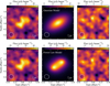 |
Fig. 2 Left column: same as the right panel in Fig. 1. Middle column: disk-only models created using RADMC-3D and tclean with the best-fit values from the MCMC fitting (see Table 2), as described in Sect. 4.2. Right column: residuals from subtracting the model visibilities from the data visibilities, as described in Sect. 4.3. Top row: Gaussian model and residuals corresponding to that model. Bottom row: power-law model and residuals corresponding to that model. All panels are imaged using a natural weighting and a u-v taper, as described in Sect. 2, and the contours are ±[2, 4, 6] × 10.4 µJy beam−1, the RMS noise level. |
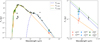 |
Fig. 3 Left: full multiwavelength photometry for HD 172555, including new mm photometry (colored symbols) from our observations. Right: zoom-in from the left panel focusing on ALMA (sub)mm data. In both panels, diamonds correspond to the higher spectral setup and squares correspond to the lower spectral setup. Dark orange markers are stellar fluxes, blue markers are disk fluxes, and dark green markers are total (disk and stellar) combined fluxes. Error bars are 1σ. Previous photometric measurements are in black, where circles are detections and downward-facing triangles are upper limits (photometric points are listed in Table B.1). The best-fit star (orange, solid) and single-component modified blackbody disk (blue, dash-dotted) models are included and obtained using the method from Yelverton et al. (2019). |
5 Discussion
5.1 Comparison with previous observations
In the mm, Schneiderman et al. (2021) detected the dust continuum and the 12CO J=2–1 transition, neither of which are spatially resolved. The 12CO is spectrally resolved and best described by a narrow ring of radius  au and width 3.4 ± 0.5 au. The dust is constrained to within 15 au of the star and is consistent with being co-located with the 12CO, both of which are consistent with our findings. Schneiderman et al. (2021) find a mm dust mass of (1.8±0.6) × 10−4 M⊕ from the observed continuum emission, assuming an equilibrium blackbody temperature of 169 K at ∼7.5 au and a dust grain opacity of 10 cm2 g−1 at 1000 GHz and scaling the dust grain opacity as κ ∝ νβ with β = 1 (Beckwith et al. 1990). For the 0.87 mm grains, we calculated a dust mass using the dust mass equation from Hildebrand (1983),
 (4)
where Mdust is the mass of the dust grains of a certain size in kg, Fν is the flux density of the dust grains in W m−1 Hz−1, d is the distance to HD 172555 in pc, κν is the opacity of the dust grains at the observation frequency in cm2 g−1, and Bν(T) is the Planck function at the frequency of the observation as a function of the temperature of the disk. Unlike the grains dominating the SED, we assumed the observed mm grains act as blackbodies. Using an equilibrium blackbody temperature of 213 K at 4.7 au, the median peak surface density radius found in the Gaussian model, and scaling the dust grain opacity as described above, we calculated a dust mass of (9.4±1.1) × 10−5 M⊕. When we instead used an equilibrium blackbody temperature of 191 K at 5.9 au, the mean of our best-fit (mode) values of Rin and Rout from the power-law mode, we calculated a dust mass of (10.5±1.2) × 10−5 M⊕, which is consistent with the dust mass calculated from the Gaussian model parameters. Our dust mass is lower than the dust mass calculated in Schneiderman et al. (2021) due to the higher temperature and smaller grains, and therefore lower opacities, considered here.
(4)
where Mdust is the mass of the dust grains of a certain size in kg, Fν is the flux density of the dust grains in W m−1 Hz−1, d is the distance to HD 172555 in pc, κν is the opacity of the dust grains at the observation frequency in cm2 g−1, and Bν(T) is the Planck function at the frequency of the observation as a function of the temperature of the disk. Unlike the grains dominating the SED, we assumed the observed mm grains act as blackbodies. Using an equilibrium blackbody temperature of 213 K at 4.7 au, the median peak surface density radius found in the Gaussian model, and scaling the dust grain opacity as described above, we calculated a dust mass of (9.4±1.1) × 10−5 M⊕. When we instead used an equilibrium blackbody temperature of 191 K at 5.9 au, the mean of our best-fit (mode) values of Rin and Rout from the power-law mode, we calculated a dust mass of (10.5±1.2) × 10−5 M⊕, which is consistent with the dust mass calculated from the Gaussian model parameters. Our dust mass is lower than the dust mass calculated in Schneiderman et al. (2021) due to the higher temperature and smaller grains, and therefore lower opacities, considered here.
In the FIR, in addition to atomic oxygen, Riviere-Marichalar et al. (2012) detected excesses from circumstellar dust at 70, 100, and 160 µm. Riviere-Marichalar et al. (2012) fit the excess with a modified blackbody model, yielding a temperature of 280±9 K, corresponding to a minimum blackbody dust radius of 2.7±0.2 au, which is in agreement with the location of the peak surface density in our observations within 1σ.
In the MIR, Smith et al. (2012) reanalyzed imaging taken with the Thermal-Region Camera Spectrograph (TReCS) at the Gemini South telescope, originally presented by Moerchen et al. (2010), to find that the warm dust emitting at ∼18 µm is in a disk with a median radius of 0.27″ (7.8 au) from the central star. They also modeled the visibilities from interferometric data taken with the MID-infrared Interferometric instrument (MIDI) on the Very Large Telescope Interferometer to place a lower limit of 1 au on the radial location of the emitting region (Smith et al. 2012). They did not detect extended emission in the TReCS imaging data at ∼11 µm, allowing them to place an upper limit of 0.27″ (7.8 au) on the spatial extent of the ∼11 µm emission. Because the ∼11 µm and ∼18 µm emission are at different locations, this indicates that this disk is extended, and the different bands of observation probe different regions of that disk due to their sensitivities to different temperatures (Smith et al. 2012). Also, in the MIR, Samland et al. (2025) detected atomic gas lines <0.5 au from the central star and note that the lines appear to trace evaporating dust, asteroids, or exocomets. The detected gas disk is much closer to the central star than the dust we detect. Samland et al. (2025) explore several options for the origin of the gas, including an evaporating population of close-in bodies, outgassing from a large in situ rocky planet, or the inward drift and sublimation of fine dust. It is therefore possible that dust produced in the impact could be responsible for the observed atomic gas emission (Samland et al. 2025; Su et al. 2020).
Scattered light observations (using a filter covering the R and I bands, with λc = 735 nm and ∆λ = 290 nm, Engler et al. 2018) indicate that the data are consistent with an axisymmetric dust disk with an outer radius between 0.3″ and 0.4″ (8.6–11.5 au). Engler et al. 2018 do not report a detection of an inner edge to the disk, but they note their observations do not probe interior to 5 au from the star. Furthermore, their data allow for the presence of compact emission closer to the star, behind the occulting spot of the coronagraph (Engler et al. 2018).
The findings from both scattered light and the MIR are consistent with our mm observations. Smith et al. (2012) reported that a disk position angle PA of 120◦ and an inclination i of 75◦ best fit their data, and placed the limits that 40◦ < PA <130◦ and i > 47◦. Engler et al. (2018) found a position angle of 112.3◦±1.5◦ and inclination of 76.2◦±1.7◦ best fit their data. The radial location and geometry of the disk in marginally resolved scattered light and MIR observations therefore indicate that small grains, as well as large mm-sized grains, are present in the same ≲11.5 au region from the central star.
5.2 Radial distribution
The results of our Gaussian model (Table 2, middle column) show that the disk is likely relatively broad, though not well constrained due to the S/N of our observations. In particular, our data exclude Gaussian models that are jointly compact (small R) and narrow (see joint R, ∆R probability distribution in Fig. A.1) because the emission is clearly resolved over several resolution elements in our images. Additionally, any peak surface density radii larger than ∼10 au were excluded because the detected emission only extends to ∼8.6 au. Overall, if we assume the Gaussian model, our data indicate that the surface mass density distribution is likely broader than a few au, with broader models peaking closer to the central star, and with no lower limit on a peak surface mass density distribution radius location, as emission is detected all the way to the central resolution element (Fig. 1). Even broader models beyond ∼8.6 au cannot be excluded if they are lower in surface brightness and therefore undetected at that boundary.
The results of our power-law model (Table 2, right column) show the disk is more likely to be relatively narrow, although, again, not well constrained due to the S/N of our observations. Rin is not constrained, although there is a marginally higher probability of Rin being larger, ∼5 au, rather than smaller (<3 au). While Rin, Rout pairs that span the range of the priors are allowed in the power-law model, there is a preference for narrower disks, as the joint Rin, Rout probability distribution peaks at larger Rin, ∼5 au, and smaller Rout, ∼7 au (see Fig. A.2). Overall, if we assume the power-law model, our data indicate that the surface mass density distribution is likely narrower and only a few au wide.
Our modeling results show that determining the radial extent of the HD 172555 dust disk is highly dependent on the model for the radial surface mass density distribution, highlighting the need for higher S/N observations. We note that parameters describing the radial surface density distribution of material are model-dependent; the rest (fluxes, i, PA, ∆RA, ∆Dec, and f ) are robust to changing model assumptions.
From MIR imaging, Smith et al. (2012) found that the observed emission can be fit by disks with radii from 0.09″ to 0.31″ (2.6–8.9 au) and widths between 0.36r and 2r, where r is the radius of the disk, implying that the grains probed by the ∼18 µm imaging have a broad distribution, which is supported by our Gaussian model results. Additionally, Lisse et al. (2009) fit the excess dust spectrum and modeled the grain composition to find that the small grains they observed, including the ones creating the silica feature at ∼9 µm, are 5.8±0.6 au from the central star. The location of the small grains from Lisse et al. (2009) produced in the impact are then consistent with the location of the mm grains.
In Fig. 4, the blue curve shows the normalized surface mass density, in arbitrary units, calculated from randomly sampled R, ∆R pairs from the Gaussian model MCMC samples. This curve shows the likely broad distribution of the mm dust in the HD 172555 disk the Gaussian model finds. The purple curve is the same as the blue one, but calculated using randomly sampled Rin, Rout, p triples from the power-law model MCMC samples. The orange curve in Fig. 4 is a scaled surface mass density obtained using the best-fit disk geometry and modeling parameters from the scattered light observations, where we converted from number density given by Engler et al. (2018) to surface mass density using their assumed vertical density structure. From these, it is clear that distributions of the mm grains and the smaller ones probed by the scattered light observations are offset, where the mm grains are closer to the star than the smaller grains, potentially by a factor of two, although there is a high uncertainty on this value.
Given the known presence of gas, the difference in the radial location of the grains could be due to radiation pressure with gas drag (e.g., Takeuchi & Artymowicz 2001). Both radiation pressure from the central star and gas drag affect grains of different sizes differently, causing them to potentially migrate inward or outward until the grains feel no net torque (Takeuchi & Artymowicz 2001). For radiation, it is helpful to compare how the forces of radiation and gravity affect a grain’s orbit. The ratio between radiation and gravity is β, which, from Burns et al. (1979), is given by
 (5)
where L∗ is the luminosity of the central star, QPR is the radiation pressure coefficient averaged over the stellar spectrum, M∗ is the mass of the central star, a is the radius of a grain, and ρd is the material density of the grain, all in SI units. From Eq. (5), it is clear smaller grains will feel a stronger force from the stellar radiation than larger grains and will therefore be pushed onto more eccentric orbits, creating a dust distribution where smaller grains are seen at larger orbital distances, assuming other frictional forces are negligible (Krivov 2010).
(5)
where L∗ is the luminosity of the central star, QPR is the radiation pressure coefficient averaged over the stellar spectrum, M∗ is the mass of the central star, a is the radius of a grain, and ρd is the material density of the grain, all in SI units. From Eq. (5), it is clear smaller grains will feel a stronger force from the stellar radiation than larger grains and will therefore be pushed onto more eccentric orbits, creating a dust distribution where smaller grains are seen at larger orbital distances, assuming other frictional forces are negligible (Krivov 2010).
In the presence of gas, a standard way to characterize the behavior of solids is with the Stokes number, which quantifies the extent to which a grain is affected by gas drag by comparing the stopping timescale ts to the orbital timescale  (e.g., Birnstiel et al. 2010). We express the Stokes number, St, as
 (6)
where ρg is the density of the gas, and vth is the thermal velocity of the gas.
(6)
where ρg is the density of the gas, and vth is the thermal velocity of the gas.
It is then possible for the combined effect of gas drag and radiation pressure from the central star, if the gas density ρg is high enough, to cause outward drift of the smaller grains without affecting the mm grains, if the Stokes numbers of each grain are right for those conditions. Without knowing the gas density, and therefore composition beyond CO, it is difficult to accurately determine the Stokes numbers for the grain sizes probed by these observations. Assuming the gas is dominated by CO as detected by Schneiderman et al. (2021), we take both the optically thick (∼38 K) and optically thin (169 K) CO masses they derived and find Stokes numbers in the range of 10−2–103 for micron-sized grains and 102–106 for mm-sized grains. It is therefore plausible, for the larger masses implied if 12CO is optically thick, or if other species dominate the gas mass, that the micron-sized grains drift outward while the mm grains would be unaffected. However, full radiative transfer gas modeling is needed for quantitative interpretation of the gas drag, as, for example, the mass and radial distribution of the 12CO detected by Schneiderman et al. (2021) are degenerate and model-dependent, respectively.
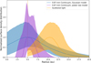 |
Fig. 4 Surface density distribution of the mm grains from this paper (Gaussian model in blue, power-law model in purple) compared to the surface density distribution from scattered light imaging (orange, Engler et al. 2018). The orange dashed line is the inner limit of the scattered light observations. All curves have been normalized to 1, and the shaded regions correspond to 1σ error. |
5.3 Mass of the largest impacting planet
Using the radial width of the disk of mm-sized grains, we can constrain the mass of the largest impacting planet, assuming gas has not impacted the dynamics of the mm and larger sized grains throughout the post-impact evolution. Following from Jackson et al. (2014), the radial width of the debris from a giant impact is directly related to the velocity dispersion of the debris. The debris is expected to be ejected from the impacting planetary embryos with relative velocities of order the escape velocities of the impactors, which makes the radial width of the grains the best proxy for progenitor mass. A more massive progenitor would have a higher escape velocity, which would result in a broader distribution of mm-sized grains compared to a less massive progenitor. From Schneiderman et al. (2021), the expected mass of the impacting planet in M⊕ is
 (7)
where M∗ is the stellar mass in M⊙, ρp is the bulk density of the planet in g cm−3, and R and ∆R are in au. Using M∗ = 1.76 M⊙, ρp = 5.5 g cm−3, and randomly sampled R, ∆R pairs from the Gaussian model MCMC samples, we derived a mass estimate of
(7)
where M∗ is the stellar mass in M⊙, ρp is the bulk density of the planet in g cm−3, and R and ∆R are in au. Using M∗ = 1.76 M⊙, ρp = 5.5 g cm−3, and randomly sampled R, ∆R pairs from the Gaussian model MCMC samples, we derived a mass estimate of  MJup. However, this estimate is not well constrained due to the high uncertainties on the mm dust radius and width from the Gaussian model (see Sect. 5.2). Additionally, a planet with this mass is likely to be a gas giant, which means that the outcome of a collision with such a planet is unlikely to be large amounts of dust, as we assumed.
We can also use the results from the power-law model to estimate the mass of the largest impacting planet. We randomly sampled Rin, Rout pairs from the power-law model MCMC. In Eq. (7), we take R to be the mean of the Rin and Rout and ∆R to be the difference between Rout and Rin. Again using M∗ = 1.76 M⊙ and ρp = 5.5 g cm−3, we derived an estimate of  M⊕ (
M⊕ ( MJup) for the mass of the largest impacting planet. A planet of this mass is likely to be a terrestrial planet, meaning the outcome of a collision with this planet would be consistent with our assumptions about the debris from the giant impact. While we cannot distinguish between the two models with our data, the mass of the largest impacting planet we derive using the Gaussian model is unlikely, while the mass derived using the power-law model is more consistent with our assumptions. This makes the power-law model physically preferable to the Gaussian model.
Although it is unclear how massive the largest impactor was, we can consider timescales for debris survival in the disk as it encounters a leftover planet (Wyatt et al. 2017). Conservatively, we assume that a leftover planet will have a mass of order the mass of the largest impactor. Using Eq. (2) from Brasser & Duncan (2008), with a semimajor axis of 4.7 au, the eventual outcome for debris encountering a planet of 0.5 MJup is ejection from the system, with an ejection timescale of ∼0.8 Myr. A less massive remaining planet would have a longer ejection timescale, and for planet masses below a certain threshold, the predominant outcome for debris encounters will be accretion. The eventual outcome for debris encountering a 4.5 M⊕ leftover planet at ∼5 au is accretion onto the remaining planet, although the accretion timescale is much longer than the age of the system. It remains possible that the mass of the largest impactor was ∼0.5 MJup, as long as we are observing this system within ∼0.8 Myr of the impact. It is also possible that the mass of the largest impacting planet was 4.5 M⊕, as debris would survive encounters with a leftover planet of order 4.5 M⊕ for longer than the age of the system.
We can also consider the limits on the presence of any planets in the system that may affect post-impact debris evolution. Quanz et al. (2011) used VLT/NACO to search for planetary mass companions to HD 172555 at 4 µm, and while they did not detect any planets, they derived detection limits of 2–3 MJup at projected separations of 15–29 au and ≳4 MJup at ∼11 au. Meunier et al. (2012) used radial velocity data to place detection limits of between ∼4 MJup for short period orbits (0.6 au) and ∼30–70 MJup for long period orbits (2.1 au).
While our derived impactor masses are within these observational limits, and while debris could survive repeat encounters with the more massive planet estimate up to ∼0.8 Myr post-impact, the currently large uncertainties, particularly on the mass derived using the results from the Gaussian model, prevent us from drawing firm conclusions. Deeper observations of gravitationally bound grains will be needed to better constrain the radial width of the debris and, by extension, the mass of the largest impacting planet.
5.4 Limits on potential asymmetry
Motivated by marginal evidence for an asymmetry in the dust distribution detected by Smith et al. (2012) and Engler et al. (2018), with the southeast side being brighter, we attempt to constrain the magnitude of an asymmetry in the mm by assuming that we would just be able to detect an asymmetry if the ratio of the peak intensity on each side of the disk was inconsistent with 1 by at least 3σ. Using the maximum intensity of (5.1±0.9) × 10−5 Jy beam−1 on the southeast side of the disk and (4.2±0.9) × 10−5 Jy beam−1 on the northwest side of the disk in the right panel of Fig. 1, we find that the ratio of the southeast intensity, Iν,SE, to the northwest intensity, Iν,NW, is 1.21±0.39, which is consistent with 1, implying that no southeast-northwest asymmetry is detected in our data. Detection would have only been achieved if  was 3σ above 1, or
  . = 2.17. We therefore constrain a possible asymmetry in the mm dust distribution to not more than a 117% difference between the southeast and northwest sides of the disk, assuming the asymmetry is in the plane of the sky. It is then plausible for a weak to moderate asymmetry to still be present for the mm grains and compatible with the marginal asymmetry seen in shorter wavelength observations (Engler et al. 2018; Smith et al. 2012).
Whether or not an asymmetry is present would allow us to constrain the time that has passed since the impact. The debris from a giant impact is produced at one point in space, which means that, in the absence of sufficient amounts of gas to affect the grain dynamics, all of the debris orbits start at this location and must pass through this point again (Jackson et al. 2014). Because all of the debris orbits must then pass through the impact point, the models show that this creates a pinch point in the disk with enhanced dust production from further collisions between debris produced in the impact, leading to an azimuthal asymmetry in the dust structure (Jackson et al. 2014). The asymmetry then smears out over time as the orbits precess from interactions with leftover planets, other planets in the system, or the post-impact disk’s own self-gravity, to eventually create an axisymmetric disk. The timescale for a disk to become centrally symmetric depends strongly on the semimajor axis of the debris, as well as on the semimajor axis and mass of planets with which the debris interacts, and could be of order a few tens of thousands of debris orbits (Jackson et al. 2014; Kral et al. 2015). In the HD 172555 system, this would translate to a timescale of ∼0.3 Myr for the disk to become symmetric. It is possible that we are observing this system ≳0.3 Myr post-impact, especially given the accretion timescale discussed in Sect. 5.3 if the mass of the largest impacting planet was of order 4.5 M⊕. In the high impactor mass scenario, given the debris ejection timescale discussed in Sect. 5.3, it is possible (although unlikely) that we are observing this system between ∼0.3 and ∼0.8 Myr post-impact. We cannot accurately constrain the time that has passed since the impact until the disk’s radial width and level of asymmetry are more accurately constrained with higher S/N observations.
6 Summary
In this work, we present the first spatially resolved 0.87 mm continuum observations of post-impact dust around HD 172555 obtained with ALMA. We imaged and modeled the interferometric visibilities of our data to analyze the disk structure. We report the following findings:
We clearly detected the star and the disk; after subtracting the star interferometrically, an inclined disk of mm dust emission is revealed, extending out to ∼9 au, and down to within 2.3 au of the star on-sky.
We measured mm fluxes implying a total dust mass of (9.4 ± 1.1) × 10−5 and we included the fluxes in SED modeling, revealing a spectral slope of 2.74 ± 0.03. This implies a size distribution slope of 3.41±0.05, which differs from the size distribution measured for micron-sized grains. This implies that there is a break in the grain size distribution shortward of mm-sized grains.
Modeling the visibilities indicates that the radial disk surface density distribution most likely peaks around ∼5 au, while the radial width inferred remains dependent on the model. Our Gaussian model is more likely a broad disk than a narrow ring, while our power-law model is more likely to be a narrow ring between ∼5 and ∼7 au.
We report a radial offset between the mm grains and the small grains traced by scattered light observations (peaking at ∼11 au). This could be due to the combined effect of radiation pressure and gas drag, if the gas density is high enough.
Assuming our best-fit values of disk radius and width (Gaussian model) or inner and outer radius (power-law model) leads to estimates of the largest impacting planet mass of 0.5 MJup and 4.5 M⊕, respectively. In the large planet case, the impact is unlikely to be dust dominated, as has been assumed, and had to be very recent, as the ejection timescale is very short; whereas in the smaller, terrestrial planet case, most of the debris could have avoided dynamical removal, even if the impact happened very early in the system’s lifetime. However, our estimates remain highly uncertain given the S/N of our observations.
We do not see significant evidence of an asymmetry in the dust distribution. However, a strong asymmetry of <117% between the southeast and northwest sides of the disk could still be present and have gone undetected.
Further work is needed to better understand the post-impact dynamics in this system. Higher S/N observations would allow us to better constrain the radial distribution of the gravitationally bound dust, which would in turn lead to tighter limits on the mass of the largest impactor and the time that has passed since the impact. Additionally, to ascertain whether the gas in the disk impacts the dust dynamics, higher S/N ALMA and scattered light dust observations are needed to more accurately constrain a radial offset between the two. In parallel, an upcoming in-depth analysis of the gas composition and distribution using this ALMA data will allow us to constrain the disk’s volatile content and dynamics, shedding light on the impacting bodies and the subsequent debris evolution.
Acknowledgements
ZR and LM acknowledge funding by the European Union through the E-BEANS ERC project (grant number 100117693). SM acknowledges funding by the Royal Society through a Royal Society University Research Fellowship (URF-R1-221669) and the European Union through the FEED ERC project (grant number 101162711). Views and opinions expressed are however those of the author(s) only and do not necessarily reflect those of the European Union or the European Research Council Executive Agency. Neither the European Union nor the granting authority can be held responsible for them. This paper makes use of the following ALMA data: ADS/JAO.ALMA#2022.1.00793.S. ALMA is a partnership of ESO (representing its member states), NSF (USA) and NINS (Japan), together with NRC (Canada), NSC and ASIAA (Taiwan), and KASI (Republic of Korea), in cooperation with the Republic of Chile. The Joint ALMA Observatory is operated by ESO, AUI/NRAO and NAOJ.
References
- Andrews-Hanna, J. C., Zuber, M. T., & Banerdt, W. B. 2008, Nature, 453, 1212 [Google Scholar]
- Beckwith, S. V. W., Sargent, A. I., Chini, R. S., & Guesten, R. 1990, AJ, 99, 924 [Google Scholar]
- Benz, W., Slattery, W. L., & Cameron, A. G. W. 1988, Icarus, 74, 516 [NASA ADS] [CrossRef] [Google Scholar]
- Benz, W., Anic, A., Horner, J., & Whitby, J. A. 2007, SSRv, 132, 189 [Google Scholar]
- Birnstiel, T., Dullemond, C. P., & Brauer, F. 2010, A&A, 513, A79 [NASA ADS] [CrossRef] [EDP Sciences] [Google Scholar]
- Brasser, R., & Duncan, M. J. 2008, Celest. Mech. Dyn. Astron., 100, 1 [Google Scholar]
- Briggs, D. S. 1995, Ph.D. thesis, New Mexico Institute of Mining and Technology, USA [Google Scholar]
- Burns, J. A., Lamy, P. L., & Soter, S. 1979, Icarus, 40, 1 [Google Scholar]
- Cameron, A. G. W., & Ward, W. R. 1976, Abstracts of the Lunar and Planetary Science Conference, 7, 120 [Google Scholar]
- Cameron, A. G. W., Benz, W., Fegley, B., Jr., & Slattery, W. L. 1988, in Mercury (University of Arizona Press), 692 [Google Scholar]
- Canup, R. M. 2004, Icarus, 168, 433 [NASA ADS] [CrossRef] [Google Scholar]
- Canup, R. M., & Asphaug, E. 2001, Nature, 412, 708 [Google Scholar]
- Chambers, J. E. 2001, Icarus, 152, 205 [Google Scholar]
- Chen, C. H., Sargent, B. A., Bohac, C., et al. 2006, ApJS, 166, 351 [NASA ADS] [CrossRef] [Google Scholar]
- Cote, J. 1987, A&A, 181, 77 [NASA ADS] [Google Scholar]
- Cutri, R. M., Skrutskie, M. F., van Dyk, S., et al. 2003, 2MASS All Sky Catalog of Point Sources (NASA/IPAC Infrared Science Archive) [Google Scholar]
- Dohnanyi, J. S. 1969, JGR, 74, 2531 [NASA ADS] [CrossRef] [Google Scholar]
- Draine, B. T. 2006, ApJ, 636, 1114 [Google Scholar]
- Dullemond, C. P., Juhasz, A., Pohl, A., et al. 2012, Astrophysics Source Code Library [record ascl:1202.015] [Google Scholar]
- Engler, N., Schmid, H. M., Quanz, S. P., Avenhaus, H., & Bazzon, A. 2018, A&A, 618, A151 [NASA ADS] [CrossRef] [EDP Sciences] [Google Scholar]
- ESA. 1997, ESA Special Publication, 1200 [Google Scholar]
- Foreman-Mackey, D., Hogg, D. W., Lang, D., & Goodman, J. 2013, PASP, 125, 306 [Google Scholar]
- Foreman-Mackey, D., Farr, W., Sinha, M., et al. 2019, JOSS, 4, 1864 [Google Scholar]
- Fujiwara, H., Onaka, T., Yamashita, T., et al. 2012, ApJ, 749, L29 [Google Scholar]
- Gaia Collaboration 2022, VizieR Online Data Catalog: I/355 [Google Scholar]
- Geiler, F., & Krivov, A. V. 2017, MNRAS, 468, 959 [Google Scholar]
- Goodman, J., & Weare, J. 2010, Commun. Appl. Math. Computat. Sci., 5, 65 [Google Scholar]
- Grady, C. A., Brown, A., Welsh, B., et al. 2018, AJ, 155, 242 [NASA ADS] [CrossRef] [Google Scholar]
- Gray, R. O., Corbally, C. J., Garrison, R. F., et al. 2006, AJ, 132, 161 [Google Scholar]
- Gáspár, A., Rieke, G. H., & Balog, Z. 2013, ApJ, 768, 25 [CrossRef] [Google Scholar]
- Helou, G., & Walker, D. W. 1988, Infrared Astronomical Satellite (IRAS) Catalogs and Atlases, 7, 1 [NASA ADS] [Google Scholar]
- Hildebrand, R. H. 1983, QJRAS, 24, 267 [NASA ADS] [Google Scholar]
- Hughes, A. M., Duchêne, G., & Matthews, B. C. 2018, ARA&A, 56, 541 [Google Scholar]
- Högbom, J. A. 1974, A&AS, 15, 417 [Google Scholar]
- Høg, E., Fabricius, C., Makarov, V. V., et al. 2000, A&A, 355, L27 [Google Scholar]
- IRSA, & SSC. 2020, Spitzer Enhanced Imaging Products, NASA IPAC DataSet,IRSA433 [Google Scholar]
- Ishihara, D., Onaka, T., Kataza, H., et al. 2010, A&A, 514, A1 [NASA ADS] [CrossRef] [EDP Sciences] [Google Scholar]
- Izidoro, A., & Raymond, S. N. 2018, Formation of Terrestrial Planets (Springer International Publishing AG) [Google Scholar]
- Jackson, A. P., Wyatt, M. C., Bonsor, A., & Veras, D. 2014, MNRAS, 440, 3757 [NASA ADS] [CrossRef] [Google Scholar]
- Johnson, B. C., Lisse, C. M., Chen, C. H., et al. 2012, ApJ, 761, 45 [NASA ADS] [CrossRef] [Google Scholar]
- Kennedy, G. M., & Wyatt, M. C. 2013, MNRAS, 433, 2334 [NASA ADS] [CrossRef] [Google Scholar]
- Kiefer, F., Lecavelier des Etangs, A., Augereau, J. C., et al. 2014, A&A, 561, L10 [NASA ADS] [CrossRef] [EDP Sciences] [Google Scholar]
- Kiefer, F., Van Grootel, V., Lecavelier des Etangs, A., The Herschel/PACS Point Source Catalogue Explanatory Supplement et al. 2023, A&A, 671, A25 [NASA ADS] [CrossRef] [EDP Sciences] [Google Scholar]
- Kral, Q., Thébault, P., Augereau, J. C., Boccaletti, A., & Charnoz, S. 2015, A&A, 573, A39 [NASA ADS] [CrossRef] [EDP Sciences] [Google Scholar]
- Krivov, A. V. 2010, Res. A&A, 10, 383 [Google Scholar]
- Lisse, C. M., Chen, C. H., Wyatt, M. C., et al. 2009, ApJ, 701, 2019 [NASA ADS] [CrossRef] [Google Scholar]
- MacGregor, M. A., Wilner, D. J., Chandler, C., et al. 2016, ApJ, 823, 79 [Google Scholar]
- Marino, S., Carpenter, J., Wyatt, M. C., et al. 2018, MNRAS, 479, 5423 [NASA ADS] [CrossRef] [Google Scholar]
- Marshall, J. P., Maddison, S. T., Thilliez, E., et al. 2017, MNRAS, 468, 2719 [NASA ADS] [CrossRef] [Google Scholar]
- Marton, G., Calzoletti, L., Perez Garcia, A. M., et al. 2017, The Herschel/PACS Point Source Catalogue Explanatory Supplement [Google Scholar]
- Matrà, L., Wyatt, M. C., Wilner, D. J., et al. 2019, AJ, 157, 135 [CrossRef] [Google Scholar]
- Matrà, L., Dent, W. R. F., Wilner, D. J., et al. 2020, ApJ, 898, 146 [CrossRef] [Google Scholar]
- Meng, H. Y. A., Rieke, G. H., Su, K. Y. L., et al. 2012, ApJ, 751, L17 [Google Scholar]
- Mermilliod, J. C. 2006, VizieR Online Data Catalog: II/168 [Google Scholar]
- Meunier, N., Lagrange, A. M., & De Bondt, K. 2012, A&A, 545, A87 [NASA ADS] [CrossRef] [EDP Sciences] [Google Scholar]
- Mittal, T., Chen, C. H., Jang-Condell, H., et al. 2015, ApJ, 798, 87 [Google Scholar]
- Moerchen, M. M., Telesco, C. M., & Packham, C. 2010, ApJ, 723, 1418 [Google Scholar]
- Morbidelli, A., Lunine, J. I., O’Brien, D. P., Raymond, S. N., & Walsh, K. J. 2012, AREPS, 40, 251 [Google Scholar]
- Olivares, J., Miret-Roig, N., Galli, P. A. B., & Bouy, H. 2025, A&A, 699, A122 [NASA ADS] [CrossRef] [EDP Sciences] [Google Scholar]
- Olofsson, J., Juhász, A., Henning, T., et al. 2012, A&A, 542, A90 [NASA ADS] [CrossRef] [EDP Sciences] [Google Scholar]
- Pahlevan, K., Stevenson, D. J., & Eiler, J. M. 2011, E & PSL, 301, 433 [Google Scholar]
- Paunzen, E. 2015, A&A, 580, A23 [NASA ADS] [CrossRef] [EDP Sciences] [Google Scholar]
- Prialnik, D., & Rosenberg, E. D. 2009, MNRAS, 399, L79 [NASA ADS] [CrossRef] [Google Scholar]
- Quanz, S. P., Kenworthy, M. A., Meyer, M. R., Girard, J. H. V., & Kasper, M. 2011, ApJ, 736, L32 [Google Scholar]
- Rhee, J. H., Song, I., & Zuckerman, B. 2008, ApJ, 675, 777 [Google Scholar]
- Ricci, L., Testi, L., Maddison, S. T., & Wilner, D. J. 2012, A&A, 539, L6 [NASA ADS] [CrossRef] [EDP Sciences] [Google Scholar]
- Riviere-Marichalar, P., Barrado, D., Augereau, J. C., et al. 2012, A&A, 546, L8 [NASA ADS] [CrossRef] [EDP Sciences] [Google Scholar]
- Samland, M., Henning, T., Caratti o Garatti, A., et al. 2025, ApJ, 989, 132 [Google Scholar]
- Schneiderman, T., Matrà, L., Jackson, A. P., et al. 2021, Nature, 598, 425 [NASA ADS] [CrossRef] [Google Scholar]
- Smith, D. E., Zuber, M. T., Solomon, S. C., et al. 1999, Science, 284, 1495 [Google Scholar]
- Smith, R., Wyatt, M. C., & Haniff, C. A. 2012, MNRAS, 422, 2560 [Google Scholar]
- Snodgrass, C., Agarwal, J., Combi, M., et al. 2017, A&ARv, 25, 5 [Google Scholar]
- Su, K. Y. L., Rieke, G. H., Malhotra, R., et al. 2013, ApJ, 763, 118 [NASA ADS] [CrossRef] [Google Scholar]
- Su, K. Y. L., Rieke, G. H., Melis, C., et al. 2020, ApJ, 898, 21 [NASA ADS] [CrossRef] [Google Scholar]
- Takeuchi, T., & Artymowicz, P. 2001, ApJ, 557, 990 [NASA ADS] [CrossRef] [Google Scholar]
- Tazzari, M., Beaujean, F., & Testi, L. 2018, MNRAS, 476, 4527 [Google Scholar]
- The CASA Team, Bean, B., Bhatnagar, S., et al. 2022, PASP, 134, 114501 [NASA ADS] [CrossRef] [Google Scholar]
- Wilhelms, D. E., & Squyres, S. W. 1984, Nature, 309, 138 [Google Scholar]
- Wright, E. L., Eisenhardt, P. R. M., Mainzer, A. K., et al. 2010, AJ, 140, 1868 [Google Scholar]
- Wyatt, M. C., Smith, R., Greaves, J. S., et al. 2007, ApJ, 658, 569 [NASA ADS] [CrossRef] [Google Scholar]
- Wyatt, M. C., Bonsor, A., Jackson, A. P., Marino, S., & Shannon, A. 2017, MNRAS, 464, 3385 [Google Scholar]
- Yelverton, B., Kennedy, G. M., Su, K. Y. L., & Wyatt, M. C. 2019, MNRAS, 488, 3588 [Google Scholar]
- Zuckerman, B., Song, I., Bessell, M. S., & Webb, R. A. 2001, ApJ, 562, L87 [NASA ADS] [CrossRef] [Google Scholar]
Appendix A MCMC results
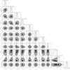 |
Fig. A.1 1D and 2D posterior probability distributions for all of the MCMC parameters from the Gaussian model (described in Sect. 4.1), where we applied a Gaussian prior to the inclination, i. Listed above each one-dimensional posterior probability distribution is the |

Appendix B Photometry
Photometric values
All Tables
All Figures
|
Fig. 1 Left: ALMA 0.87 mm continuum emission from the HD 172555 planetary system (star and disk) obtained by joint imaging of the combined visibility dataset. Right: same as the left panel, but imaged after removing the star from the visibilities, as described in Sect. 3. The symbol in the center notes the position of the star. In both panels, north is up and east is left. Contours are ±[2, 4, 6] × 10.4 µJy beam−1, the RMS noise level. Images are made with a natural weighting and a u-v taper, as described in Sect. 2. |
| In the text | |
|
Fig. 2 Left column: same as the right panel in Fig. 1. Middle column: disk-only models created using RADMC-3D and tclean with the best-fit values from the MCMC fitting (see Table 2), as described in Sect. 4.2. Right column: residuals from subtracting the model visibilities from the data visibilities, as described in Sect. 4.3. Top row: Gaussian model and residuals corresponding to that model. Bottom row: power-law model and residuals corresponding to that model. All panels are imaged using a natural weighting and a u-v taper, as described in Sect. 2, and the contours are ±[2, 4, 6] × 10.4 µJy beam−1, the RMS noise level. |
| In the text | |
|
Fig. 3 Left: full multiwavelength photometry for HD 172555, including new mm photometry (colored symbols) from our observations. Right: zoom-in from the left panel focusing on ALMA (sub)mm data. In both panels, diamonds correspond to the higher spectral setup and squares correspond to the lower spectral setup. Dark orange markers are stellar fluxes, blue markers are disk fluxes, and dark green markers are total (disk and stellar) combined fluxes. Error bars are 1σ. Previous photometric measurements are in black, where circles are detections and downward-facing triangles are upper limits (photometric points are listed in Table B.1). The best-fit star (orange, solid) and single-component modified blackbody disk (blue, dash-dotted) models are included and obtained using the method from Yelverton et al. (2019). |
| In the text | |
|
Fig. 4 Surface density distribution of the mm grains from this paper (Gaussian model in blue, power-law model in purple) compared to the surface density distribution from scattered light imaging (orange, Engler et al. 2018). The orange dashed line is the inner limit of the scattered light observations. All curves have been normalized to 1, and the shaded regions correspond to 1σ error. |
| In the text | |
|
Fig. A.1 1D and 2D posterior probability distributions for all of the MCMC parameters from the Gaussian model (described in Sect. 4.1), where we applied a Gaussian prior to the inclination, i. Listed above each one-dimensional posterior probability distribution is the |
| In the text | |
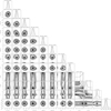 |
Fig. A.2 Same as Fig. A.1, but for the power-law model (described in Sect. 4.1). |
| In the text | |
Current usage metrics show cumulative count of Article Views (full-text article views including HTML views, PDF and ePub downloads, according to the available data) and Abstracts Views on Vision4Press platform.
Data correspond to usage on the plateform after 2015. The current usage metrics is available 48-96 hours after online publication and is updated daily on week days.
Initial download of the metrics may take a while.