| Issue |
A&A
Volume 706, February 2026
|
|
|---|---|---|
| Article Number | A336 | |
| Number of page(s) | 12 | |
| Section | Stellar atmospheres | |
| DOI | https://doi.org/10.1051/0004-6361/202557995 | |
| Published online | 20 February 2026 | |
Surface brightness–colour relations of Milky Way and Magellanic Clouds classical Cepheids based on Gaia magnitudes
1
Université Côte d’Azur, Observatoire de la Côte d’Azur, CNRS, Laboratoire Lagrange,
Nice,
France
2
Nicolaus Copernicus Astronomical Center, Polish Academy of Sciences,
ul. Bartycka 18,
00-716
Warszawa,
Poland
3
LIRA, Observatoire de Paris, Université PSL, Sorbonne Université, Université Paris Cité, CY Cergy Paris Université, CNRS,
5 place Jules Janssen,
92195
Meudon,
France
4
French-Chilean Laboratory for Astronomy,
IRL 3386, CNRS, Casilla 36-D,
Santiago,
Chile
5
Universidad de Concepción, Departamento Astronomía,
Casilla 160-C,
Concepción,
Chile
6
Leibniz Institute for Astrophysics,
An der Sternwarte 16,
14482
Potsdam,
Germany
7
Instituto de Alta Investigación, Universidad de Tarapacá,
Casilla 7D,
Arica,
Chile
★ Corresponding author: This email address is being protected from spambots. You need JavaScript enabled to view it.
Received:
6
November
2025
Accepted:
10
January
2026
Abstract
Context. Surface brightness–colour relations (SBCRs) are widely used to estimate the angular diameters of stars. In particular, they are employed in the Baade–Wesselink distance determination method, which relies on the comparison between the linear and angular amplitudes of Cepheids. The SBCR can be calibrated by combining different photometric systems. An SBCR was recently calibrated based on Gaia DR3 magnitudes alone for fundamental-mode classical Cepheids with solar metallicity. This relation appears to be strongly affected by metallicity, however.
Aims. We derive SBCRs for classical Cepheids in the Milky Way and in the Magellanic Clouds using the photometric data available in the Gaia database, and we quantify the metallicity effect.
Methods. We first selected the data on the basis of a number of quality criteria and chose the best photometric data and the best parallaxes available in Gaia for Milky Way classical Cepheids. Secondly, we compiled an extensive list of period–radius (PR) relations available in the literature, and we also provide a new PR relation based on interferometric data in our previous work. Thirdly, combining the radius of classical Cepheids with distance estimates (based on Gaia parallaxes for the Milky Way and on eclipsing binaries for the Magellanic Clouds), we derived the surface brightness and colour of about 1700 classical Cepheids.
Results. We first derived a new PR relation based on interferometric data and distances from the literature of seven classical Cepheids: log(R/R⊙) = 1.133±0.019 + 0.688±0.016log(P). The metallicity does not affect the PR relations. Secondly, we calculated three different SBCRs for the Milky Way and Large and Small Magellanic Cloud classical Cepheids based on this new PR relation that clearly show the dependence of the metallicity on the SBCR based on Gaia magnitudes alone. Finally, we derived relations between the slopes, the zero points (ZP), and the metallicity ([Fe/H]) of these three SBCRs: SlopeSBCR = −0.0663±0.0121[Fe/H] − 0.3010±0.0030 and ZPSBCR = −0.1016±0.0091 [Fe/H] + 3.9988±0.0029.
Conclusions. These new SBCRs, dedicated to classical Cepheids in the Milky Way and Magellanic Clouds, are of particular importance to apply the inverse Baade–Wesselink method to classical Cepheids observed by Gaia in a forthcoming study.
Key words: techniques: interferometric / stars: atmospheres / stars: distances / stars: fundamental parameters / stars: variables: Cepheids / Magellanic Clouds
© The Authors 2026
 Open Access article, published by EDP Sciences, under the terms of the Creative Commons Attribution License (https://creativecommons.org/licenses/by/4.0), which permits unrestricted use, distribution, and reproduction in any medium, provided the original work is properly cited.
This article is published in open access under the Subscribe to Open model. This email address is being protected from spambots. You need JavaScript enabled to view it. to support open access publication.
1 Introduction
The surface brightness–colour relation (SBCR) is commonly used to determine the angular diameter of stars based on their photometric measurements in two different bands. These relations are used, for example, in studies of exoplanet host stars (Gent et al. 2022; Di Mauro et al. 2022) or asteroseismic targets (Valle et al. 2024; Campante et al. 2019). They were also used to derive the distance of eclipsing binaries in the Large (Pietrzyński et al. 2013, 2019) and Small Magellanic Clouds (Graczyk et al. 2020) with an unprecedented accuracy of 1 and 2%, respectively, which is of particular importance for the determination of the Hubble-Lemaitre constant (Riess et al. 2022, 2024; Di Valentino et al. 2025). The SBCR is also used in the context of the Baade–Wesselink (BW) method of Cepheid distance determinations (Wesselink 1969). The BW method (or parallax of pulsation method) compares the linear and angular dimensions of Cepheids to derive its distance (Kervella et al. 2004c; Gieren et al. 2018; Mérand et al. 2015). Salsi et al. (2022) has shown theoretically based on atmospheric models that SBCRs depend not only on the temperature, but also on their luminosity class. When the BW method is applied to Cepheids, an SBCR dedicated to Cepheids is therefore required, in particular because the BW method is very sensitive to the choice of the SBCR (Nardetto et al. 2023). One of the largest current photometric survey of Cepheids is the Gaia survey, which has observed thousands of Cepheids in three different passbands (Gaia Collaboration 2016; Rimoldini et al. 2022). Recently, Bailleul et al. (2025) have calibrated a new SBCR based on Gaia bands alone that is dedicated to classical Cepheids (hereafter, Cepheids refers to fundamental-mode classical Cepheids), which opens the road to the application of the BW method to thousands of Cepheids in the Gaia database. We also found in this study that the SBCR is highly sensitive to metallicity, however, which limits its application.
In this work, we calibrate the SBCR in the Gaia photometric bands GBP and GRP for Milky Way (MW) and Magellanic Cloud (MC) Cepheids for the first time using an inverse method in which the radius is estimated from a period–radius (PR) relation, while the distance is based on Gaia parallaxes for the MW Cepheids and eclipsing binaries for the MC Cepheids. The paper is structured as follows. In Sect. 2, we present the selection process on the Gaia data. In Sect. 3, we present a compilation of PR relations and a new PR relation derived from interferometric measurements and various distance estimates that is then specifically used to calibrate the SBCR. In Sect. 4, we discuss the corrections applied to the Gaia parallaxes and the choice of distances to the Magellanic clouds. We then present the method we applied to the photometric data from Gaia and the extinction we used to correct for them in the Sections 5 and 6. We discuss the metallicity of the MW and MC Cepheids in Sect. 7. Finally, we present in Sect. 8 the SBCRs we found for MW and the MC Cepheids and conclude.
2 Data selection
We retrieved the light curves in the GBP and GRP magnitude bandpasses of all Cepheids from the Gaia DR3 database, as well as some specific parameters (Gaia Collaboration 2022, 2023a; Gaia Collaboration 2023b). We are particularly interested in the following parameters: type, mode, parallax, parallax error, period, and the renormalised unit weight error (RUWE). The selection process is described in Fig. 1. We first selected the DCEP (corresponds to classical Cepheids in the Gaia classification) and FUNDAMENTAL Cepheids. This first study is devoted to classical Cepheids alone because they have been extensively observed by interferometry in the past decades, which is not the case for first-overtone or anomalous Cepheids. This helped us to first apply our method consistently because we used a PR relation based on interferometry (see Sect. 3), and it also allowed us to compare our result with a direct recent calibration of the SBCR by interferometry (see Sect. 8). Secondly, we rejected poor-quality photometry using three flags: variability_flag_bp_reject, variability_flag_rp_reject,rejected_by_photometry. Third, we selected only stars with a good phase coverage, which means at least one measurement per bin in 0.1 in phase. This minimum coverage ensured that we derived a robust mean magnitude (see Sect. 5). To derive the pulsation phase, we used the following method: We phased the data using the observation time given by the catalogue for each band (i.e. bp_obs_time and rp_obs_time) and using ![Mathematical equation: $\[\phi_{\mathrm{i}}=\frac{\mathrm{JD}_{\mathrm{i}}{-}\mathrm{T}_{0}}{\mathrm{P}_{\text {ref}}}(\bmod 1)\]$](/articles/aa/full_html/2026/02/aa57995-25/aa57995-25-eq1.png) , where T0 is the reference epoch, and Pref is the pulsation period. Fourth, we selected the stars whose relative parallax error was smaller than 10%. To be consistent with the grid of the G-Tomo extinction maps discussed in Sect. 6, we removed Cepheids whose distances were smaller than 5 kpc and whose absolute height (z) relative to the Galactic plane exceeded 400 pc. This selection focused on Galactic Cepheids located in the plane in the Solar vicinity. We note that this selection biased our Cepheid sample towards a shorter pulsation period since their long-period counterparts are mostly found closer to the Galactic centre beyond 5 kpc. For the MW Cepheids, our period ranged between 2 and 45 days, with a median of 5.7 days. In addition, we set an upper limit on the RUWE indicator to 1.4. This parameter gives information about the quality of the fit of the astrometric observations, and a value higher than 1.4 might indicate that the source is not single or that there is a problem for the astrometric solution (Lindegren et al. 2021). Fifth, we selected Large Magellanic Cloud (LMC) and Small Magellanic Cloud (SMC) stars within a radius of 3° and 0.6°, respectively, around the centre of the clouds in order to limit the distance dispersion of these stars (see Sect. 4). Sixth, some stars were removed according to the limits of the extinctions maps we used and the availability of extinction values (see Sect. 6). Finally, we rejected all the Cepheids that did not follow the period–Wesenheit (PW) relation as described in Sect. 8. At the end, we obtain 9.5%, 38.6%, and 24.0% of the total sample of DCEP and FUNDAMENTAL Cepheids available in the Gaia database for the Milky Way, LMC, and SMC, respectively. The whole selected sample is also visible in Fig. 2 in terms of right ascension and declination.
, where T0 is the reference epoch, and Pref is the pulsation period. Fourth, we selected the stars whose relative parallax error was smaller than 10%. To be consistent with the grid of the G-Tomo extinction maps discussed in Sect. 6, we removed Cepheids whose distances were smaller than 5 kpc and whose absolute height (z) relative to the Galactic plane exceeded 400 pc. This selection focused on Galactic Cepheids located in the plane in the Solar vicinity. We note that this selection biased our Cepheid sample towards a shorter pulsation period since their long-period counterparts are mostly found closer to the Galactic centre beyond 5 kpc. For the MW Cepheids, our period ranged between 2 and 45 days, with a median of 5.7 days. In addition, we set an upper limit on the RUWE indicator to 1.4. This parameter gives information about the quality of the fit of the astrometric observations, and a value higher than 1.4 might indicate that the source is not single or that there is a problem for the astrometric solution (Lindegren et al. 2021). Fifth, we selected Large Magellanic Cloud (LMC) and Small Magellanic Cloud (SMC) stars within a radius of 3° and 0.6°, respectively, around the centre of the clouds in order to limit the distance dispersion of these stars (see Sect. 4). Sixth, some stars were removed according to the limits of the extinctions maps we used and the availability of extinction values (see Sect. 6). Finally, we rejected all the Cepheids that did not follow the period–Wesenheit (PW) relation as described in Sect. 8. At the end, we obtain 9.5%, 38.6%, and 24.0% of the total sample of DCEP and FUNDAMENTAL Cepheids available in the Gaia database for the Milky Way, LMC, and SMC, respectively. The whole selected sample is also visible in Fig. 2 in terms of right ascension and declination.
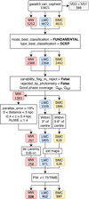 |
Fig. 1 Data selection process. |
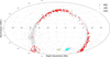 |
Fig. 2 Gaia all-sky view of the Milky Way and the Large and Small Magellanic Clouds. We show the total sample in grey. The final selected sample of Cepheids is shown in colour. |
3 Period–radius relations
In this section, we compile the PR relations available in the literature for Cepheids (see Table 1) based on the BW and CORS methods and on theory. In Sect. 3.1, we derive a new relation that is purely observational and is based on the interferometric dataset provided by Bailleul et al. (2025).
3.1 The BW method
The Baade–Wesselink (BW) method was first proposed by Lindemann (Lindemann 1918) based on the idea of verifying the pulsation hypothesis of variable stars. It was later put into practice by van Hoof (van Hoof 1945), who first applied it to calculate the distance of three Cepheids, and later by Wesselink (Wesselink 1969). The principle is as follows: The distance (d) of a pulsating star can be deduced by measuring the limb-darkened angular diameters (θLD) over the entire pulsation cycle and comparing them to the variation in stellar radius (ΔR) deduced from the integration of the radial velocity and using a projection factor (Nardetto et al. 2004). We then have
![Mathematical equation: $\[\theta_{\mathrm{LD}}=\bar{\theta}_{\mathrm{LD}}+\frac{\Delta \mathrm{R}}{\mathrm{~d}}.\]$](/articles/aa/full_html/2026/02/aa57995-25/aa57995-25-eq2.png) (1)
(1)
By fitting this relation, we can determine the distance and mean dimension of the star (![Mathematical equation: $\[\bar{\theta}_{\mathrm{LD}}\]$](/articles/aa/full_html/2026/02/aa57995-25/aa57995-25-eq3.png) and
and ![Mathematical equation: $\[\bar{\mathrm{R}}\]$](/articles/aa/full_html/2026/02/aa57995-25/aa57995-25-eq4.png) ). There are three different versions of the BW method, depending on how the variation in the angular diameter is determined: first, directly by interferometry (Kervella et al. 2004c), second, using an SBCR (Storm et al. 2011), and third, using the method called spectro-photo-interferometry for pulsating star (SPIPS) (Mérand et al. 2015), which combines several photometric bands, velocimetry, interferometry, and surface brightness derived using ATLAS9 atmospheric models (Castelli & Kurucz 2003). In this version, the authors computed a global fit of all the Cepheid parameters to derive its physical parameters (Gallenne et al. 2017; Trahin et al. 2021). Laney & Stobie (1995) used a slightly different method that was still based on the BW concepts. Introduced by Balona (1977), this method solely relies on the magnitude–colour diagram in the infrared domain, for which the light curves are entirely dominated by variations in the stellar radius. They derived the average radius using a maximum likelihood method. In the first part of Table 1, we list the PR relation found in the literature for which the BW method was used to derive the mean stellar radius of the Cepheids. We considered Fernie (1984), who compiled PR relations, PR relations that used an SBCR (Moffett & Barnes 1987; Rojo Arellano & Arellano Ferro 1994; di Benedetto 1994; Gieren et al. 1999; Groenewegen 2013; Gallenne et al. 2017), PR relations for which θLD was derived using direct interferometry (Kervella et al. 2004a; Groenewegen 2007), and different versions of the BW method (Laney & Stobie 1995; Turner & Burke 2002; Trahin et al. 2021).
). There are three different versions of the BW method, depending on how the variation in the angular diameter is determined: first, directly by interferometry (Kervella et al. 2004c), second, using an SBCR (Storm et al. 2011), and third, using the method called spectro-photo-interferometry for pulsating star (SPIPS) (Mérand et al. 2015), which combines several photometric bands, velocimetry, interferometry, and surface brightness derived using ATLAS9 atmospheric models (Castelli & Kurucz 2003). In this version, the authors computed a global fit of all the Cepheid parameters to derive its physical parameters (Gallenne et al. 2017; Trahin et al. 2021). Laney & Stobie (1995) used a slightly different method that was still based on the BW concepts. Introduced by Balona (1977), this method solely relies on the magnitude–colour diagram in the infrared domain, for which the light curves are entirely dominated by variations in the stellar radius. They derived the average radius using a maximum likelihood method. In the first part of Table 1, we list the PR relation found in the literature for which the BW method was used to derive the mean stellar radius of the Cepheids. We considered Fernie (1984), who compiled PR relations, PR relations that used an SBCR (Moffett & Barnes 1987; Rojo Arellano & Arellano Ferro 1994; di Benedetto 1994; Gieren et al. 1999; Groenewegen 2013; Gallenne et al. 2017), PR relations for which θLD was derived using direct interferometry (Kervella et al. 2004a; Groenewegen 2007), and different versions of the BW method (Laney & Stobie 1995; Turner & Burke 2002; Trahin et al. 2021).
Following Bailleul et al. (2025), we also derived a new period–radius relation for MW Cepheids and derived the mean value of the angular diameter directly from the observed interferometric angular diameter curves, combined with a distance based on various estimates in the literature (listed in Table 2). For the seven Cepheids presented by Bailleul et al. (2025), we first fitted the limb-darkened angular diameter curves using a second-order polynomial fit, and we estimated the error associated with the mean value using a bootstrapping method. The errors associated with the mean angular diameter, the dispersion in distance, and the errors associated with each distance were taken into account in the calculation of the error on the mean radius. The logarithm of the radius is plotted as a function of the period derived from Trahin et al. (2021) in Fig. 3. To fit the relation, we used a least-squares fitting method that considered uncertainties on the y-axis and the barycenter of the data points. In this method, the result initially had the following formalism: ![Mathematical equation: $\[\mathrm{y}=\alpha(x-\bar{x})+\beta\]$](/articles/aa/full_html/2026/02/aa57995-25/aa57995-25-eq5.png) . We then converted the relation into y = ax + b using a = α and
. We then converted the relation into y = ax + b using a = α and ![Mathematical equation: $\[b=-\alpha \bar{x}+\beta\]$](/articles/aa/full_html/2026/02/aa57995-25/aa57995-25-eq6.png) , and we derived the uncertainties from the covariance matrix (C) provided by the fitting routine as
, and we derived the uncertainties from the covariance matrix (C) provided by the fitting routine as ![Mathematical equation: $\[\sigma_{a}=\sqrt{C_{00}}, \sigma_{b}=\sqrt{\bar{x}^{2} C_{00}+C_{11}-2 \bar{x} C_{01}}\]$](/articles/aa/full_html/2026/02/aa57995-25/aa57995-25-eq7.png) . We obtained the following relation (see also Fig. 3):
. We obtained the following relation (see also Fig. 3):
![Mathematical equation: $\[\log \left(\mathrm{R} / \mathrm{R}_{\odot}\right)=0.688_{ \pm 0.038} \log (\mathrm{P})+1.133_{ \pm 0.044}.\]$](/articles/aa/full_html/2026/02/aa57995-25/aa57995-25-eq8.png) (2)
(2)
with a root mean square (RMS) of 0.015. This relation agrees very well with previous empirical relations from the BW method (Gieren et al. 1999; Groenewegen 2013; Gallenne et al. 2017) and with theoretical predictions for MW stars (Fernie 1984; Bono et al. 1998; Alibert et al. 1999; Petroni et al. 2003).
Period-radius relations from the literature.
3.2 The CORS method
The CORS method, named after its authors (Caccin, Onnembo, Russo and Sollazo; Caccin et al. 1981), is based on the same hypothesis as the BW method, with the difference that it allows us to determine the radius (instead of the radius variation in BW) of the Cepheids over the pulsation cycle. The method introduces a term ΔB, however, that is directly related to the surface brightness of Cepheids throughout the cycle. In the original CORS method, the ΔB term was neglected. Later studies (Sollazzo et al. 1981; Ripepi et al. 1997) showed that the radius can be determined better when this term is taken into account. The method was then modified by including the ΔB term using either the SBCR derived by Barnes & Evans (1976) (Ripepi et al. 1997) or using theoretical grids of effective temperature (Ruoppo et al. 2004; Molinaro et al. 2012a). All the PR relations associated with this method are listed in the second part of Table 1.
Distances in parsec of seven Cepheids from the literature.
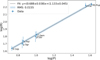 |
Fig. 3 Period-radius relation using data of seven Cepheids based on the interferometric angular diameter curve of Bailleul et al. (2025). |
3.3 Theoretical method
By combining stellar models with a theory of stellar pulsation, one can derive a theoretical radius for Cepheids that takes the stellar parameters of the stars into account, such as the effective temperature, the mass, or the luminosity class. Many authors used this (Karp 1975; Cogan 1978; Fernie 1984; Petroni et al. 2003; De Somma et al. 2022) with different stellar pulsation and evolution codes. Taking into account the metallicity, Bono et al. (1998) and Alibert et al. (1999) also derived theoretical PR relations for LMC and SMC stars. All these PR relations are listed in the third part of Table 1.
In addition, we note that Pilecki et al. (2018) derived completely independent radius measurements from double-lined eclipsing binaries in the LMC. Their method is very promising and provided the radii of three fundamental-mode Cepheids, which is not sufficient to fit the data and obtain an accurate relation on our side. Furthermore, the authors did not provide a PR relation.
In Fig. 4, we compare the slope and the zero point of all the PR relations listed in Table 1. The blue points show PR relations for LMC Cepheids, the orange ones for SMC Cepheids while the red points are all the PR relations for MW Cepheids. The three black dots correspond to PR relations that are valid for the three galaxies. The green diamond is the PR relation derived in this work. The slope and zero point are correlated, which is due to the fitting method used in these studies, which does not take the barycenter of the measurements into account. Importantly, we find no evidence that these relations depend on metallicity.
There is also no evidence in the literature that the PR relation depends on metallicity. Gallenne et al. (2017) derived a period–radius (PR) relation for MW, LMC, and SMC Cepheids and found no effect of the metallicity on the relation. This was also an important conclusion of Gieren et al. (1999) based on the SBCR approach.
4 Distances
For the Cepheids in the Milky Way, we adopted the parallaxes from Gaia EDR3 (Gaia Collaboration 2020) and inverted them to obtain the Cepheid distances. As explained in Sect. 2, since we restricted the sample to stars with parallax uncertainties below 10%, inverting the parallax to estimate the distance is approximately unbiased over this range (Bailer-Jones et al. 2021). A correction was applied to all parallaxes according to Lindegren et al. (2021), however. We used a dedicated Python code1 to derive all the zero-point offsets for the different MW Cepheids in our sample. As described by Lindegren et al. (2021), interpolations were only calibrated in the following ranges: 6 < phot_g_mean_mag < 21, 1.1 < nu_eff_used_in_astrometry < 1.9 and 1.24 < pseudocolour < 1.72. Only two Cepheids fell outside these intervals and were therefore rejected from the sample. We found an average parallax offset of −0.02 mas, which corresponds to a distance closer to the Cepheids of 185 pc on average (see Fig. 5). This value agrees with the global parallax bias measured from quasars (−17 μas) mentioned by Gaia Collaboration (2023b). We also compared our distance determination to the distances of Bailer-Jones (2023) and found a negligible median difference of 13.98 parsecs.
For LMC and SMC Cepheids, the distances from Gaia parallaxes are not accurate enough. We chose to fix the distance to the distances derived from eclipsing binaries by Pietrzyński et al. (2013, 2019) for the LMC and by Graczyk et al. (2020) for the SMC. We selected the stars that were included within a radius around the clouds centre. This was done to mitigate the effect of the 3D geometry of the Magellanic Clouds. We took as coordinates those used in the two papers cited above: α0 (LMC) = 80.05°, δ0 (LMC) = −69.3° and α0 (SMC) = 12.54°, δ0 (SMC) = −73.11°. Following the same method as Breuval et al. (2021), we used a radius of 3° for the LMC and 0.6° for the SMC (see Fig. 6). This selection represents a diameter of 1.3 kpc and 5.2 kpc around the respective centres of the SMC and LMC. We then added a correction to the distance of each star, assuming the geometry of the clouds, but also the elongated shape of the SMC (Jacyszyn-Dobrzeniecka et al. 2016; Graczyk et al. 2020), following the method of Breuval et al. (2021).
After this selection, 1095 and 628 Cepheids remained for the LMC and SMC, respectively, representing 46% and 25% of the DCEP and FUNDAMENTAL Cepheids in the two galaxies.
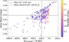 |
Fig. 5 Gaia zero-point offset as a function of the distance difference that it implies. The colour represents the parallax. Only the 228 selected Cepheids (after the whole selection process shown in Fig. 1) are shown here. |
5 Surface brightness–colour relation
As highlighted by Wesselink (1969), the surface brightness Sλ (the flux density received per unit of solid angle) of a star can be directly related to its limb-darkened angular diameter θLD, and its apparent magnitude corrected for the extinction mλ0 with the following formula:
![Mathematical equation: $\[\mathrm{S}_\lambda=\mathrm{m}_{\lambda_0}+5 ~\log \left(\theta_{\mathrm{LD}}\right).\]$](/articles/aa/full_html/2026/02/aa57995-25/aa57995-25-eq28.png) (3)
(3)
Barnes & Evans (1976) later determined a linear relation between the surface brightness (called Fλ) and the stellar colour index expressed in magnitude. Then, Fouque & Gieren (1997) derived the following relation:
![Mathematical equation: $\[\mathrm{F}_\lambda=4.2196-0.1 \mathrm{m}_{\lambda_0}-0.5 ~\log \left(\theta_{\mathrm{LD}}\right),\]$](/articles/aa/full_html/2026/02/aa57995-25/aa57995-25-eq29.png) (4)
(4)
where 4.2196 is a constant that depends on the solar parameters (Mamajek et al. 2015). For the first time, Bailleul et al. (2025) derived an SBCR dedicated to Cepheids using the GBP and GRP bands of the Gaia DR3 catalogue. We derived inverse SBCRs for MW, LMC and SMC Cepheids for the same combination of colours. The mean limb-darkened angular diameter (in milliarcseconds) was derived as follows:
![Mathematical equation: $\[\overline{\theta_{\mathrm{LD}}}=9.298 \frac{\overline{\mathrm{R}}}{\mathrm{~d}},\]$](/articles/aa/full_html/2026/02/aa57995-25/aa57995-25-eq30.png) (5)
(5)
where d is the distance in parsec (see Sect. 4), and ![Mathematical equation: $\[\bar{\text{R}}\]$](/articles/aa/full_html/2026/02/aa57995-25/aa57995-25-eq31.png) is the mean stellar radius in solar radii (from the PR relations; see Sect. 3). The constant comes from the conversion between these units. We then obtained the mean surface brightness (e.g., in the GBP band) using
is the mean stellar radius in solar radii (from the PR relations; see Sect. 3). The constant comes from the conversion between these units. We then obtained the mean surface brightness (e.g., in the GBP band) using
![Mathematical equation: $\[\mathrm{F}_{\mathrm{G}_{\mathrm{BP}}}=4.2196-0.1\left(\mathrm{~m}_{\mathrm{G}_{\mathrm{BP}}}\right)_0-0.5 ~\log _{10}\left(\overline{\theta_{\mathrm{LD}}}\right).\]$](/articles/aa/full_html/2026/02/aa57995-25/aa57995-25-eq32.png) (6)
(6)
The colour of a star can be defined simply as the difference between two dereddened apparent magnitudes measured in two different photometric bands. For our purpose, we used the dereddened average magnitude in the GBP and GRP bands. There are different possibilities regarding the way we derive the mean value of the magnitude over the pulsating cycle of the star. In Gaia, zpmagBP and zpmagRP are zero points in mag of the final model of the GBP and GRP band light curves (LCs). In other words, these values correspond to the zero point of the Fourier adjustments of the LCs. No uncertainties are available for these values, however. BPmagavg and RPmagavg are intensity-averaged magnitudes for which we have a dedicated uncertainty. In the Gaia source catalogue, phot_bp_mean_mag and phot_rp_mean_mag are defined as the mean magnitudes in the integrated GBP and GRP band, and they are computed from the GBP and GRP band mean flux applying the magnitude zero point in the Vega scale. They lack an associated uncertainty. We chose to use the values zpmagBP and zpmagRP instead because they are robustly determined from the LCs Fourier fit when the phase coverage is sufficient. To do this, we only considered stars with at least one measurement per bin of 0.1 in phase (see Sect. 2). We emphasize here that only considering an average magnitude of the data points is not enough because it is biased in some cases by the phase coverage (even when we considered a minimum of one measurement per bin of 0.1 in phase). The uncertainty on the mean value of the magnitude was calculated as the average of the uncertainties associated with each point on the curve, however.
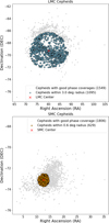 |
Fig. 6 LMC and SMC Cepheids within 3 and 0.6 degrees, respectively, from the clouds centre. |
6 Extinction
First, we tried to use the code G-Tomo (Lallement et al. 2022) that is available on GitHub2 to derive the extinction of all the stars, considering the coordinate of the star and its distance as input (following the method described in Sect. 4). More precisely, we decided to use the different extinction maps from Vergely et al. (2022) depending on the resolution, the limit in kiloparsec, and the distance of each star. We also rejected all the stars whose distances were larger than 5 kpc following the limit of the largest map. We finally found the extinction to be poorly estimated for a large number of Cepheids because their position did not follow the instability strip (IS). We chose to use the extinction values (E(GBP − GRP)) from de Laverny et al. (in prep., priv. commun.), derived from the GSPspec/DR3 stellar atmospheric parameters (Recio-Blanco et al. 2023). These extinctions were estimated by comparing the observed Gaia DR3 (GBP − GRP) colour with theoretical colours computed based on Gaia spectroscopic data. We used the following equation to convert E(GBP − GRP) into E(B − V): E(B − V) = E(GBP − GRP)/1.392 (Riello et al. 2021). The comparison between G-Tomo and de Laverny is given in Fig. 7 and confirms the better estimates by this second work. We plot the theoretical position of the red and blue edge of the IS found in De Somma et al. (2022) for Z=0.008 and Z=0.03 in a Hertzsprung-Russell (HR) diagram. We used table 1 of Mucciarelli et al. (2021) for giant stars to derive the effective temperature (Teff) from the de-reddened colours. The luminosity was calculated as follows: ![Mathematical equation: $\[\log _{10}\left(\frac{\mathrm{~L}}{\mathrm{~L}_{\odot}}\right)=0.4\left(\mathrm{M}_{\mathrm{G}, \odot}-\mathrm{M}_{\mathrm{G}}\right)\]$](/articles/aa/full_html/2026/02/aa57995-25/aa57995-25-eq33.png) , with MG = mG − 2.70 × E(B − V) − 5 log10(d) + 5. To derive the extinction coefficients, we used the following formulas from Ripepi et al. (2019):
, with MG = mG − 2.70 × E(B − V) − 5 log10(d) + 5. To derive the extinction coefficients, we used the following formulas from Ripepi et al. (2019):
![Mathematical equation: $\[\mathrm{A}_{\mathrm{G}}=2.70 ~\mathrm{E}(\mathrm{~B}-\mathrm{V})\]$](/articles/aa/full_html/2026/02/aa57995-25/aa57995-25-eq34.png) (7)
(7)
![Mathematical equation: $\[\mathrm{A}_{\mathrm{G}_{\mathrm{BP}}}=3.50 ~\mathrm{E}(\mathrm{~B}-\mathrm{V})\]$](/articles/aa/full_html/2026/02/aa57995-25/aa57995-25-eq35.png) (8)
(8)
![Mathematical equation: $\[\mathrm{A}_{\mathrm{G}_{\mathrm{RP}}}=2.15 ~\mathrm{E}(\mathrm{~B}-\mathrm{V}).\]$](/articles/aa/full_html/2026/02/aa57995-25/aa57995-25-eq36.png) (9)
(9)
For MC Cepheids, we used the result of Wang & Chen (2023), who derived the total-to-selective extinction ratio for red supergiants and classical Cepheids: RV(LMC) = 3.40 ± 0.07 and RV(SMC) = 2.53 ± 0.10, and the extinction maps from Górski et al. (2020), who reported E(B − V) (see Fig. 8).
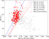 |
Fig. 7 HR diagram for MW Cepheids and position of the red and blue edge of the theoretical IS for Z=0.03 (dashed line) and Z=0.008 (dotted line). |
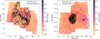 |
Fig. 8 LMC (left) and SMC (right) extinction maps (RA vs. Dec) from Górski et al. (2020) with matched Cepheids from our sample. The colour map indicates the value of E(B − V) at a certain location. |
7 Metallicity
We mainly considered three populations of Cepheids: those in the MW, LMC, and SMC. In order to study the metallicity effect on the SBCRs, we estimated the mean Cepheid metallicity in our sample using recent estimates in the literature.
Hocdé et al. (2023) gathered different determinations of the spectroscopic Cepheid metallicity from different sources and re-scaled them to the solar abundance value of A(Fe) = 7.50 (Asplund et al. 2009). This compilation is based on the largest dataset with a homogeneous determination of [Fe/H] of MW Cepheids from Luck (2018) (435 Cepheids), which was used as a reference to correct for the zero point of different samples (Genovali et al. 2014, 2015; Kovtyukh et al. 2022; Ripepi et al. 2021; Trentin et al. 2023) using stars that are in common to derive the mean offset. We cross-matched this compilation and found 131 Cepheids in common with our sample and an average value of [Fe/H]=−0.013 dex (σ = 0.105 dex) for the MW Cepheids (see Fig. 9). We emphasize that most of our stars (109/131) were homogeneously determined by Luck (2018).
Few metallicity determinations for LMC and SMC Cepheids are available. Romaniello et al. (2008) found an average value of −0.33 dex (σ = 0.13) for the LMC and −0.75 dex (σ = 0.08) for the SMC with a sample of 22 and 14 Cepheids, respectively. Romaniello et al. (2022) found a systematic offset from their previous determination of −0.11 dex for the 22 LMC Cepheids they analysed, however. The new study of Romaniello et al. (2022) with 89 LMC Cepheids leads to an average value of [Fe/H]LMC = −0.43 ± 0.01, (σ = 0.08). Molinaro et al. (2012b) found an average value of [Fe/H]LMC = −0.40 ± 0.04 from three Cepheids in the NGC 1866 cluster. Finally, Wielgórski et al. (2017) calculated an average metallicity difference between the two clouds of about −0.367 ± 0.106 dex. We observe a difference in metallicity ([Fe/H]) between the three galaxies. According to the values found in the literature, this difference is approximately 0.35 dex between the SMC and the LMC, and it is 0.402 dex between the LMC and the population of Cepheids in the Milky Way.
The approach presented in this section based on rescaled inhomogeneous large datasets for MW Cepheids and small samples for MC Cepheids will be greatly improved when the metallicity of Cepheids in Gaia will be provided by the 4th Data Release.
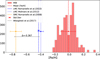 |
Fig. 9 Different metallicities found in the literature for MW Cepheids (red), LMC (blue), and SMC (orange; see Sect. 7 for details). |
8 Results
8.1 Period–Wesenheit relations in the Gaia passbands
The first aim of this approach is to be as independent as possible of the extinction (especially for the MW Cepheids). We considered that the Cepheids in the three clouds should follow the PW relation. Those that did not follow the relation might be stars with an incorrectly determined magnitude and undetected or incorrectly classified companions (DCEP and FUNDAMENTAL in Gaia). We derived the extinction-free absolute Wesenheit magnitude using the following equation (Ripepi et al. 2019):
![Mathematical equation: $\[\mathrm{W}_{\mathrm{G}}=\left(\mathrm{G}-5 ~\log _{10}(\mathrm{~d})+5\right)-1.90\left(\mathrm{G}_{\mathrm{BP}}-\mathrm{G}_{\mathrm{RP}}\right),\]$](/articles/aa/full_html/2026/02/aa57995-25/aa57995-25-eq37.png) (10)
(10)
where G is the apparent magnitude, d is the distance in parsec, and (GBP − GRP) is the colour index. In this section, all fitting procedure were made taking the barycenter of the measurement and the uncertainties on the y-axis into account (see Sect. 3.1 for details). We arbitrary rejected all stars above 1.75 times the RMS of the relation in order to retain most of the data (≈92%) while removing outliers. We tested clipping thresholds from 2.5σ to 1.5σ, and the resulting slopes and intercepts were all consistent within the uncertainties with our adopted value of 1.75σ. Fig. 10 (top) shows the three PW relations and the rejected stars for each galaxy corresponding to these relations
![Mathematical equation: $\[\mathrm{W}_{\mathrm{MW}}=-3.3090_{ \pm 0.0242} ~\log _{10}(\mathrm{P})-2.6595_{ \pm 0.0199}\]$](/articles/aa/full_html/2026/02/aa57995-25/aa57995-25-eq38.png) (11)
(11)
![Mathematical equation: $\[\mathrm{W}_{\mathrm{LMC}}=-3.3185_{ \pm 0.0049} ~\log _{10}(\mathrm{P})-2.4910_{ \pm 0.0033}\]$](/articles/aa/full_html/2026/02/aa57995-25/aa57995-25-eq39.png) (12)
(12)
![Mathematical equation: $\[\mathrm{W}_{\text {SMC }}=-3.4426_{ \pm 0.0062} ~\log _{10}(\mathrm{P})-2.3168_{ \pm 0.0034}.\]$](/articles/aa/full_html/2026/02/aa57995-25/aa57995-25-eq40.png) (13)
(13)
Eq. (11) is compatible with the result of Ripepi et al. (2019) for fundamental MW Cepheids. We plot in Figure 11 (a) the slopes and (b) the zero points of the three relations above as a function of the metallicity values described in Sect. 7. The slope appears to be independent of metallicity. In contrast, we observe a linear deviation between the zero points (ZP) and metallicities, which allowed us to adjust the relation between the zero points and average metallicities of the three galaxies (indicated in the plot),
![Mathematical equation: $\[\mathrm{ZP}_{\mathrm{PW}}=-0.5289_{ \pm 0.0136}[\mathrm{Fe} / \mathrm{H}]-2.7153_{ \pm 0.0082}.\]$](/articles/aa/full_html/2026/02/aa57995-25/aa57995-25-eq41.png) (14)
(14)
Ripepi et al. (2019) showed that the metallicity affects the slope of the PW relation in the Gaia bands only little, which agrees with several previous studies (Fiorentino et al. 2013; Ngeow et al. 2012; Di Criscienzo et al. 2013; Gieren et al. 2018). More recently, Ripepi et al. (2022) derived a new period–Wesenheit–metallicity relation in the Gaia bands and obtained a metallicity coefficient of c = −0.520±0.090, which directly affects the zero point of the PW relation. We determined the relation between the zero point and metallicity (see Eq. (14)). By rewriting this equation, W = a log10(P) − 2.7153±0.0082 − 0.5289±0.0136[Fe/H], with a that depends on the considered galaxies, the metallicity term we derive, −0.5289±0.0136, is fully consistent with the value derived by Ripepi et al. (2022) and with the constant term of the relations.
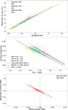 |
Fig. 10 Top: absolute period–Wesenheit (PW) relations for DCEP and FUNDAMENTAL MW, LMC, and SMC Cepheids. Middle: SBCRs using the Gaia GBP and GRP bands. The colour range is indicated in the legend. Bottom: relation between the PW fit residual and the SBCR residual relative to the calibrated SBCR represented by the dotted black line in the middle panel (only for MW Cepheids). |
8.2 Deriving the SBCRs in the MW, LMC, and SMC
After selecting the data based on quality criteria (Sect. 2), we determined the distances of each Cepheid (Sect. 4), corrected the magnitudes for the extinction (Sect. 6), and finally, rejected stars that did not follow the PW relations (Sect. 8.1). Finally, we derived the average angular diameter of each star using Eq. (5) and the PR relation we derived (Eq. (2)), which allowed us to obtain the surface brightness using Eq. (6) and the colour of each star. Fitting the three relations, we found
![Mathematical equation: $\[\mathrm{F}_{\mathrm{G}_{\mathrm{BP}}, \mathrm{MW}}=-0.2940_{ \pm 0.0175}\left(\mathrm{G}_{\mathrm{BP}}-\mathrm{G}_{\mathrm{RP}}\right)_0+3.9870_{ \pm 0.0151}\]$](/articles/aa/full_html/2026/02/aa57995-25/aa57995-25-eq42.png) (15)
(15)
![Mathematical equation: $\[\mathrm{F}_{\mathrm{G}_{\mathrm{BP}}, \mathrm{LMC}}=-0.2644_{ \pm 0.0070}\left(\mathrm{G}_{\mathrm{BP}}-\mathrm{G}_{\mathrm{RP}}\right)_0+3.9433_{ \pm 0.0053}\]$](/articles/aa/full_html/2026/02/aa57995-25/aa57995-25-eq43.png) (16)
(16)
![Mathematical equation: $\[\mathrm{F}_{\mathrm{G}_{\mathrm{BP}}, \mathrm{SMC}}=-0.2450_{ \pm 0.0083}\left(\mathrm{G}_{\mathrm{BP}}-\mathrm{G}_{\mathrm{RP}}\right)_0+3.9188_{ \pm 0.0058},\]$](/articles/aa/full_html/2026/02/aa57995-25/aa57995-25-eq44.png) (17)
(17)
with an RMS of 0.0223, 0.0096, and 0.0149 respectively. The colour range is indicated in the middle panel of Fig. 10. In Fig. 10, we overplot the latest SBCR for MW Cepheids calibrated by Bailleul et al. (2025) by interferometry (dashed black line). First, the SBCR (MW) derived here agrees well with the previous calibrated one (Bailleul et al. 2025) based on direct interferometric measurements. The SBCR (MW) calibrated by interferometry remains the one that should be used in forthcoming studies. Secondly, the SBCR (LMC) agrees well with the theoretical SBCR for metal-poor Cepheids derived by Bailleul et al. (2025) (see the middle panel of Fig. 10). Thirdly, we observe that the zero point (as expected) and also the slope of the SBCR are affected by the metallicity. In Figure 11 we plot (c) the slopes and (d) the zero points of the three SBCRs as a function of the metallicity. We clearly observe a linear relation between these quantities. We also show the SBCR calibrated by Bailleul et al. (2025) (black dots). In addition, we fitted a linear relation between the slopes, the zero points, and the metallicity using the result of this work (dotted line) and the calibrated SBCR (purple line),
![Mathematical equation: $\[\text {Slope}_{\text {SBCR}}=-0.0777_{ \pm 0.0106}[\mathrm{Fe} / \mathrm{H}]-0.3009_{ \pm 0.0030}\]$](/articles/aa/full_html/2026/02/aa57995-25/aa57995-25-eq45.png) (18)
(18)
![Mathematical equation: $\[\mathrm{ZP}_{\mathrm{SBCR}}=0.1121_{ \pm 0.0082}[\mathrm{Fe} / \mathrm{H}]+3.9983_{ \pm 0.0029}.\]$](/articles/aa/full_html/2026/02/aa57995-25/aa57995-25-eq46.png) (19)
(19)
The fit was performed without taking the barycenter of the measurement into account. This result shows that the use of a Gaia SBCR, calibrated for stars with solar metallicity, cannot be applied to stars with different metallicities without running the risk of determining the angular diameter incorrectly. Fourth, we observed and validated the fact that there is a direct link between the residual of the PW(MW) relation and the residual relative to the calibrated SBCR of the SBCR (MW). This indicates that physically, Cepheids that do not correctly follow the PW relation not correctly follow the SBCR either (see Fig. 10, lower panel). Finally, we derived the SBCRs associated with all the PR relation presented in Table 1. The resulting slopes and zero points are plotted in Fig. 12. Again, we find some correlation between the slope and zero point, as in Fig. 4 for the PR relations. As described above, however, the trend in Fig. 4 arises because the different authors did not fit their data taking the barycenters of the measurements into account in x and y, respectively which generates a larger correlation between the fitted slope and the zero point of their relation. Although this trend is observed in PR relations (Fig. 4), there is no clear effect of the metallicity, however. Conversely, in Fig. 12, we clearly find three different groups of SBCRs (slope and zero point) for the MW, LMC, and SMC. These results show that the metallicity significantly affects the SBCR, while its effect on PR relations is negligible or even null. Metallic lines are numerous in the large wavelength domain of Gaia, which significantly increases the corresponding magnitudes, while the radius derived either from interferometry or SBCR (V, V-K) is known to be weakly affected by the metallicity.
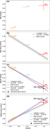 |
Fig. 11 Panels a and b: slopes and zero points from Eqs. (11)–(13) as a function of [Fe/H]. We adopted the average [Fe/H] value in Sect. 7 for the MW and the values from Romaniello et al. (2008) and Romaniello et al. (2022) for the SMC and LMC, respectively. Panels c and d: same, but for the SBCRs from Eqs. (15)–(17). |
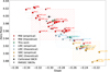 |
Fig. 12 Zero point and slope of the different SBCRs determined using the different PR relations in Table 1. We show the calibrated and theoretical (PARSEC) SBCRs for solar and metal poor Cepheids determined by Bailleul et al. (2025) (black). The turquoise points indicate the slope and zero point of the SBCRs (MW, LMC, and SMC) using the PR relation calibrated in this paper. In the centre of each dashed rectangle, the mean value is indicated with a black cross. The height (width) of the rectangle is three times the standard deviation (3σ) of the zero points found using the various PR relations. Relations without an uncertainty in Table 1 are shown without uncertainty in this figure. |
9 Conclusion
Bailleul et al. (2025) recently derived an SBCR for the first time based exclusively on Gaia photometric bands for fundamentalmode classical Cepheids of solar metallicity. This result is of particular interest because Gaia represents one of the largest available Cepheid databases. The authors also demonstrated theoretically that the Gaia-based SBCR is highly sensitive to metallicity. We confirmed these findings empirically for the first time by deriving SBCRs for Cepheids in the Milky Way, Large Magellanic Cloud, and Small Magellanic Cloud. We demonstrated and quantified the effect of metallicity on the slope and zero point of these relations. With this work, we aim to open a new avenue for the application of the inverse Baade–Wesselink method to Galactic and Magellanic Cloud Cepheids in the Gaia sample in order to investigate their physical properties, and in particular, their projection factor Nardetto et al. (2004, 2007). The current study is limited by the inhomogeneous and relatively small number of available metallicity measurements for Cepheids. The forthcoming Gaia Data Release 4 (DR4) is expected to dramatically improve this situation by providing epoch metallicities for a larger number of stars and with an improved precision, however. The overall goal of the Unlockpfactor project (Nardetto et al. 2023) is to shed light on the projection factor in order to pave the way for the application of the Baade–Wesselink method within the Local Group using ELT spectroscopic instruments, in particular, MOSAIC (Pelló et al. 2024) and ANDES (Marconi et al. 2024).
Acknowledgements
The authors acknowledge the support of the French Agence Nationale de la Recherche (ANR), under grant ANR-23-CE31-0009-01 (Unlockpfactor) and the financial support from “Programme National de Physique Stellaire” (PNPS) of CNRS/INSU, France. This research has made use of the SIMBAD and VIZIER (available at http://cdsweb.u-strasbg.fr/) databases at CDS, Strasbourg (France), and of the electronic bibliography maintained by the NASA/ADS system. This work has made use of data from the European Space Agency (ESA) mission Gaia (https://www.cosmos.esa.int/gaia), processed by the Gaia Data Processing and Analysis Consortium (DPAC, https://www.cosmos.esa.int/web/gaia/dpac/consortium). Funding for the DPAC has been provided by national institutions, in particular the institutions participating in the Gaia Multilateral Agreement. The research leading to these results has received funding from the European Research Council (ERC) under the European Union’s Horizon 2020 research and innovation program (projects CepBin, grant agreement 695099, and UniverScale, grant agreement 951549). This research has used data, tools or materials developed as part of the EXPLORE project that has received funding from the European Union’s Horizon 2020 research and innovation programme under grant agreement No 101004214. WG gratefully acknowledges financial support for this work from the BASAL Centro de Astrofisica y Tecnologias Afines (CATA) PFB-06/2007, and from the Millenium Institute of Astrophysics (MAS) of the Iniciativa Cientifica Milenio del Ministerio de Economia, Fomento y Turismo de Chile, project IC120009. WG also acknowledges support from the ANID BASAL project ACE210002. Support from the Polish National Science Center grant MAESTRO 2012/06/A/ST9/00269 and 2024/WK/02 grants of the Polish Minstry of Science and Higher Education is also acknowledged. AG acknowledges the support of the Agencia Nacional de Investigación Científica y Desarrollo (ANID) through the FONDECYT Regular grant 1241073. A.G. acknowledges support from the ANID-ALMA fund No. ASTRO20-0059. B.P. gratefully acknowledges support from the Polish National Science Center grant SONATA BIS 2020/38/E/ST9/00486. This research has been supported by the Polish–French Marie Skłodowska–Curie and Pierre Curie Science Prize awarded by the Foundation for Polish Science.
References
- Alibert, Y., Baraffe, I., Hauschildt, P., & Allard, F. 1999, arXiv Version Number: 1 [Google Scholar]
- Asplund, M., Grevesse, N., Sauval, A. J., & Scott, P. 2009, ARA&A, 47, 481 [CrossRef] [Google Scholar]
- Bailer-Jones, C. A. L. 2023, AJ, 166, 269 [NASA ADS] [CrossRef] [Google Scholar]
- Bailer-Jones, C. A. L., Rybizki, J., Fouesneau, M., Demleitner, M., & Andrae, R. 2021, AJ, 161, 147 [Google Scholar]
- Bailleul, M. C., Nardetto, N., Hocdé, V., et al. 2025, Surface brightness–colour relations of Cepheids calibrated by optical interferometry [Google Scholar]
- Balona, L. A. 1977, MNRAS, 178, 231 [NASA ADS] [CrossRef] [Google Scholar]
- Barnes, T. G., & Evans, D. S. 1976, MNRAS, 174, 489 [Google Scholar]
- Benedict, G. F., McArthur, B. E., Fredrick, L. W., et al. 2002, AJ, 124, 1695 [NASA ADS] [CrossRef] [Google Scholar]
- Benedict, G. F., McArthur, B. E., Feast, M. W., et al. 2007, AJ, 133, 1810 [NASA ADS] [CrossRef] [Google Scholar]
- Bono, G., Caputo, F., & Marconi, M. 1998, ApJ, 497, L43 [Google Scholar]
- Breuval, L., Kervella, P., Wielgórski, P., et al. 2021, ApJ, 913, 38 [NASA ADS] [CrossRef] [Google Scholar]
- Caccin, R., Onnembo, A., Russo, G., & Sollazzo, C. 1981, A&A, 97, 104 [NASA ADS] [Google Scholar]
- Campante, T. L., Corsaro, E., Lund, M. N., et al. 2019, ApJ, 885, 31 [Google Scholar]
- Castelli, F., & Kurucz, R. L. 2003, in IAU Symposium, 210, Modelling of Stellar Atmospheres, eds. N. Piskunov, W. W. Weiss, & D. F. Gray, A20 [Google Scholar]
- Cogan, B. C. 1978, ApJ, 221, 635 [Google Scholar]
- De Somma, G., Marconi, M., Molinaro, R., et al. 2020, ApJS, 247, 30 [Google Scholar]
- De Somma, G., Marconi, M., Molinaro, R., et al. 2022, ApJS, 262, 25 [NASA ADS] [CrossRef] [Google Scholar]
- di Benedetto, G. P. 1994, A&A, 285, 819 [Google Scholar]
- Di Criscienzo, M., Marconi, M., Musella, I., Cignoni, M., & Ripepi, V. 2013, MNRAS, 428, 212 [NASA ADS] [CrossRef] [Google Scholar]
- Di Mauro, M. P., Reda, R., Mathur, S., et al. 2022, ApJ, 940, 93 [NASA ADS] [CrossRef] [Google Scholar]
- Di Valentino, E., Said, J. L., Riess, A., et al. 2025, Phys. Dark Universe, 49, 101965 [Google Scholar]
- Fernie, J. D. 1984, ApJ, 282, 641 [Google Scholar]
- Fiorentino, G., Musella, I., & Marconi, M. 2013, MNRAS, 434, 2866 [Google Scholar]
- Fouque, P., & Gieren, W. P. 1997, A&A, 320, 799 [NASA ADS] [Google Scholar]
- Gaia Collaboration (Prusti, T., et al.) 2016, A&A, 595, A1 [NASA ADS] [CrossRef] [EDP Sciences] [Google Scholar]
- Gaia Collaboration 2020, VizieR Online Data Catalog: Gaia EDR3 (Gaia Collaboration, 2020), VizieR On-line Data Catalog: I/350. Originally published in: 2021A&A...649A...1G [Google Scholar]
- Gaia Collaboration 2022, VizieR Online Data Catalog: Gaia DR3 Part 4. Variability (Gaia Collaboration, 2022), VizieR On-line Data Catalog: I/358. Originally published in: 2023A&A...674A...1G [Google Scholar]
- Gaia Collaboration (Montegriffo, P., et al.) 2023a, A&A, 674, A33 [CrossRef] [EDP Sciences] [Google Scholar]
- Gaia Collaboration (Vallenari, A., et al.) 2023b, A&A, 674, A1 [NASA ADS] [CrossRef] [EDP Sciences] [Google Scholar]
- Gallenne, A., Kervella, P., Mérand, A., et al. 2017, A&A, 608, A18 [NASA ADS] [CrossRef] [EDP Sciences] [Google Scholar]
- Genovali, K., Lemasle, B., Bono, G., et al. 2014, A&A, 566, A37 [NASA ADS] [CrossRef] [EDP Sciences] [Google Scholar]
- Genovali, K., Lemasle, B., da Silva, R., et al. 2015, A&A, 580, A17 [NASA ADS] [CrossRef] [EDP Sciences] [Google Scholar]
- Gent, M. R., Bergemann, M., Serenelli, A., et al. 2022, A&A, 658, A147 [NASA ADS] [CrossRef] [EDP Sciences] [Google Scholar]
- Gieren, W., Storm, J., Konorski, P., et al. 2018, A&A, 620, A99 [NASA ADS] [CrossRef] [EDP Sciences] [Google Scholar]
- Gieren, W. P., Moffett, T. J., & Barnes Iii, T. G. 1999, ApJ, 512, 553 [NASA ADS] [CrossRef] [Google Scholar]
- Górski, M., Zgirski, B., Pietrzyński, G., et al. 2020, ApJ, 889, 179 [Google Scholar]
- Graczyk, D., Pietrzyński, G., Thompson, I. B., et al. 2020, ApJ, 904, 13 [Google Scholar]
- Groenewegen, M. A. T. 2007, A&A, 474, 975 [NASA ADS] [CrossRef] [EDP Sciences] [Google Scholar]
- Groenewegen, M. A. T. 2013, A&A, 550, A70 [NASA ADS] [CrossRef] [EDP Sciences] [Google Scholar]
- Hocdé, V., Smolec, R., Moskalik, P., Ziółkowska, O., & Singh Rathour, R. 2023, A&A, 671, A157 [NASA ADS] [CrossRef] [EDP Sciences] [Google Scholar]
- Jacyszyn-Dobrzeniecka, A. M., Skowron, D. M., Mróz, P., et al. 2016, Acta Astron., 66, 149 [NASA ADS] [Google Scholar]
- Karp, A. H. 1975, ApJ, 199, 448 [Google Scholar]
- Kervella, P., Bersier, D., Mourard, D., Nardetto, N., & Coudé du Foresto, V. 2004a, A&A, 423, 327 [NASA ADS] [CrossRef] [EDP Sciences] [Google Scholar]
- Kervella, P., Fouqué, P., Storm, J., et al. 2004b, ApJ, 604, L113 [NASA ADS] [CrossRef] [Google Scholar]
- Kervella, P., Nardetto, N., Bersier, D., Mourard, D., & Coudé du Foresto, V. 2004c, A&A, 416, 941 [NASA ADS] [CrossRef] [EDP Sciences] [Google Scholar]
- Kervella, P., Bond, H. E., Cracraft, M., et al. 2014, A&A, 572, A7 [NASA ADS] [CrossRef] [EDP Sciences] [Google Scholar]
- Kovtyukh, V. V., Korotin, S. A., Andrievsky, S. M., Matsunaga, N., & Fukue, K. 2022, MNRAS, 516, 4269 [NASA ADS] [CrossRef] [Google Scholar]
- Lallement, R., Vergely, J. L., Babusiaux, C., & Cox, N. L. J. 2022, A&A, 661, A147 [NASA ADS] [CrossRef] [EDP Sciences] [Google Scholar]
- Lane, B. F., Creech-Eakman, M. J., & Nordgren, T. E. 2002, ApJ, 573, 330 [NASA ADS] [CrossRef] [Google Scholar]
- Laney, C. D., & Stobie, R. S. 1995, MNRAS, 274, 337 [NASA ADS] [Google Scholar]
- Lindegren, L., Klioner, S. A., Hernández, J., et al. 2021, A&A, 649, A2 [EDP Sciences] [Google Scholar]
- Lindemann, F. A. 1918, MNRAS, 78, 639 [NASA ADS] [CrossRef] [Google Scholar]
- Luck, R. E. 2018, AJ, 156, 171 [Google Scholar]
- Luck, R. E., Andrievsky, S. M., Kovtyukh, V. V., Gieren, W., & Graczyk, D. 2011, AJ, 142, 51 [NASA ADS] [CrossRef] [Google Scholar]
- Mamajek, E. E., Torres, G., Prsa, A., et al. 2015, arXiv e-prints [arXiv:1510.06262] [Google Scholar]
- Marconi, A., Abreu, M., Adibekyan, V., et al. 2024, SPIE Conf. Ser., 13096, 1309613 [Google Scholar]
- Mérand, A., Kervella, P., Breitfelder, J., et al. 2015, A&A, 584, A80 [NASA ADS] [CrossRef] [EDP Sciences] [Google Scholar]
- Moffett, T. J., & Barnes, Iii, T. J. 1987, ApJ, 323, 280 [Google Scholar]
- Molinaro, R., Ripepi, V., Marconi, M., et al. 2012a, Mem. Soc. Astron. Ital. Suppl., 19, 205 [NASA ADS] [Google Scholar]
- Molinaro, R., Ripepi, V., Marconi, M., et al. 2012b, ApJ, 748, 69 [NASA ADS] [CrossRef] [Google Scholar]
- Mucciarelli, A., Bellazzini, M., & Massari, D. 2021, A&A, 653, A90 [NASA ADS] [CrossRef] [EDP Sciences] [Google Scholar]
- Nardetto, N., Fokin, A., Mourard, D., et al. 2004, A&A, 428, 131 [CrossRef] [EDP Sciences] [Google Scholar]
- Nardetto, N., Mourard, D., Mathias, P., Fokin, A., & Gillet, D. 2007, A&A, 471, 661 [NASA ADS] [CrossRef] [EDP Sciences] [Google Scholar]
- Nardetto, N., Gieren, W., Storm, J., et al. 2023, A&A, 671, A14 [NASA ADS] [CrossRef] [EDP Sciences] [Google Scholar]
- Ngeow, C.-C., Kanbur, S. M., Bellinger, E. P., et al. 2012, Ap&SS, 341, 105 [Google Scholar]
- Pelló, R., Puech, M., Prieto, É., et al. 2024, SPIE Conf. Ser., 13096, 1309615 [Google Scholar]
- Perryman, M. A. C., Lindegren, L., Kovalevsky, J., et al. 1997, A&A, 323, L49 [Google Scholar]
- Petroni, S., Bono, G., Marconi, M., & Stellingwerf, R. 2003, ApJ, 599, 522 [CrossRef] [Google Scholar]
- Pietrzyński, G., Graczyk, D., Gieren, W., et al. 2013, Nature, 495, 76 [Google Scholar]
- Pietrzyński, G., Graczyk, D., Gallenne, A., et al. 2019, Nature, 567, 200 [Google Scholar]
- Pilecki, B., Gieren, W., Pietrzyński, G., et al. 2018, ApJ, 862, 43 [NASA ADS] [CrossRef] [Google Scholar]
- Riello, M., De Angeli, F., Evans, D. W., et al. 2021, A&A, 649, A3 [NASA ADS] [CrossRef] [EDP Sciences] [Google Scholar]
- Recio-Blanco, A., de Laverny, P., Palicio, P. A., et al. 2023, A&A, 674, A29 [NASA ADS] [CrossRef] [EDP Sciences] [Google Scholar]
- Riess, A. G., Yuan, W., Macri, L. M., et al. 2022, ApJ, 934, L7 [NASA ADS] [CrossRef] [Google Scholar]
- Riess, A. G., Scolnic, D., Anand, G. S., et al. 2024, ApJ, 977, 120 [NASA ADS] [CrossRef] [Google Scholar]
- Rimoldini, L., Eyer, L., Audard, M., et al. 2022, Gaia DR3 documentation Chapter 10: Variability [Google Scholar]
- Ripepi, V., Barone, F., Milano, L., & Russo, G. 1996, Cepheid Radii and the Cors Method Revisited, version Number: 1 [Google Scholar]
- Ripepi, V., Barone, F., Milano, L., & Russo, G. 1997, A&A, 318, 797 [NASA ADS] [Google Scholar]
- Ripepi, V., Molinaro, R., Musella, I., et al. 2019, A&A, 625, A14 [NASA ADS] [CrossRef] [EDP Sciences] [Google Scholar]
- Ripepi, V., Catanzaro, G., Molinaro, R., et al. 2021, MNRAS, 508, 4047 [NASA ADS] [CrossRef] [Google Scholar]
- Ripepi, V., Catanzaro, G., Clementini, G., et al. 2022, A&A, 659, A167 [NASA ADS] [CrossRef] [EDP Sciences] [Google Scholar]
- Rojo Arellano, E., & Arellano Ferro, A. 1994, Rev. Mex. Astron. Astrofis., 29, 148 [Google Scholar]
- Romaniello, M., Primas, F., Mottini, M., et al. 2008, A&A, 488, 731 [NASA ADS] [CrossRef] [EDP Sciences] [Google Scholar]
- Romaniello, M., Riess, A., Mancino, S., et al. 2022, A&A, 658, A29 [NASA ADS] [CrossRef] [EDP Sciences] [Google Scholar]
- Ruoppo, A., Ripepi, V., Marconi, M., & Russo, G. 2004, A&A, 422, 253 [NASA ADS] [CrossRef] [EDP Sciences] [Google Scholar]
- Salsi, A., Nardetto, N., Plez, B., & Mourard, D. 2022, A&A, 662, A120 [NASA ADS] [CrossRef] [EDP Sciences] [Google Scholar]
- Skowron, D. M., Skowron, J., Mróz, P., et al. 2019, Science, 365, 478 [Google Scholar]
- Sollazzo, C., Russo, G., Onnembo, A., & Caccin, B. 1981, A&A, 99, 66 [Google Scholar]
- Storm, J., Gieren, W., Fouqué, P., et al. 2011, A&A, 534, A94 [CrossRef] [EDP Sciences] [Google Scholar]
- Trahin, B., Breuval, L., Kervella, P., et al. 2021, A&A, 656, A102 [NASA ADS] [CrossRef] [EDP Sciences] [Google Scholar]
- Trentin, E., Ripepi, V., Catanzaro, G., et al. 2023, MNRAS, 519, 2331 [Google Scholar]
- Turner, D. G., & Burke, J. F. 2002, AJ, 124, 2931 [NASA ADS] [CrossRef] [Google Scholar]
- Valle, G., Dell’Omodarme, M., Prada Moroni, P. G., & Degl’Innocenti, S. 2024, A&A, 690, A327 [NASA ADS] [CrossRef] [EDP Sciences] [Google Scholar]
- van Hoof, A. 1945, Ciel Terre, 61, 11 [Google Scholar]
- van Leeuwen, F. 2007, A&A, 474, 653 [CrossRef] [EDP Sciences] [Google Scholar]
- van Leeuwen, F., Feast, M. W., Whitelock, P. A., & Laney, C. D. 2007, MNRAS, 379, 723 [NASA ADS] [CrossRef] [Google Scholar]
- Vergely, J. L., Lallement, R., & Cox, N. L. J. 2022, A&A, 664, A174 [NASA ADS] [CrossRef] [EDP Sciences] [Google Scholar]
- Wang, S., & Chen, X. 2023, ApJ, 946, 43 [Google Scholar]
- Wesselink, A. J. 1969, MNRAS, 144, 297 [NASA ADS] [CrossRef] [Google Scholar]
- Wielgórski, P., Pietrzyński, G., Gieren, W., et al. 2017, ApJ, 842, 116 [CrossRef] [Google Scholar]
All Tables
All Figures
|
Fig. 1 Data selection process. |
| In the text | |
|
Fig. 2 Gaia all-sky view of the Milky Way and the Large and Small Magellanic Clouds. We show the total sample in grey. The final selected sample of Cepheids is shown in colour. |
| In the text | |
|
Fig. 3 Period-radius relation using data of seven Cepheids based on the interferometric angular diameter curve of Bailleul et al. (2025). |
| In the text | |
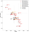 |
Fig. 4 Slope and zero points of the different period–radius relations listed in Table 1. |
| In the text | |
|
Fig. 5 Gaia zero-point offset as a function of the distance difference that it implies. The colour represents the parallax. Only the 228 selected Cepheids (after the whole selection process shown in Fig. 1) are shown here. |
| In the text | |
|
Fig. 6 LMC and SMC Cepheids within 3 and 0.6 degrees, respectively, from the clouds centre. |
| In the text | |
|
Fig. 7 HR diagram for MW Cepheids and position of the red and blue edge of the theoretical IS for Z=0.03 (dashed line) and Z=0.008 (dotted line). |
| In the text | |
|
Fig. 8 LMC (left) and SMC (right) extinction maps (RA vs. Dec) from Górski et al. (2020) with matched Cepheids from our sample. The colour map indicates the value of E(B − V) at a certain location. |
| In the text | |
|
Fig. 9 Different metallicities found in the literature for MW Cepheids (red), LMC (blue), and SMC (orange; see Sect. 7 for details). |
| In the text | |
|
Fig. 10 Top: absolute period–Wesenheit (PW) relations for DCEP and FUNDAMENTAL MW, LMC, and SMC Cepheids. Middle: SBCRs using the Gaia GBP and GRP bands. The colour range is indicated in the legend. Bottom: relation between the PW fit residual and the SBCR residual relative to the calibrated SBCR represented by the dotted black line in the middle panel (only for MW Cepheids). |
| In the text | |
|
Fig. 11 Panels a and b: slopes and zero points from Eqs. (11)–(13) as a function of [Fe/H]. We adopted the average [Fe/H] value in Sect. 7 for the MW and the values from Romaniello et al. (2008) and Romaniello et al. (2022) for the SMC and LMC, respectively. Panels c and d: same, but for the SBCRs from Eqs. (15)–(17). |
| In the text | |
|
Fig. 12 Zero point and slope of the different SBCRs determined using the different PR relations in Table 1. We show the calibrated and theoretical (PARSEC) SBCRs for solar and metal poor Cepheids determined by Bailleul et al. (2025) (black). The turquoise points indicate the slope and zero point of the SBCRs (MW, LMC, and SMC) using the PR relation calibrated in this paper. In the centre of each dashed rectangle, the mean value is indicated with a black cross. The height (width) of the rectangle is three times the standard deviation (3σ) of the zero points found using the various PR relations. Relations without an uncertainty in Table 1 are shown without uncertainty in this figure. |
| In the text | |
Current usage metrics show cumulative count of Article Views (full-text article views including HTML views, PDF and ePub downloads, according to the available data) and Abstracts Views on Vision4Press platform.
Data correspond to usage on the plateform after 2015. The current usage metrics is available 48-96 hours after online publication and is updated daily on week days.
Initial download of the metrics may take a while.