| Issue |
A&A
Volume 706, February 2026
|
|
|---|---|---|
| Article Number | L12 | |
| Number of page(s) | 6 | |
| Section | Letters to the Editor | |
| DOI | https://doi.org/10.1051/0004-6361/202558370 | |
| Published online | 10 February 2026 | |
Letter to the Editor
Time delays for the quadruply lensed QSO GraL J1651-0417 based on ZTF light curves
1
Instituto de Física y Astronomía, Universidad de Valparaíso Gran Bretaña 1111 Valparaíso, Chile
2
Millennium Nucleus on Transversal Research and Technology to Explore Supermassive Black Holes (TITANS) Valparaíso, Chile
3
Millennium Institute of Astrophysics (MAS) Nuncio Monseñor Sótero Sanz 100 Providencia Santiago, Chile
★ Corresponding author: This email address is being protected from spambots. You need JavaScript enabled to view it.
Received:
3
December
2025
Accepted:
13
January
2026
Abstract
Aims We aim to test the possibility of measuring significant and accurate time delays between images of lensed quasars using public photometric surveys. We show the case for the large-separation, quadruply lensed quasi-stellar object (QSO) GraL J1651-0417.
Methods We retrieved publicly available light curves in the g and r bands from the ZTF forced photometry service centred on the four images of the quasar. We estimated the time delays of the flux variations in the different images using the discrete correlation function and bootstrapping methods separately for each band. The delays were independently predicted by fitting two mass lens model (SIS+γ and SPL+γ).
Results The ZTF light curves reveal significant correlations and time delays. In the r band, we measure delays of 579 ± 40 days for A-B, 366 ± 26 days for A-C, and 698 ± 29 days for A-D, which are fully consistent with the predictions from the lens model.
Key words: gravitational lensing: strong / quasars: general / quasars: individual: GraL J1651-0417
© The Authors 2026
 Open Access article, published by EDP Sciences, under the terms of the Creative Commons Attribution License (https://creativecommons.org/licenses/by/4.0), which permits unrestricted use, distribution, and reproduction in any medium, provided the original work is properly cited.
This article is published in open access under the Subscribe to Open model. This email address is being protected from spambots. You need JavaScript enabled to view it. to support open access publication.
1. Introduction
The strong gravitational lensing of quasars produces multiple images of the same source, separated by angular scales of the order of arcseconds. Due to the different paths that light takes to reach the observer, a time delay occurs between the formed images. Measurement of these time delays provides an independent method for determining the value of the Hubble constant (H0; Refsdal 1964; Saha et al. 2006; Oguri 2007; Bonvin et al. 2017; Wong et al. 2020; Birrer et al. 2024; TDCOSMO Collaboration 2025), as well as for studying the mass distribution of the lens (Mohammed et al. 2015; Rusin 2000; Vegetti et al. 2024; Shajib et al. 2024).
In this context, quadruple-imaged quasars are especially valuable because four images allow for multiple independent time-delay measurements. This type of system is difficult to find, making each new measure an important contribution to the field. GraL J1651-0417, nicknamed the ‘Dragon Kite’ (see Fig. 1), is a recently discovered quadruple lensed quasar identified by the Gaia Gravitational Lenses (GraL) collaboration (Stern et al. 2021, hereafter, Stern21). It exhibits a maximum image separation of ≃10″ (i.e. that of the pair most widely separated in its sample), with a source redshift of zs ≃ 1.451 and a deflector redshift of zl = 0.591. So far, no precise time-delay values have been published for this system.
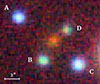 |
Fig. 1. Red-green-blue composite image of the Dragon Kite created from Pan-STARRS g, i, and y bands. North is up, and east is to the left. |
We present the first estimation of the time delays in the Dragon Kite, based on the Zwicky Transient Facility (ZTF; Bellm et al. 2019; Masci et al. 2019) g- and r-band light curves spanning seven years. Although ZTF light curves are not specifically designed for time-delay measurements, their cadence and temporal coverage allow us to perform such an analysis. Moreover, dedicated monitoring campaigns capable of measuring time delays, particularly those requiring multi-year coverage, are observationally expensive, which makes the use of publicly available ZTF data a valuable and efficient alternative for extending time-delay studies.
In this study we determined the delays between image pairs in the ZTF light curves using the discrete correlation function, and then compared our results with two gravitational lens models. The agreement between our delay estimates and model predictions confirms that our approach is robust. This result demonstrates the potential of large, public photometric surveys to constrain widely separated, and therefore also long-delay, lensed systems.
2. Data and estimation of time delays
The ZTF is a wide-field time-domain survey conducted using the 48-inch Samuel Oschin Telescope to monitor the northern sky in the g, r, and i bands with high cadence (∼3-night cadence; Bellm et al. 2019). Since 2018, ZTF has repeatedly observed millions of variable sources, providing light curves that are publicly available through data releases and a forced photometry service.
We used the forced photometry service to obtain a light curve at the position of each image presented in Stern21. The resulting ZTF magnitudes were calibrated to the Pan-STARRS photometric system by applying colour-term corrections. For image C in the r band, we applied a flux correction ΔF = 0.6 × 10⁻⁸ to the forced photometry fluxes before converting to magnitudes to compensate for an incorrectly assigned (nearby brighter) source in the reference image. This source is located to the right of image C in Fig. 1, and the applied correction corresponds to approximately 30% of the measured flux of image C.
2.1. Discrete correlation function and magnitude offset
We used image A as the reference for all time-delay measurements (except for B; see Sect. 2.2). As a first approximation, we computed the discrete correlation function (DCF) described by Edelson & Krolik (1988) between the light curve of image A and each of the other light curves. To determine the range of delays with significant cross-correlations, we followed the procedure described in Arévalo et al. (2008). We created uncorrelated, simulated light curves with the same time sampling as one of the real light curves and calculated the DCF between this simulated light curve and the other, real light curve. The median and 95 and 99 percentiles of the resulting, uncorrelated, DCF values are plotted in the upper panels of Fig. 2 as a function of the time delay, τ, along with the DCF of the real data. We note that for each pair of light curves, there is a peak in the real DCF that surpasses over 99% of the uncorrelated DCFs. We therefore considered only these peaks as regions of significant correlation and continued to constrain its centroid with a bootstrap resampling procedure based on the flux randomization (FR) method of Peterson et al. (1998). We randomly selected 67% of the points in each light curve, calculated the DCF of each pair of real light curves, searched for its maximum value within the grey ranges marked in Fig. 2 (for the r band), and calculated the weighted mean of τ by integrating the DCF peak from its maximum to 50% of this value to either side; we repeated this process 1000 times. The mean and RMS of the resulting centroids are listed in Table 1 and represent the estimated delays and their errors for each pair of images and for each photometric filter. The corresponding DCFs and time lag histograms for the g band are consistent with those of the r band and are shown in Fig. A.1.
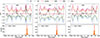 |
Fig. 2. Upper panels: DCF between each pair of images, in the r band. The red line represents the mean correlation of unrelated quasars (from simulations). The solid curves represent the percentiles of that distribution: fuchsia (99), orange (95), green (5), and light blue (1). These curves define the range of correlations expected from random, unrelated light curves. The dashed line is the actual cross-correlation between a real pair of light curves; it approaches the upper percentile around a specific time delay, indicating a significant correlation that is unlikely to happen by chance. Lower panels: Distribution of centroid positions obtained from the bootstrap resampling, reflecting the uncertainty on the centroid determination. |
Time delays in days.
To quantify the relative magnitude offset between images, we used their overlapping light curves after applying the measured time delays. For each pair of images, we linearly interpolated one light curve onto the time sampling of the other. The point-by-point magnitude difference was then computed as
 (1)
(1)
where m2(ti) is the interpolated magnitude of the second image at time ti and m1(ti) is the measured magnitude of the first image.
The associated uncertainty of each point was obtained by adding the individual photometric errors in quadrature,
 (2)
(2)
We then estimated the global magnitude offset as the weighted mean of the individual differences computed in Eq. (1).
The magnitude differences between the images are shown in Table 2. We note that these Δm are different in the g and r bands, which indicates differences in colour. In Table 3 we show the median g − r colours for each image, calculated from the mean magnitude of each ZTF light curve. The colours become consistently redder (i.e. larger) for images closer to the lens galaxy, suggesting a reddening by the lens. Alternatively, the difference in colour could be produced by chromatic microlensing.
Magnitude offsets between pairs of QSO images.
Magnitudes and colours of the QSO images.
In Fig. 3, we show both the original light curves and the light curves after applying the estimated delays and the magnitude offset. Figure A.2 shows the same procedure applied to the g-band light curves, with very similar results.
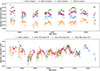 |
Fig. 3. Light curves from ZTF for each image in the r band. Upper panel: Observed light curves without any shift in magnitude or time. Lower panel: Same light curves shifted according to the time-delay and flux-ratio values derived in this work. |
2.2. Time delay for image B
The ZTF observing strategy introduces gaps in the light curves due to its windowed sampling. After applying the measured time delays to all images, the data of image B coincide with the gaps in images A, C, and D. To obtain a more robust estimate of the time delay for image B, we constructed a composite light curve from images A, C, and D. We note that the peak is more significant in the DCF (see Fig. A.4), with a time delay of 522 ± 52 days.
3. Lens model
We used two spherical mass distributions implemented in Lensmodel/Gravlens (Keeton 2001, 2011) to reproduce the four images: an isothermal sphere (SIS) and a softened power law (SPL; Blandford & Kochanek 1987), both with an external perturbation introduced by the shear (γ).
The free parameters for the SIS+γ are the lens position (ralens, declens), the Einstein radius (θE), and the shear and its position angle (θγ). For the case of SPL+γ, the free parameters are the same with the addition of the profile slope (α; for the SIS profile α = 1). Following the analysis of Stern21, we used as observables the astrometric positions of the images relative to the lens galaxy, along with the lens and source redshifts. As flux ratios can be affected by microlensing, we decided not to use them in the models.
The best-fitting parameters for this SIS+γ model are θE = 3.46 arcsec, ralens = 7 × 10⁻², declens = −5 × 10⁻², and γ = 0.32, θγ = 38.56, in good agreement with those obtained by Stern21. The resulting lag values are listed in Table 4. We note that the inferred external shear is relatively large (γ > 0.2), which may reflect contributions from nearby mass structures1. The large shear is also confirmed by the velocity dispersion estimated from θE (Grillo et al. 2008; Treu 2010), ∼ 495 km s−1, which is greater than the ∼ 300 km s−1 typically expected for an isolated elliptical galaxy. The best-fitting parameters for the SPL+γ are θE = 3.5 arcsec, ralens = 8.4 × 10⁻², declens = −1.8 × 10⁻², γ = 0.18, θγ = 38.56, and α = 1.44. We note that θE and the shear angle are in good agreement with the previous model. Notice that part of the shear strength has been absorbed by the slope (α). The resulting delays are also listed in Table 4. We note that both models produce time delays of the same approximate length and image arrival order as those measured from the light curves (copied in the last column of Table 4), with one model under-predicting and the other model over-predicting the measured delays. This difference is a consequence of the different gravitational potentials at the position of the images (Shajib et al. 2024).
Predicted and measured time delays (Δt).
The main limitation of these simple models is that they may provide an incomplete description of the lens environment. Nearby galaxies or group-scale structures along the line of sight can introduce additional deflections that are not fully captured by a single external shear term (Kochanek et al. 2000; Kochanek 2006; Fohlmeister et al. 2007). Neglecting such mass components may also affect the inferred Shapiro delay (Shapiro 1964). The presence of a group or cluster, or alternatively the ellipticity of the lens, will have to be constrained with deeper imaging and larger spectroscopic coverage, which are not currently available.
4. Conclusions
From the analysis of this work using ZTF forced photometry light curves of a known, wide-separation quadruply lensed QSO, we can conclude the following:
-
The public ZTF light curves can be effectively used to identify fluctuations exhibiting significant correlations. ZTF is one of the few campaigns capable of measuring such long time delays, thanks to its extensive multi-year observations.
-
The independently measured time delays from the g- and r-band light curves yield consistent values within their uncertainties.
-
The time delays measured exclusively from the light curves fall within the range predicted by both the SIS+γ and SPL+γ models, indicating overall consistency between the light curves and the lens modelling based on the astrometry.
-
The differences between the two models, together with the significant inferred velocity dispersion, indicate that the lens galaxy is embedded in a more massive environment. This reinforces the need for additional constraints beyond astrometry to accurately model the mass distribution.
-
Furthermore, the light curves provide the flux ratios between the lensed images, corrected for the measured time delays, which can further constrain the lens models. They also allowed us to determine the colours of the images at matched intrinsic variability phases, revealing a progressively redder colour for images closer to the lensing galaxy.
These results demonstrate the potential of large-area time-domain surveys such as ZTF for the characterization of lensed quasars using photometric data only. With the time delays of GraL J1651-0417 now measured, this system becomes a candidate for time-delay cosmography, particularly in the Vera Rubin LSST era, which should reduce the uncertainties in the time lags. However, the present measurements alone are not sufficient to derive a competitive constraint on H0. This would require high-resolution imaging to constrain the lens mass distribution and stellar kinematics of the main deflector, which could then be used to break degeneracies in the mass model and provide a detailed characterization of the lens environment.
Acknowledgments
We thank the anonymous referee for the useful comments that improve this letter. We acknowledge the Millennium Science Initiative Programs NCN2023_002 (CNP, PA) and AIM23-0001 (CNP, PA, VM), FONDECYT Regular 1241422 (PA), FONDECYT Regular 1231418 (VM, FAV), and CAV, CIDI N. 21 U. de Valparaíso, Chile (PA, VM). CNP and FAV thanks the Doctorate Fellowship program FIB-UV of the U. de Valparaíso for funding. Based on observations obtained with the Samuel Oschin Telescope 48-inch and the 60-inch Telescope at the Palomar Observatory as part of the Zwicky Transient Facility project. ZTF is supported by the National Science Foundation under Grants No. AST-1440341 and AST-2034437 and a collaboration including current partners Caltech, IPAC, the Weizmann Institute for Science, the Oskar Klein Center at Stockholm University, the University of Maryland, Deutsches Elektronen-Synchrotron and Humboldt University, the TANGO Consortium of Taiwan, the University of Wisconsin at Milwaukee, Trinity College Dublin, Lawrence Livermore National Laboratories, IN2P3, University of Warwick, Ruhr University Bochum, Northwestern University and former partners the University of Washington, Los Alamos National Laboratories, and Lawrence Berkeley National Laboratories. Operations are conducted by COO, IPAC, and UW.
References
- Arévalo, P., Uttley, P., Kaspi, S., et al. 2008, MNRAS, 389, 1479 [CrossRef] [Google Scholar]
- Bellm, E. C., Kulkarni, S. R., Graham, M. J., et al. 2019, PASP, 131, 018002 [Google Scholar]
- Birrer, S., Millon, M., Sluse, D., et al. 2024, Space Sci. Rev., 220, 48 [NASA ADS] [CrossRef] [Google Scholar]
- Blandford, R. D., & Kochanek, C. S. 1987, ApJ, 321, 658 [Google Scholar]
- Bonvin, V., Courbin, F., Suyu, S. H., et al. 2017, MNRAS, 465, 4914 [NASA ADS] [CrossRef] [Google Scholar]
- Edelson, R. A., & Krolik, J. H. 1988, ApJ, 333, 646 [Google Scholar]
- Fohlmeister, J., Kochanek, C. S., Falco, E. E., et al. 2007, ApJ, 662, 62 [NASA ADS] [CrossRef] [Google Scholar]
- Grillo, C., Lombardi, M., & Bertin, G. 2008, A&A, 477, 397 [NASA ADS] [CrossRef] [EDP Sciences] [Google Scholar]
- Keeton, C. R. 2001, arXiv e-prints [arXiv:astro-ph/0102340] [Google Scholar]
- Keeton, C. R. 2011, GRAVLENS: Computational Methods for Gravitational Lensing, Astrophysics Source Code Library [record ascl:1102.003] [Google Scholar]
- Kochanek, C. S. 2006, in Saas-Fee Advanced Course 33: Gravitational Lensing: Strong, Weak and Micro, eds. G. Meylan, P. Jetzer, P. North, et al. 91 [Google Scholar]
- Kochanek, C. S., Falco, E. E., Impey, C. D., et al. 2000, ApJ, 543, 131 [NASA ADS] [CrossRef] [Google Scholar]
- Masci, F. J., Laher, R. R., Rusholme, B., et al. 2019, PASP, 131, 018003 [Google Scholar]
- Mohammed, I., Saha, P., & Liesenborgs, J. 2015, PASJ, 67, 21 [NASA ADS] [CrossRef] [Google Scholar]
- Oguri, M. 2007, ApJ, 660, 1 [NASA ADS] [CrossRef] [Google Scholar]
- Peterson, B. M., Wanders, I., Horne, K., et al. 1998, PASP, 110, 660 [Google Scholar]
- Refsdal, S. 1964, MNRAS, 128, 307 [NASA ADS] [CrossRef] [Google Scholar]
- Rusin, D. 2000, arXiv e-prints [arXiv:astro-ph/0004241] [Google Scholar]
- Saha, P., Coles, J., Macciò, A. V., & Williams, L. L. R. 2006, ApJ, 650, L17 [NASA ADS] [CrossRef] [Google Scholar]
- Shajib, A. J., Vernardos, G., Collett, T. E., et al. 2024, Space Sci. Rev., 220, 87 [CrossRef] [Google Scholar]
- Shapiro, I. I. 1964, Phys. Rev. Lett., 13, 789 [Google Scholar]
- Stern, D., Djorgovski, S. G., Krone-Martins, A., et al. 2021, ApJ, 921, 42 [NASA ADS] [CrossRef] [Google Scholar]
- TDCOSMO Collaboration (Birrer, S., et al.) 2025, A&A, 704, A63 [Google Scholar]
- Treu, T. 2010, ARA&A, 48, 87 [NASA ADS] [CrossRef] [Google Scholar]
- Vegetti, S., Birrer, S., Despali, G., et al. 2024, Space Sci. Rev., 220, 58 [CrossRef] [Google Scholar]
- Wong, K. C., Suyu, S. H., Chen, G. C. F., et al. 2020, MNRAS, 498, 1420 [Google Scholar]
If instead the deflector is modelled as a singular isothermal ellipsoid, a comparable fit can be obtained with the ellipticity oriented along the same position angle, illustrating the well-known degeneracy between external shear and lens ellipticity in parametric lens models.
Appendix A: Supplementary material
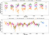 |
Fig. A.2. Same as Fig. 3 but using light curves in the g band and the shifts calculated for this band. |
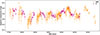 |
Fig. A.3. Light curves for ACD (i.e. the sum of epochs of images A, C, and D; in orange) and the light curve of image B (in fuchsia) in the r band. |
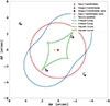 |
Fig. A.5. Schematics for SIS+γ, the best-fitting model when only the positions of the lens and the QSO images are considered for the χ2 minimization. |
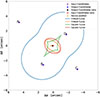 |
Fig. A.6. Schematics for SPL+γ, the best-fitting model when only the positions of the lens and QSO images are considered for the χ2 minimization. |
All Tables
All Figures
|
Fig. 1. Red-green-blue composite image of the Dragon Kite created from Pan-STARRS g, i, and y bands. North is up, and east is to the left. |
| In the text | |
|
Fig. 2. Upper panels: DCF between each pair of images, in the r band. The red line represents the mean correlation of unrelated quasars (from simulations). The solid curves represent the percentiles of that distribution: fuchsia (99), orange (95), green (5), and light blue (1). These curves define the range of correlations expected from random, unrelated light curves. The dashed line is the actual cross-correlation between a real pair of light curves; it approaches the upper percentile around a specific time delay, indicating a significant correlation that is unlikely to happen by chance. Lower panels: Distribution of centroid positions obtained from the bootstrap resampling, reflecting the uncertainty on the centroid determination. |
| In the text | |
|
Fig. 3. Light curves from ZTF for each image in the r band. Upper panel: Observed light curves without any shift in magnitude or time. Lower panel: Same light curves shifted according to the time-delay and flux-ratio values derived in this work. |
| In the text | |
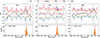 |
Fig. A.1. Same as Fig. 2 but using the light curves observed in the g band instead of the r band. |
| In the text | |
|
Fig. A.2. Same as Fig. 3 but using light curves in the g band and the shifts calculated for this band. |
| In the text | |
|
Fig. A.3. Light curves for ACD (i.e. the sum of epochs of images A, C, and D; in orange) and the light curve of image B (in fuchsia) in the r band. |
| In the text | |
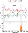 |
Fig. A.4. Same as Fig. 2 but for the DCF between image B and the composite light curve ACD. |
| In the text | |
|
Fig. A.5. Schematics for SIS+γ, the best-fitting model when only the positions of the lens and the QSO images are considered for the χ2 minimization. |
| In the text | |
|
Fig. A.6. Schematics for SPL+γ, the best-fitting model when only the positions of the lens and QSO images are considered for the χ2 minimization. |
| In the text | |
Current usage metrics show cumulative count of Article Views (full-text article views including HTML views, PDF and ePub downloads, according to the available data) and Abstracts Views on Vision4Press platform.
Data correspond to usage on the plateform after 2015. The current usage metrics is available 48-96 hours after online publication and is updated daily on week days.
Initial download of the metrics may take a while.