| Issue |
A&A
Volume 706, February 2026
|
|
|---|---|---|
| Article Number | L16 | |
| Number of page(s) | 4 | |
| Section | Letters to the Editor | |
| DOI | https://doi.org/10.1051/0004-6361/202558379 | |
| Published online | 18 February 2026 | |
Letter to the Editor
Juno’s high-spatial-resolution ultraviolet observations of Ganymede’s auroral patches
Constraints on the magnetospheric source region
1
Laboratory for Planetary and Atmospheric Physics, STAR Institute, University of Liège Liège, Belgium
2
Institute for Space Astrophysics and Planetology, National Institute for Astrophysics (INAF-IAPS) Rome, Italy
3
Institute of Geophysics and Meteorology, University of Cologne Cologne, Germany
4
Department of Earth & Planetary Sciences, University of Hong Kong Hong Kong, China
5
Aix-Marseille Université, CNRS, CNES, Institut Origines, LAM Marseille, France
6
Space Science Division, Southwest Research Institute San Antonio TX, USA
★ Corresponding author: This email address is being protected from spambots. You need JavaScript enabled to view it.
Received:
3
December
2025
Accepted:
20
January
2026
Abstract
Aims. We analyzed ultraviolet observations of Ganymede recorded on June 7, 2021, by the Juno spacecraft, which observed the aurora at high spatial resolution in order to detect the presence of auroral sub-structures. The emission mainly comes from two oxygen lines at 130.4 and 135.6 nm, which are excited under electron precipitation.
Methods. We produced longitude–latitude projections of the oxygen emission lines from Ganymede’s atmosphere to investigate the presence of small-scale auroral features. We adopted a magnetic field model of Ganymede’s magnetosphere to map between the moon surface and the surrounding space, in order to determine the regions magnetically connected to the aurora.
Results. We find auroral patches on the leading, downstream side of Ganymede. Their typical size is ∼50 km, and they have a brightness of up to ∼200 Rayleigh. These features map approximately to the downstream reconnection region and seemingly resemble the terrestrial and Jovian mesoscale auroras associated with sub-storms and dawn storms, respectively. This could indicate that magnetospheres of celestial bodies host similar physical process(es) despite their different conditions and dynamics.
Key words: planets and satellites: aurorae / planets and satellites: magnetic fields
These authors contributed equally to this work and share first authorship.
© The Authors 2026
 Open Access article, published by EDP Sciences, under the terms of the Creative Commons Attribution License (https://creativecommons.org/licenses/by/4.0), which permits unrestricted use, distribution, and reproduction in any medium, provided the original work is properly cited.
This article is published in open access under the Subscribe to Open model. This email address is being protected from spambots. You need JavaScript enabled to view it. to support open access publication.
1. Introduction
Ganymede orbits Jupiter at ∼15 RJ (1 RJ = 71 492 km is the Jovian equatorial radius); it has a magnetic field (Kivelson et al. 2002) able to produce a magnetosphere that extends for a few Ganymede radii (1 RG = 2634 km), and a tenuous atmosphere consisting mainly of O, O2, H, H2, and H2O (Vorburger et al. 2024), although the measurements of H2O are still debated. Far-ultraviolet (FUV) observations revealed two oxygen multiplets of emission lines at 130.4 nm and 135.6 nm (Hall et al. 1998) at mid latitudes. The ratio between the intensities of those two lines was suggested to be compatible with dissociative electron impact excitation of molecular oxygen in the atmosphere. The presence of a magnetic field and a charged particle population (Gurnett et al. 1996) indicated that auroral processes were likely responsible for the observed FUV oxygen emission. Over the last few decades, numerous further observations of Ganymede’s aurora have been performed (Feldman et al. 2000; McGrath et al. 2013; Saur et al. 2015; de Kleer et al. 2023), confirming their presence as a permanent feature.
Since 2016, the Jupiter system has been explored with the Juno mission, which orbits the planet in highly eccentric polar orbits (Bolton et al. 2017). The spacecraft flew as close as ∼1000 km from the Ganymede surface during the approach to perijove (PJ) 34 on June 7, 2021. The onboard Ultraviolet Spectrograph (UVS; Gladstone et al. 2017) was able to target the moon from 16:52 to 17:04 UTC, observing the aurora with an unprecedented level of spatial detail. An overview of these observations is given by Greathouse et al. (2022b). UVS observations were used alongside Juno particle and field observations to shed light on the effect of the aurora on Ganymede’s atmosphere (Waite et al. 2024), as well as to constrain the properties of the auroral electron precipitation (Benmahi et al. 2025). In this study, we used the high spatial resolution of the FUV observations – between 4 and 27 km – of the 130.4 nm and 135.6 nm oxygen lines to observe, for the first time, the presence of auroral substructures, which is a key element of the processes at play in magnetospheres and their response to external forces.
2. Data and methods
The data used in this work were retrieved from NASA’s Planetary Data System (Trantham 2014) and consist of 17 Juno-UVS scans acquired on June 7, 2021, from 16:53:27 to 17:03:22 UTC. UVS records photons between 68 and 210 nm passing through a dog-bone-shaped slit (Gladstone et al. 2017): the two edges have a field of view (FOV) of 0.2 × 2.55°, which translates to a spatial resolution between 4 and 27 km, depending on the distance between Juno and Ganymede’s surface and on the emission angle (that is, the angle between the instrument line of sight and the normal to the moon surface) of UVS’s line of sight. The spectral resolution ranges between 0.4 and 1.1 nm across the detector (Gladstone et al. 2017; Greathouse et al. 2013), which is enough to resolve the OI lines at 130.4 from those at 135.6 nm.
The Juno-UVS dataset consists of time-tagged events, each corresponding to a detected UV photon. For each event, we determined the brightness as  , where W(λ) is the weighted counts in photons⋅m−2 at a given wavelength (λ) and texp is the exposure time in seconds. The weighted counts represent the conversion from the number of photons detected by the instrument to the actual number of photons, accounting for the instrumental counting efficiency (Greathouse et al. 2013; Hue et al. 2019, 2021). The exposure time,
  , is the time UVS observed a specific area; ΩJuno ≈ 12°s−1 is Juno’s angular frequency, 0.2° is the aperture of the slit, and S is a shape factor determined by the position of the scan mirror (Gladstone et al. 2017). To compute the oxygen line intensities, we selected the UVS events recorded at wavelengths 130.4 ± 1.5 nm and 135.6 ± 1.5 nm, respectively. We determined the source region of each event by projecting the FOV subtended by each spatial pixel of the wide slit onto Ganymede’s surface, which is represented by a longitude–latitude grid with a uniform resolution. For the global map, we used a resolution of 0.5°, corresponding to ∼20 km, while for the inspection of the patches we increased the resolution to 0.0625°, corresponding to ∼3 km. As UVS observations of the patches were performed near Juno’s closest approach and at low emission angles, the spatial resolution is mostly between 5 and 10 km, depending on the viewing geometry. Hence, the finer grid resolution allowed us to properly sample the projection of the narrowest FOV. The resulting global map of the oxygen emission brightness is shown in the top panel of Fig. 1. UVS recorded between ∼20 and ∼150 events for each patch, for the smallest and largest patches, respectively; these produced a signal-to-noise ratio (S/N) of ∼1.5–3 at the finer grid resolution, depending on the resolution of the observations.
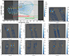 |
Fig. 1. Top-left panel: Projection of Ganymede’s FUV aurora acquired by Juno-UVS on June 7th, 2021, from 16:52 to 17:04 UTC. We used the Ganymede-centered Phi-Omega (GPhiO) frame of reference, with z parallel to Jupiter’s spin axis and y toward Jupiter; x completes the right-handed system. The brightness is integrated over 130.4 ± 1.5 nm and 135.6 ± 1.5 nm. The green lines show the predicted OCFB (Duling et al. 2022). The background shades of gray (from dark to light) represent the surface illumination: surface that is not illuminated, only sunlight reflected by Jupiter, only direct sunlight, and both reflected and direct sunlight. The green and red bars mark the direct and reflected illuminations, respectively. The red dot around 90° is the downstream direction, while the red cross at −90° is the upstream direction. The orange dot at 0° and the yellow star at ∼–40° are the direction to Jupiter and to the Sun, respectively. The numbers 1–9 mark successive Juno spins. The green cross is the projection of Juno’s closest approach. The orange boxes labeled a-g are reproduced in the seven panels, which show the patches observed along Ganymede’s aurora smoothed using a 3 × 3 Gaussian kernel with 2 sigma that approximately matches the ∼0.1° point spread function of UVS. We encircled the visually identified patches. The color levels are logarithmic; for panels a-g, we visually display 100R (S/N ∼ 1) as the lower level to highlight the beads. |
3. Results and discussion
The projections in panels a-g of Fig. 1 show that Ganymede’s aurora was fragmented into multiple patches of emission with a typical transversal size of approximately 50 km. These patches reach ∼200 R (1 Rayleigh = 1010 photons m−2 s−1), and they appear to be located only on the leading side of the moon. Juno did not observe the same morphology in the southern hemisphere, possibly because of Juno’s vantage point, as the southern aurora is observed at high emission angles (≳50°) and from farther away than the northern hemisphere. The vertical extension of Ganymede’s aurora was estimated to be 20–50 km (Greathouse et al. 2022a), and hence the high emission angle of the observations from the southern hemisphere could make the patches undistinguishable from Juno’s vantage point. Alternatively, the apparent asymmetry in the auroral morphology might be linked to Ganymede’s magnetic latitude and position with respect to the Jovian plasma disk (Saur et al. 2022). At the time of the Juno-UVS observations, Ganymede was at ∼302° System III longitude; assuming an axisymmetric plasma disk tilted by ∼7° toward 200° longitude (Phipps et al. 2020), Ganymede was inside the plasma disk ∼10 RG below its center. The orientation of Jupiter’s magnetic field encountered by Ganymede and the plasma environment along the open field lines connected to the moon might introduce asymmetries in the auroral emission between the two hemisphere, as they have been observed to produce asymmetries at Earth (Østgaard et al. 2005) and Europa (Roth et al. 2016).
The interaction between Ganymede’s magnetic field and Jupiter’s magnetospheres creates two regions: one at a low latitude marked by magnetic field lines closed at the moon and one at both poles, where open field lines connect Ganymede to Jupiter’s magnetosphere (Jia & Kivelson 2021). As Ganymede orbits more slowly than the magnetospheric flow, the flux tubes formed by the open field lines anchored at Ganymede are tilted in the direction of the plasma flow in Ganymede’s reference frame; therefore, the region of closed field lines is expanded on the upstream side and compressed on the downstream side (Duling et al. 2022). Ganymede’s aurora lies close to the open–closed field line boundary (OCFB) between the two regions, whose location mainly depends on the upstream plasma density, the pressure, and the atmospheric density. Duling et al. (2022) estimated the uncertainty on the OCFB position to be ∼7° on the downstream side, which is larger than the size of the patches, ∼1°. We adopted a magnetohydrodynamic model of Ganymede’s magnetosphere (Duling et al. 2014, 2022) to constrain the magnetospheric region connected to the patches. Figure 2 shows the magnetic field lines that intersect Ganymede at the same longitude as that of the patches; for each longitude, we produced two magnetic field lines bracketing the OCFB: one 1° poleward of the OCFB and the other 1° equatorward of the OCFB. The model shows that the patches originate somewhere between the outer part of the downstream magnetosphere and the downstream reconnection region (see, for example, Fig. 1 in Waite et al. 2024 for a sketch of those regions). The magnetic field lines are twisted compared to a dipolar field, as they bend under the interaction with Jupiter’s magnetosphere and the compression of Ganymede’s magnetosphere on the leading side.
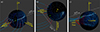 |
Fig. 2. Closed and open magnetic field lines (red and blue, respectively) near the OCFB of Ganymede’s magnetosphere. The feet of these lines are at the longitude of the auroral patches shown in Fig. 1 (one for each spin); the red lines start 1° equatorward of the OCFB, while the blue lines start 1° poleward. Juno-UVS observations performed during PJ 34 are projected onto Ganymede’s surface. The dashed white line is Juno’s trajectory, while the green cross is the projection of the spacecraft position during the closest approach. Panel a: 3D geometry of the magnetic field lines. Panels b and c: Projections as seen from above Ganymede and from Jupiter, respectively. |
The fragmentation of auroral arcs is commonly observed in auroras. At Earth, sub-storms are often preceded by the formation of auroral “beads” (Forsyth et al. 2020). Their precise generation and evolution is still debated, although they appear to originate in the magnetotail (Forsyth et al. 2020). Jupiter’s main emission is periodically affected by dawn storms, which can be accompanied by bead formation (Bonfond et al. 2021). Observations and models of the Earth’s system suggest that both the cross-field current instability (Lui et al. 1991) and the shear flow ballooning instability (Voronkov et al. 1997) are potential drivers of auroral beads (Kalmoni et al. 2015). Signatures of ripples associated with the ballooning-interchange instability in the night sector during sub-storms have been reported from simulations (Sorathia et al. 2020). Earth-based observations and models show that the size of the beads mapped to the magnetotail is comparable with the local ion gyroradius (Pritchett & Coroniti 1999; Yao et al. 2017). We used the magnetic flux conservation to estimate the size of the beads at Ganymede’s magnetotail (LT) from their approximate diameter at the surface, LS ≈ 50 km:  , where BS ≈ 800 nT and BT ≈ 80 nT are the surface and magnetotail field magnitudes, respectively. We obtained LT/2 ≈ 75 km, to be compared with the local gyroradius. Protons and H2+ require an energy of ∼1–3 keV to match the 75 km gyroradius, which is much larger than the few tens of eV observed around Ganymede (Bagenal & Delamere 2011; Valek et al. 2022). Instead, O+ and O2+ at 200 and 100 eV, corresponding to the typical heavy ion population in Ganymede’s magnetosphere, in a magnetic field of ∼80 nT have a gyroradius of ∼75 km, which matches the size of the beads. This suggests the ballooning instability is the driving mechanism. If so, we can expect a symmetric auroral morphology between the hemispheres, and therefore the lack of detection of patches in the southern aurora is probably caused by Juno’s viewing geometry. The size of the patches suggests that pick-up ions in the magnetospheric region are not involved in their formation, as their pick-up energy in a flow at 140 km/s would be > 1 keV. The observed size of the patches may be slightly overestimated, as the brightness S/N near their edges is ≲2. If we strictly consider S/N > 2 to determine the size of the patches, it decreases to ∼30–40 km, which does not change the conclusions of this work.
The auroral patches on Ganymede that are apparently similar to terrestrial beads suggests that fundamental physical process(es) could be generally driven by the coupling between a celestial body, its magnetosphere, and external forces. The dynamics of Ganymede’s magnetosphere is affected by its interaction with Jupiter’s magnetosphere, which is somewhat similar to the influence of the solar wind on Earth’s magnetosphere, and hence Ganymede represents a unique case for comparative studies.
4. Conclusions
We have reported Juno-UVS observations of Ganymede’s auroral patches observed on June 7th, 2021, that resemble terrestrial beads associated with sub-storms (Kalmoni et al. 2015) and Jovian beads that are observed before dawn storms (Bonfond et al. 2021). This suggests that the physical processes driving their formation could be a common feature of magnetospheric dynamics.
Juno-UVS observations have raised new questions about Ganymede’s aurora: How do the mesoscale auroral structures form and evolve over time? Does Ganymede exhibit events similar to sub-storms and dawn storms? What is Ganymede’s magnetospheric regime? Are there short-term variations in the OCFB location? What are the characteristics of the particle precipitation associated with the patches, and how are they accelerated? The Jupiter Icy Moons Explorer (Juice), en route to the Jovian system, is expected to arrive in 2031. It carries a UVS similar to Juno-UVS (Masters et al. 2025) and represents a precious opportunity to investigate the dynamics and variability of Ganymede’s aurora, as well as its magnetospheric processes.
Acknowledgments
This work is based on the master’s thesis of P. Gusbin revealing Ganymede’s auroral patches (Gusbin 2025). This work was supported by the Fonds de la Recherche Scientifique – FNRS under Grant(s) No. T003524F. B. Bonfond is a Research Associate of the Fonds de la Recherche Scientifique – FNRS. S. Duling has received funding from the European Research Council (ERC) under the European Union’s Horizon2020 research and innovation program (Grant agreement No. 884711). V. Hue and B. Benmahi acknowledge support from the French government under the France 2030 investment plan, as part of the Initiative d’Excellence d’Aix-Marseille Université – A*MIDEX AMX-22-CPJ-04, as well as the support of CNES to the Juno and JUICE missions. Greathouse was funded by the NASA’s New Frontiers Program for Juno via contract NNM06AA75C with the Southwest Research Institute. This work was funded by NASA’s New Frontiers Program for Juno via contract with the Southwest Research Institute.
References
- Bagenal, F., & Delamere, P. A. 2011, J. Geophys. Res.: Space Phys., 116 [Google Scholar]
- Benmahi, B., Hue, V., Vorbuger, A., et al. 2025, A&A, 703, A260 [NASA ADS] [CrossRef] [EDP Sciences] [Google Scholar]
- Bolton, S. J., Lunine, J., Stevenson, D., et al. 2017, Space Sci. Rev., 213, 5 [CrossRef] [Google Scholar]
- Bonfond, B., Yao, Z. H., Gladstone, G. R., et al. 2021, AGU Advances, 2, e2020AV000275 [Google Scholar]
- de Kleer, K., Milby, Z., Schmidt, C., Camarca, M., & Brown, M. E. 2023, Planet. Sci. J., 4, 37 [NASA ADS] [CrossRef] [Google Scholar]
- Duling, S., Saur, J., & Wicht, J. 2014, J. Geophys. Res.: Space Phys., 119, 4412 [Google Scholar]
- Duling, S., Saur, J., Clark, G., et al. 2022, Geophys. Res. Lett., 49, e2022GL101688 [Google Scholar]
- Feldman, P. D., McGrath, M. A., Strobel, D. F., et al. 2000, ApJ, 535, 1085 [NASA ADS] [CrossRef] [Google Scholar]
- Forsyth, C., Sergeev, V. A., Henderson, M. G., Nishimura, Y., & Gallardo-Lacourt, B. 2020, Space Sci. Rev., 216, 46 [Google Scholar]
- Gladstone, G. R., Persyn, S. C., Eterno, J. S., et al. 2017, Space Sci. Rev., 213, 447 [Google Scholar]
- Greathouse, T. K., Gladstone, G. R., Davis, M. W., et al. 2013, in SPIE Optical Engineering + {Applications}, eds. O. H. Siegmund, San Diego, California, United States, 88590T [Google Scholar]
- Greathouse, T. K., Gladstone, G. R., Molyneux, P. M., et al. 2022a, Geophys. Res. Lett., 49, e2022GL099794 [NASA ADS] [CrossRef] [Google Scholar]
- Greathouse, T. K., Gladstone, R., Versteeg, M. H., et al. 2022b, in AGU Fall Meeting 2022 (AGU) [Google Scholar]
- Gurnett, D. A., Kurth, W. S., Roux, A., Bolton, S. J., & Kennel, C. F. 1996, Nature, 384, 535 [Google Scholar]
- Gusbin, P. 2025, Ph.D. Thesis, Université de Liège, Belgique [Google Scholar]
- Hall, D. T., Feldman, P. D., McGrath, M. A., & Strobel, D. F. 1998, ApJ, 499, 475 [NASA ADS] [CrossRef] [Google Scholar]
- Hue, V., Randall Gladstone, G., Greathouse, T. K., et al. 2019, AJ, 157, 90 [NASA ADS] [CrossRef] [Google Scholar]
- Hue, V., Giles, R. S., Gladstone, G. R., et al. 2021, J. Astron. Telescopes Instrum. Syst., 7, 044003 [NASA ADS] [Google Scholar]
- Jia, X., & Kivelson, M. G. 2021, in Magnetospheres in the Solar System (American Geophysical Union (AGU)), 557 [Google Scholar]
- Kalmoni, N. M. E., Rae, I. J., Watt, C. E. J., et al. 2015, J. Geophys. Res.: Space Phys., 120, 8503 [Google Scholar]
- Kivelson, M. G., Khurana, K. K., & Volwerk, M. 2002, Icarus, 157, 507 [CrossRef] [Google Scholar]
- Lui, A. T. Y., Chang, C.-L., Mankofsky, A., Wong, H.-K., & Winske, D. 1991, J. Geophys. Res.: Space Phys., 96, 11389 [Google Scholar]
- Masters, A., Modolo, R., Roussos, E., et al. 2025, Space Sci. Rev., 221, 24 [Google Scholar]
- McGrath, M. A., Jia, X., Retherford, K., et al. 2013, J. Geophys. Res.: Space Phys., 118, 2043 [Google Scholar]
- Østgaard, N., Tsyganenko, N. A., Mende, S. B., et al. 2005, Geophys. Res. Lett., 32 [Google Scholar]
- Phipps, P. H., Withers, P., Vogt, M. F., et al. 2020, J. Geophys. Res. Space Phys., 125 [Google Scholar]
- Pritchett, P. L., & Coroniti, F. V. 1999, J. Geophys. Res.: Space Phys., 104, 12289 [Google Scholar]
- Roth, L., Saur, J., Retherford, K. D., et al. 2016, J. Geophys. Res.: Space Phys., 121, 2143 [Google Scholar]
- Saur, J., Duling, S., Roth, L., et al. 2015, J. Geophys. Res.: Space Phys., 120, 1715 [NASA ADS] [CrossRef] [Google Scholar]
- Saur, J., Duling, S., Wennmacher, A., et al. 2022, Geophys. Res. Lett., 49, e2022GL098600 [Google Scholar]
- Sorathia, K. A., Merkin, V. G., Panov, E. V., et al. 2020, Geophys. Res. Lett., 47, e2020GL088227 [Google Scholar]
- Trantham, B. 2014, Juno Jupiter UVS Raw Data Archive V1.0 [Google Scholar]
- Valek, P. W., Waite, J. H., Allegrini, F., et al. 2022, Geophys. Res. Lett., 49, e2022GL100281 [Google Scholar]
- Vorburger, A., Fatemi, S., Carberry Mogan, S. R., et al. 2024, Icarus, 409, 115847 [NASA ADS] [CrossRef] [Google Scholar]
- Voronkov, I., Rankin, R., Frycz, P., Tikhonchuk, V. T., & Samson, J. C. 1997, J. Geophys. Res.: Space Phys., 102, 9639 [Google Scholar]
- Waite, J. H., Greathouse, T. K., Carberry Mogan, S. R., et al. 2024, J. Geophys. Res.: Planets, 129, e2023JE007859 [NASA ADS] [CrossRef] [Google Scholar]
- Yao, Z., Pu, Z. Y., Rae, I. J., Radioti, A., & Kubyshkina, M. V. 2017, Geosci. Lett., 4, 8 [Google Scholar]
All Figures
|
Fig. 1. Top-left panel: Projection of Ganymede’s FUV aurora acquired by Juno-UVS on June 7th, 2021, from 16:52 to 17:04 UTC. We used the Ganymede-centered Phi-Omega (GPhiO) frame of reference, with z parallel to Jupiter’s spin axis and y toward Jupiter; x completes the right-handed system. The brightness is integrated over 130.4 ± 1.5 nm and 135.6 ± 1.5 nm. The green lines show the predicted OCFB (Duling et al. 2022). The background shades of gray (from dark to light) represent the surface illumination: surface that is not illuminated, only sunlight reflected by Jupiter, only direct sunlight, and both reflected and direct sunlight. The green and red bars mark the direct and reflected illuminations, respectively. The red dot around 90° is the downstream direction, while the red cross at −90° is the upstream direction. The orange dot at 0° and the yellow star at ∼–40° are the direction to Jupiter and to the Sun, respectively. The numbers 1–9 mark successive Juno spins. The green cross is the projection of Juno’s closest approach. The orange boxes labeled a-g are reproduced in the seven panels, which show the patches observed along Ganymede’s aurora smoothed using a 3 × 3 Gaussian kernel with 2 sigma that approximately matches the ∼0.1° point spread function of UVS. We encircled the visually identified patches. The color levels are logarithmic; for panels a-g, we visually display 100R (S/N ∼ 1) as the lower level to highlight the beads. |
| In the text | |
|
Fig. 2. Closed and open magnetic field lines (red and blue, respectively) near the OCFB of Ganymede’s magnetosphere. The feet of these lines are at the longitude of the auroral patches shown in Fig. 1 (one for each spin); the red lines start 1° equatorward of the OCFB, while the blue lines start 1° poleward. Juno-UVS observations performed during PJ 34 are projected onto Ganymede’s surface. The dashed white line is Juno’s trajectory, while the green cross is the projection of the spacecraft position during the closest approach. Panel a: 3D geometry of the magnetic field lines. Panels b and c: Projections as seen from above Ganymede and from Jupiter, respectively. |
| In the text | |
Current usage metrics show cumulative count of Article Views (full-text article views including HTML views, PDF and ePub downloads, according to the available data) and Abstracts Views on Vision4Press platform.
Data correspond to usage on the plateform after 2015. The current usage metrics is available 48-96 hours after online publication and is updated daily on week days.
Initial download of the metrics may take a while.