| Issue |
A&A
Volume 707, March 2026
|
|
|---|---|---|
| Article Number | A36 | |
| Number of page(s) | 11 | |
| Section | Planets, planetary systems, and small bodies | |
| DOI | https://doi.org/10.1051/0004-6361/202451954 | |
| Published online | 27 February 2026 | |
Small-scale magnetic field effects on individual spectral line radial velocities in the photosphere and chromosphere of the Sun
1
Department of Physics and Astronomy, Uppsala University,
Box 516,
75120
Uppsala,
Sweden
2
Institute for Solar Physics, Dept. of Astronomy, Stockholm University, AlbaNova University Centre,
106 91
Stockholm,
Sweden
★ Corresponding author: This email address is being protected from spambots. You need JavaScript enabled to view it.
Received:
22
August
2025
Accepted:
9
November
2025
Abstract
Context. Advancements in extreme-precision radial velocity (RV) observations for detecting low-mass exoplanets show that different spectral lines show different behaviours in response to stellar activity. Though this can be dealt with experimentally, why this is the case has not been studied. The Sun is a good test case for testing hypotheses as we can study spatially resolved observations with high-resolution spectropolarimetry to understand spectral line behaviour.
Aims. We aim to investigate whether the difference of spectral line behaviour can be attributed to the height of atoms in the solar atmosphere. It is expected that photospheric spectral lines will act differently from their chromospheric counterparts in response to magnetic fields.
Methods. We used a unique dataset using the CRisp Imaging SpectroPolarimeter (CRISP) looking at three spectral lines, two in the photosphere and one in the chromosphere, and measured their spatially resolved radial velocities, their transversal and longitudinal magnetic fields, their magnetic field strengths, and their source functions. We correlated the magnetic field measurements against the radial velocities and compared them against the case in which we destroyed the spatial resolution to mimic a normal stellar observation with high-resolution spectra.
Results. We find that the unsigned magnetic field is strongly correlated to the RV for both the photospheric and chromospheric spectral lines in the case where the observation is spatially resolved. When the spatial resolution is destroyed, this correlation changes. We find that for the photospheric spectral lines there still exists a correlation to both components of the magnetic field, but the chromospheric spectral lines do not show any significant correlation.
Key words: Sun: chromosphere / Sun: photosphere / planets and satellites: detection
© The Authors 2026
 Open Access article, published by EDP Sciences, under the terms of the Creative Commons Attribution License (https://creativecommons.org/licenses/by/4.0), which permits unrestricted use, distribution, and reproduction in any medium, provided the original work is properly cited.
This article is published in open access under the Subscribe to Open model. This email address is being protected from spambots. You need JavaScript enabled to view it. to support open access publication.
1 Introduction
A significant hurdle in the field of exoplanet science is in the measurement of extreme precision radial velocities (EPRVs) of stars for the purpose of find true-Earth analogues (Crass et al. 2021). These Earth twins have signals of 10 cm/s or lower, depending on the orientation of the system. In this regime, however, there exist many different sources of RV noise that can each mimic or obscure planetary signals. These sources exist in three categories: photon noise, instrument instabilities, and stellar variability. Photon noise represents the minimum possible uncertainty in an observation, defined by various aspects of a measurement such as target brightness, telescope size, spectral resolution of the instrument, observing conditions, and the number of useful spectral lines (Bouchy et al. 2001). The instrumental effects include all uncertainties coming from the instrument hardware and software, such as stability of the spectral format, variation in the point spread function (PSF) across the detector, detector noise and linearity properties, and the data reduction pipeline. The instrumental effects used to be the dominant sources of RV uncertainty in previous surveys, but modern facilities such as the Echelle SPectrograph for Rocky Exoplanet and Stable Spectroscopic Observations (ESPRESSO, Pepe et al. 2021), the EXtreme PREcision Spectrograph (EXPRES, Fischer et al. 2017), NN-EXPLORE Exoplanet Investigations with Doppler Spectroscopy (NEID; Schwab et al. 2016), and the upcoming High Accuracy Radial velocity Planet Searcher 3 (HARPS3, Thompson et al. 2016) will bring the instrumental RV precision to or even below 10–20 cm s−1 (Hall et al. 2018). New calibration systems involving laser frequency combs (LFCs) and simultaneous calibrations significantly improves instrument stability and new or improved methods of stabilizing the spectrograph has led to stellar variability becoming the dominant source of uncertainty (Crass et al. 2021).
We have a limited knowledge of physical processes in Sunlike stars in the context of how their intrinsic variability, driven by convection, differential rotation, magnetic fields, and surface inhomogeneities induce RV variations with amplitudes as high as 100 m/s and timescales ranging from seconds to decades (Klein et al. 2024). Some of these signals are correlated with the stellar rotation that can mimic close-in planets. Stellar surface velocity fields manifest themselves as transformations of the spectral line shape that can be interpreted as RV shifts using the traditional method of cross-correlating observations with a template and determining the RV from the centre of the resulting cross-correlation function (CCF). It was shown that one of the most dominant sources of RV uncertainty comes from the suppression of convection blueshift in magnetic regions of lower activity, Sun-like stars (Meunier et al. 2010b; Dumusque et al. 2014; Haywood et al. 2016; Bauer et al. 2018), which can lead to over 1 m sec−1 offsets in RV measurements.
Stellar variability is generally less important for detecting larger planets on shorter orbits, such as hot Jupiters, where the RV signal is in the tens to hundreds of metres per second, but it quickly becomes the dominant problem when hunting for Earth-like planets in Earth-like orbits around Sun-like stars, with typical RV amplitude of approximately 10 cm/s. To put this in perspective, for the HARPS3 instrument, this signal shows itself as a shift of all lines on the detector plane by a bit less than one nanometre when the pixel size is fifteen microns wide. Any unknown effect that causes the determination of the line centres to shift by less than one thousandth the size of a detector pixel will destroy any possibility of detecting Earth-like planets.
One of the difficulties in understanding the physical processes of Sun-like stars is that we only see the combined effect on the disc-integrated spectrum, while the surface velocity field is highly inhomogeneous. Though techniques are being developed to better understand the statistical properties of this kind of data, it is still nearly impossible to predict the precise impact on the derived stellar RV. New advancements in the field of EPRV have shown that individual spectral line RVs show different jitter responses to the stellar surface velocity fields, while all lines react similarly to the orbital motion of the star. The differential analysis between the line groups can be used to separate the jitter even without a complete physical understanding of the cause (Dumusque 2018); for example, one can separate lines with large RV jitter from lines with small RV jitter, which can be used to minimize the impact of stellar activity. This can be combined with advanced data post-processing of time series, such as YARARA (Cretignier et al. 2021), which can partially separate jitter and orbital RV variation using principal component analysis (PCA). Additional work attempts to understand how to mitigate the effects of different noise sources, from extracting measures of the suppression of convective blueshift (Miklos et al. 2020), to using spot models to de-trend RV variations from stellar activity (e.g. Siegel et al. 2024; Dorval & Snellen 2024), to using neural networks to remove stellar activity signals from RV measurements (de Beurs et al. 2022). However, it is likely that future RV surveys will use a combination of methods in order to best reduce noise in observations (e.g. with the EXPRES stellar signals project, Zhao et al. 2022)
Alternatively, we can study the one star where we can obtain spatially resolved data – the Sun – with one of the many modern instruments performing disc-integrated observations such as, for example, HARPS-N, HARPS, EXPRES, and NEID. By taking spatially resolved data, we can look at physical processes that we know have an effect and test how they affect the RVs of the observation at different timescales to probe different stellar activity effects. Previous studies have already observed the Sun as a disc-integrated source (e.g. Meunier et al. 2010a; Haywood et al. 2016; Milbourne et al. 2019) and compared simultaneous disc-integrated spectral measurements and images of the solar surface and estimating solar activity which confirmed that the inhibition of convection due to active regions is the dominant source of activity-induced RV variations. Such studies have also found that activity-driven RV variations are correlated with the full-disc magnetic flux density of the Sun, suggesting that this could be an effective method of mitigating RV noise.
In this study we aim to further address if the RV variability, referred to as jitter, of spectral lines can be uniquely attributed to their formation depths and magnetic structures in the stellar atmospheres. The Sun offers a unique opportunity to study this question with spatially resolved spectropolarimetry. By combining high spatial and spectral resolution, we can examine how local magnetic field structures correlate with RVs across different line-formation layers. For this purpose, we use a dataset obtained with the CRisp Imaging SpectroPolarimeter (CRISP, Scharmer et al. 2008) at the Swedish Solar Telescope (SST, Scharmer et al. 2003). We analyse three spectral lines: the Fe I 630.15 nm and Fe I 630.25 nm lines formed in the photosphere, and the Ca II 854.209 nm line which probes the chromosphere. These observations are taken in snapshots with a field of view (FoV) of 60″by 60″across the equatorial plane of the Sun. We explore their reaction to the local manifestation of magnetic activity as well as the global effect on radial velocity jitter. Using these lines we attempt to connect magnetic field orientation with the velocity field of matter at different stellar layers in order to provide further insights into the physical origin of stellar RV jitter with direct relevance for interpreting EPRV signals. The observational dataset used in this study is explored in Section 2, with the methods explained in Section 3. The results of this study are shown in Section 4 and are discussed in detail in Section 5.
2 Observations
The dataset used in this study was obtained with the CRISP (Scharmer 2006; Scharmer et al. 2008) instrument mounted on the Swedish 1-m Solar Telescope (Scharmer et al. 2003) on 2 July 2022 between 09:02 and 10:16 UT. We acquired a mosaic of 47 spatially resolved pointings along the solar equator covering a total FoV of approximately 1920″ by 60″. Each individual pointing spans ~60″× 60″, sampled at 0.07″ per pixel. Each observation is taken at a different μ angles, with μ = cos θ, and θ as the heliocentric angle, spanning near-disc-centre to limb angles, allowing for sampling of quiet and active regions at different line of sight geometries. The combined Stokes I mosaic of all 47 observations is shown in Fig. 2, with the observations being split into four lines for readability. To the upper right of each observation square in the mosaic we give the limb distance parameter, μ, which is the cosine of the angle between local radius at the centre of the image and direction to the observer. For each observation all Stokes parameters are extracted with Stokes Q and U probing linear polarization and Stokes V probing circular polarization.
CRISP is a dual-etalon Fabry–Pérot instrument operating in a telecentric configuration, allowing us to acquire data over a FoV of approximately 60″ × 60″ within a very narrow spectral passband. Due to small surface imperfections in the etalons, small wavelength shifts (cavity errors) are introduced across the FoV, which are corrected using flat-field calibration frames and removed prior to the estimation of the line of sight velocity. For a full description of CRISP, we refer the reader to Scharmer et al. (2026).
The dataset consists of spectral scans performed in the Fe I 6301 and 6302 Å and in the Ca II 8542 Å lines for each pointing of the mosaic. The data were processed using the SSTRED pipeline (de la Cruz Rodríguez et al. 2015; Löfdahl et al. 2021). Atmospheric distortions in the data were compensated for using the multi-object-multi-frame-blind-deconvolution method (Löfdahl 2002; Van Noort et al. 2005). The polarimetric calibration was performed using the field-dependent methods developed by van Noort & Rouppe van der Voort (2008). Fig. 1 shows the response function, the derivative of the intensity relative to a physical parameter at each depth point, for both sets of lines. To generate this example, the line-of-sight component of the magnetic field was set to 400 G constant at all depth points.
While CRISP is primarily designed for spectropolarimetry, its RV precision is limited compared to a dedicated RV instrument. With relatively few spectral lines and due to the Fabry–Pérot-based scanning, the RV uncertainties are typically of the order of tens of meters per second. However, the angular resolution of CRISP allows one to distinguish coherent parcels of gas moving at velocities well in excess of several hundred meters per second, and so the relative RV precision of CRISP is extremely high, reaching 1% or better. This level is more than sufficient to detect correlations between velocity fields and magnetic structures targeted in this study.
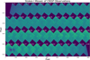 |
Fig. 1 Intensity map in Stokes I of all 47 observations. The mosaic is split into four parts for readability. Observations are taken from the western to eastern sides of the Sun. No merging images into a single mosaic using the overlap regions was attempted. To the upper right of each observation square is the μ value of each observation. All observations shown here come from the Stokes I observations of the Fe I 6301 Å line with a matched colour bar, with brighter colour showing more flux. |
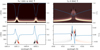 |
Fig. 2 Response function of the Fe lines (left) and the Ca line (right). The top shows the derivatives of the Stokes I relative to the gas temperature and the bottom shows the derivatives of the Stokes V relative to Bz. The synthetic profile is over-plotted in blue. |
3 Methods
Before the analysis the wavelength scales of 2D line profile maps were adjusted according to the cavity calibration map to remove the instrumental effects and allow comparison with a single frame and between the frames. The cavity error map in this context is the variation in the Fabry-Pérot cavity spacing D across the FoV, which leads to a shift of the wavelength by δλ = δDλ/D. For a full discussion of errors introduced via CRISP and the data reduction, refer to de la Cruz Rodríguez et al. (2015).
To investigate correlations between local magnetic fields and line-of-sight velocities in the solar atmosphere, we used high-resolution spectropolarimetric observations of three spectral lines: Fe I 630.15 nm, Fe I 630.25 nm (photosphere), and Ca II 854.209 nm (chromosphere). For each pixel in the spatially resolved FoV, we computed two components:
Radial velocity (RV): For the Fe lines, RVs were obtained from a Milne–Eddington inversion, appropriate for photospheric lines formed over narrow height ranges and monotonic temperature gradients, in which the line-of-sight velocity is a free parameter. This inversion provides a more stable RV estimate than centroiding in the presence of complex line asymmetries. A centre-of-mass calculation of the RVs applied to the Stokes I profile was also performed on the Fe lines to test if such a calculation would be valid for the Ca line that was formed in the chromosphere, and as such the Milne–Eddington inversion was not valid. The comparison showed that though there were minor differences, it would be appropriate to use the centre-of-mass derived RVs. Though the Ca line is biased due to a large number of data points on one side, each observation is similarly biased, and more accurate RV data measurements can be obtained by subtracting through averaging and normalization. Although this method is more sensitive to pixel-level noise, normalization and bias correction allow for robust comparisons across the dataset. The Ca II line was also separated into three components: the core of the Ca line and the wings of the Ca line to test different heights in the solar atmosphere, and the entire Ca line.
Magnetic field components: Longitudinal (Bz) and transversal (Bt) magnetic fields were derived from the Stokes V and (Q, U) profiles, respectively, assuming weak-field approximations where applicable (Auer et al. 1977). From these, we also estimated the total magnetic field strength, |B|.
To enable a fair comparison between different observations and line types, all RV and magnetic field maps are scaled to a common range by subtracting the median and normalizing the maximum value to one. We then performed a spatial correlation analysis to quantify the relationship between the RV maps and different magnetic field maps. We computed two separate correlations:
2D cross-correlations: These were computed between spatially resolved maps of RVs and magnetic field components for each observation. Both signed and unsigned quantities were considered, whereby the signed correlations preserve the directionality of flows and the field polarity, whereas the unsigned correlations reflect the magnitude of the field regardless of sign. The correlation maps were computed by shifting one map over the other by up to ±50 pixels in both x and y directions and computing the normalized cross-correlation at each shift. A strong central peak (i.e. at zero shift) indicates a tight spatial correspondence between the RV and magnetic field structures.
1D correlations: These were computed after spatially averaging the full Stokes I, Q, U, and V cubes into a single spectrum for each observation – a process that mimics spatially unresolved stellar observations. For each averaged frame, we extracted a single RV and magnetic field value and then computed the correlation across all 47 pointings. Similar to the 2D maps, a strong central peak indicates a strong correspondence between magnetic field measurements and RVs.
There is an important trade-off between RV precision, spectral resolution, and spatial resolution in this study. As is stated in Section 2, CRISP is not optimized for extreme RV precision; errors in RV retrieval from CRISP data are typically at the level of tens of meters per second, due to cavity errors in the Fabry–Pérot etalons, pixel-to-pixel variability, and photon noise in individual Stokes profiles. Another important aspect is that the wavelength errors in CRISP have stable and smooth patterns across a stack of images taken in the same position, assuming that the spatial resolution stays the same. This allows for the meaningful comparison of correlations across different images. CRISP offers a high spatial resolution (with a FoV of 60″ by 60 ″ and a pixel size of 0.07 ″) and spectral resolution (R ≈ 105 000 at 6302 Å). For reference, studies have shown that the average size of a solar granule can be between 0.17″ to 2.15″ (Roudier & Muller 1986). Combined with excellent spectropolarimetric capabilities and an estimated noise level for the Stokes profiles of around 2 × 10⁻³ for Stokes Q/Ic, U/Ic, and V/Ic (Ortiz & Rouppe van der Voort 2010), CRISP is an ideal instrument with which to study correlations between magnetic and velocity fields and how these gradually decay with the decrease of spatial resolution.
The analysis was primarily focused on correlation between velocity and magnetic fields, but it is important to note that the relation between Stokes parameters Q, U, and V and magnetic field strength and orientation also depends on change of the source function along the line formation depth. In order to determine if the CCF with the velocity field is dominated by the magnetic field or by the source function gradient, we calculated a Milne–Eddington inversion (de la Cruz Rodríguez 2019) on the 2D data. This is essentially a least squares fit of the spectra using a Milne–Eddington model atmosphere with model parameters being the three components of the magnetic field, the total Doppler width, line-of-sight velocity, line-to-continuum opacity ratio, damping parameter, and the two parameters describing a linear source function, Sν = S0 + S1τ, where S0 is the source function at τ = 0 and S1 is the gradient of the source function with optical-depth. pyMilne utilizes a Levenberg-Marquardt algorithm to perform the fitting. Milne–Eddington inversions are commonly used in solar physics (see, e.g. del Toro Iniesta 2003) and it is part of the data processing pipeline for space missions such as Solar Orbiter (the PHI instrument) (Solanki et al. 2020), the Solar Dynamics Observatory (the HMI instrument) (Scherrer et al. 2012), or Hinode (the SOT instrument) (Tsuneta et al. 2008).
The Milne–Eddington model assumes an atmosphere with a linearly varying source function (with optical depth) and all the other parameters are assumed to be constant with depth. By assuming this model, it is possible to derive an analytical expression of the polarized radiative transfer equation. These assumptions work relatively well with photospheric lines that are sensitive to a thin range of heights in the atmosphere (300 km). The temperature stratification is usually monotonically decreasing with height in the photosphere, and therefore a linear source function can suffice to model the source function of photospheric lines. Although in reality all other model parameters may change as a function of depth, they can be approximated by a constant value because they are expected to change slowly within the formation range of the line.
The resulting model includes the strength and orientation of magnetic field, the line-of-sight velocity, the optical depth of the line, the damping coefficient, and the linear approximation for the source function dependence on the optical depth, τ (S = S0 + S1τ) (Auer et al. 1977; Landolfi & Landi Degl’Innocenti 1982), with S0 being the initial value of the source function and S1 being the gradient of the source function. The inversion is done for every pixel in the original image. We have assessed possible interplays between the source function and the magnetic field, by calculating 2D correlation of the line-of-sight velocity with magnetic field strength. The Milne–Eddington approximation works well for the photospheric lines of iron, whereas the assumption of a linear source function cannot capture the complexity of the stratification of the real source function including a photosphere and a chromosphere. Ca II 8542 is a very strong line that samples the photosphere in wings and the chromosphere close to line centre, which usually translates into sampling a range of heights of at least 1500 km). The approximations adopted by the Milne–Eddington model cannot capture the complex changes of the real physical parameters with depth that such range would require: model parameters cannot be realistically assumed to be constant with height. The linear approximation of the source function poses a too simplistic shape for such a large height range, where both LTE and non-LTE conditions must be captured in the source function stratification.
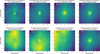 |
Fig. 3 Averaged correlations between the RVs and either the longitudinal or transversal magnetic fields derived from the Fe I 6302.15 and Ca II 8542 Å lines. The active averages were taken from observations 23, 35, and 36. The quiescent averages were taken from all remaining observations except for observations 0 and 46. |
4 Results
The complete unsigned 2D correlation figures are shown in Figs. A.1–A.4, with the observation number and signal-to-noise ratio (S/N), calculated via comparing the amplitude of the peak to the variability of the 2D map without the peak above each figure. Observations 23, 35, and 36 correspond to regions containing large sunspots. All correlation maps have been scaled so that the minimum is at zero and the maximum is at one. A representative summary is shown in Fig. 3, which plots the average of the correlation functions between RVs and either the longitudinal (Bz) or transversal (Bt) magnetic fields derived from the Fe I 6302.15 and Ca II 8542 Å lines.
In quiescent regions, the Ca II line shows a clear peak in the 2D correlation with Bt at zero spatial offset, indicating a strong spatial correlation between regions of enhanced tangential magnetic field and high absolute RV values. This suggests that even in the chromosphere, magnetic field structures influence local velocity fields. The detection significance, C, was calculated as the ratio of the peak correlation amplitude at zero shift to the standard deviation of the entire 2D map.
In active regions, while some residual correlation is visible, the signal is weaker and less statistically significant – likely due to the disruption of convective flows and greater structural complexity in sunspots and faculae. Correlations involving Bz are generally weaker or absent in both lines.
Figure 4 further illustrates the spatial structure of the correlation, showing observation 25 (a quiescent region near disc centre). Radial velocities align with bright granules, while Bz maps trace intergranular lanes, consistent with magnetic flux concentration in downflow regions, while the Bt field appears more diffuse.
This spatial co-location between convective flows and magnetic features supports the interpretation that RVs are locally modulated by small-scale fields. These signatures would be averaged out in unresolved stellar spectra but can still induce net shifts depending on line formation depth.
To approach disc-integrated (Sun-as-a-star) observations, we computed 1D correlations across binned observations. Figure 5 shows the normalized RV, Bz, and Bt values for each pointing, while Fig. 6 shows their respective correlations. The Fe lines show significant correlations (detection significance C > 3) between RV and both Bz and Bt, indicating that even in spatially unresolved data, small-scale magnetic structures contribute to net RV shifts–particularly in the photosphere. In contrast, the Ca II line shows no statistically significant correlation, implying that chromospheric features average out in integrated light.
To probe the effect of line formation height, we split the Ca II 8542 Å line into core (chromospheric), wing (photospheric), and full-profile components to sample a range of heights of at least 1500 km. As is shown in Fig. 7, the correlation with Bz is weak and noisy for the individual components, with C < 3. When the full line profile is used, the noise averages out and a clearer signal emerges. When the full profile is used to derive the magnetic field, the recovered 2D maps look more photospheric and the structures look more confined than when using the core. Here, the magnetic field has expanded due to the lower gas pressure and is observed as weaker. This could be due to one of two factors: a lower S/N of the isolated profiles, which should be tested in later studies, or the fact that magnetic features are more concentrated and that gives a higher correlation. Later analysis takes the entire Ca line as the input when calculating RV, Bz, and Bt.
Figure 8 compares the correlation of RVs with magnetic field strength (|B|) and source function parameters (S0, S1) derived from the Milne–Eddington inversion. The peak in the |B| correlation and the weak anti-correlation with S0 and S1 suggest that the observed RV variations are primarily driven by magnetic fields rather than radiative transfer artefacts. This supports the physical validity of the observed correlations and reinforces that the measured RV–magnetic field relationships reflect genuine atmospheric dynamics.
From this, we can make the following conclusions:
As was expected from solar granulation dynamics, small-scale magnetic fields are concentrated in intergranular lanes;
One cannot simply take the Stokes Q, U, V signals as direct proxies of the magnetic field strength as the Stokes parameters are also modulated by the gradient of the source function. In the case of this study, the difference between a more in-depth analysis of the magnetic field and one using proxies derived from the Stokes parameters is small;
In spatially resolved data, quiescent regions show strong correlations between the unsigned RVs and the unsigned Bz and Bt fields. This effect is suppressed when considering more active regions with spots where there is no significant correlation, with further study on a dataset with more faculae present providing detail on if this is true for faculae as well;
In spatially unresolved data, active regions remain correlated to RV effects in photospheric lines. This effect is greatly diminished for chromospheric lines, even when considering lines that extend into the photosphere.
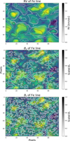 |
Fig. 4 Fragment of intensity image from observation 25 corresponding to the quiescent region of the photosphere close to the disc centre. Over-plotted are the contours of the absolute values of RV (top), longitudinal magnetic field (middle), and transversal magnetic field (bottom). Darker contours correspond to higher values. |
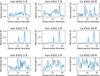 |
Fig. 5 Computed values of RV, Bz, and Bt when observations are binned into one data point. Similar to the 2D case, absolute values are taken of the radial velocities and Bz. Observations 23, 35, and 36 contain magnetically active regions. |
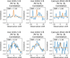 |
Fig. 6 Correlations of radial velocities derived from the three individual lines against magnetic field components Bz and Bt, when each observation has been binned to a single data point in Stokes IQUV. Observations are correlated against each other, and correlation values normalized. |
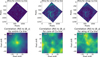 |
Fig. 7 Comparisons of the correlations of the longitudinal magnetic field to the RVs derived from the Ca II 8542 Å line. The RVs were calculated using either the entire line profile (left column), the core of the line (|Δλ| < 0.3 Å, middle column), or just the wings (|Δλ| > 0.3 Å, right column). All figures are based on the 28th pointing. |
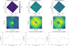 |
Fig. 8 Magnetic field strength |B|, and the source function fit coefficients S0 and S1 (top row) and their correlations to the absolute value of RVs (middle row). 1D slices taken through the middle of the 2D correlation plots portray the relative correlation strengths (bottom row). All figures are based on the 33rd pointing. |
5 Discussion
In quiescent regions of the Sun, small-scale magnetic fields cause significant RV fluctuations that can be easily seen using the unsigned spatially resolved data in Figs. A.1–A.4, excluding observations 23, 35, and 36. The transversal magnetic field and the unsigned longitudinal magnetic field are generally correlated to the absolute values of the RV measurements. This is true for structures found in the photosphere and those found in the chromosphere. This is consistent with the expected behaviour of solar granulation: horizontal fields in upflowing granules, and vertical fields in intergranular downflows, as is illustrated in Fig. 4.
In active regions, this correlation weakens or disappears. Strong magnetic fields alter or suppress convective patterns; for example, the blocking of convection in sunspot umbrae or distortion in penumbrae via the Evershed flow (Scharmer 2009; Esteban Pozuelo et al. 2015). Thus, magnetic fields in active regions disrupt the fine-scale structures that normally generate RV-field correlations in quiescent areas. Although correlation peaks remain visible in the 2D CCFs, they are less pronounced and often accompanied by secondary peaks. These are likely artefacts of reduced signal strength and increased noise in the RV maps within active regions, amplified by the CCF normalization.
In order to confirm that these effects are due solely to the magnetic field, and not to the correlation with the vertical gradient of the source function, we expanded this study and calculated the magnetic fields and sources functions using a Milne–Eddington inversion. This returned the 2D RV map, the magnetic field strength, and the source functions S0 and S1 solely for the Fe lines in the photosphere. We could not do the same calculation on the chromospheric Ca II due to the breakdown of the limiting assumptions of the Milne–Eddington atmospheric model, relating to the linear dependence of the source function on the optical depth, further discussed in Section 3. The result (Fig. 8) is that the magnetic field strength shows a strong correlation with the RV, while the source function fitting parameters show only a weak anti-correlation with RV measurements. This confirms our conclusion about there being a significant correlation between RV and magnetic field strength.
There is a difference between the photospheric and chromospheric data, with there being a strong correlation between the transversal magnetic field and the absolute RV for the Ca II line even in active regions. This may reflect the physical conditions of the chromosphere relating to the nature of the pressure balance. The plasma β = Pg/PB = 1 layer, defined by the ratio of gas pressure, Pg, and magnetic pressure, PB, is located within the lower chromosphere and it usually decreases moving upwards. Therefore, most of the features observed in the core of the λ8542 line sample a low-beta plasma region where magnetic forces are usually dominant over gas pressure gradients. The latter manifests in the intensity images as very filamentary structures that are aligned with the magnetic field vector (de la Cruz Rodríguez & Socas-Navarro 2011; Leenaarts et al. 2015; Asensio Ramos et al. 2017). Additionally, the frozen-in flux plasma condition usually holds in the chromosphere (see e.g. Priest 2014), explaining the strong correlation between the magnetic field and the observed velocities in network patches and active regions (e.g. Kianfar et al. 2020).
The problem as we understand it is the complexity of the phenomenon: the local velocity field is set by the 3D convective motions, affected by magnetic fields and its time evolution. For stars other than the Sun, all these effects are mushed together by the lack of angular resolution, with complicated weights due to geometry (the position on the visible disc) and stellar rotation. This complexity prompted projects two opposite approaches to the problem: using ab initio modelling or looking for statistical correlations with a rather weak connection to the physical mechanisms. Magnetohydrodynamic (MHD) models are not yet realistic enough to predict the changes in global RV values but there is a clear progress in this direction, illustrated by the consistency between observations and synthetic observables derived from MHD models with a minimal number of free parameters (e.g. Kunovac et al. 2025). The statistical side is technically simpler and we see many groups and tools that focus on describing perturbations of the velocity fields with toy models of active regions (e.g. Zhao & Dumusque 2023), Gaussian processes, and machine learning (e.g. Barragán et al. 2022; de Beurs et al. 2024; Rescigno & Al Moulla 2025), and using PCA of the time series (e.g. Cretignier et al. 2020).
One of the most significant findings of this study is that even after spatial averaging – mimicking stellar observations – photospheric lines retain a measurable correlation between RV and magnetic field strength, while the chromospheric lines do not (Fig. 6). This supports the idea that small-scale magnetic activity in the photosphere contributes to RV variability even for disc-integrated stellar flux observations, while chromospheric contributions largely cancel out. The small-scale magnetic fields still affect the RV measurements to a significant degree on the surface of a star, but, as was assumed, they are insignificant in the chromosphere in the case of observations of disc-integrated spectra. This is a marked departure from what we see in the spatially resolved data, where there is a strong correlation in quiescent regions of the Sun between the magnetic field and RVs.
This can help explain previously seen effects in EPRV studies. Dumusque (2018) and later follow-up studies by Cretignier et al. (2020) and Al Moulla et al. (2022) showed that there exist three separate groupings of individual lines. Some lines show a strong dependence on the activity of the star, some a mild dependence, and some no dependence. This effect was not studied in detail, but offered more as an empirical observation. Based on this work, a hypothesis can be made that the small-scale magnetic field in the photosphere causes a net global effect in RV that is not true for spectral lines present in the chromosphere.
The findings open four promising directions for further investigation:
- 1
Multi-line, multi-height CRISP analysis: Using additional spectral lines at different formation heights (either from archival CRISP datasets or coordinated observations), one could track how RV–field correlations evolve with altitude in the solar atmosphere. This would strengthen the link between formation height and activity sensitivity;
- 1
Modeling stellar line groupings: The empirical line classifications in Dumusque (2018) could be re-analysed using stellar atmosphere models that include detailed height stratification and magnetic field structures. Comparing modelled and observed RV–activity relations across different stellar types would generalize our results beyond the Sun;
- 1
A third avenue is to further investigate the effect of spatial resolution degradation directly – by artificially binning CRISP data to lower resolutions and assessing how correlation strength evolves. This would help us estimate the scale at which RV jitter from magnetic fields becomes negligible or unresolved;
- 1
A fourth question raised during this analysis is why there is not a clear signature that the tangential field blocks line-of-sight motions. For magnetic network patches and plage regions, the magnetic field is strongly vertical. These regions will likely have the strongest impact on correlations (Buehler et al. 2015; Morosin et al. 2020; Martínez González et al. 2012). In the case of a weak tangential field, there should be almost no correlation. Further observations focused primarily on these regions will be able to better answer this question.
In any case, we put forward a new hypothesis that small-scale magnetic fields have a significant effect on spectral lines present in the photospheres of stars, and no significant effect on spectral lines present in the chromospheres of stars. This study shows further reasons why spectropolarimetry is important in understanding RV jitter arising from stellar noise signals and offers ideas on how to further study this effect.
Acknowledgements
We have benefited greatly from the publicly available programming language Python, including the numpy Oliphant (2006–), matplotlib Hunter (2007), scipy Jones et al. (2001–). The Swedish 1-m Solar Telescope is operated on the island of La Palma by the Institute for Solar Physics of Stockholm University in the Spanish Observatorio del Roque de los Muchachos of the Instituto de Astrofísica de Canarias. The Institute for Solar Physics is supported by a grant for research infrastructures of national importance from the Swedish Research Council (registration number 2021-00169). This project has been funded by the European Union through the European Research Council (ERC) under the Horizon Europe program (MAGHEAT, grant agreement 101088184).
References
- Al Moulla, K., Dumusque, X., Cretignier, M., Zhao, Y., & Valenti, J. A. 2022, A&A, 664, A34 [NASA ADS] [CrossRef] [EDP Sciences] [Google Scholar]
- Asensio Ramos, A., de la Cruz Rodríguez, J., Martínez González, M. J., & SocasNavarro, H. 2017, A&A, 599, A133 [NASA ADS] [CrossRef] [EDP Sciences] [Google Scholar]
- Auer, L. H., Heasley, J. N., & House, L. L. 1977, Sol. Phys., 55, 47 [Google Scholar]
- Barragán, O., Aigrain, S., Rajpaul, V. M., & Zicher, N. 2022, MNRAS, 509, 866 [Google Scholar]
- Bauer, F. F., Reiners, A., Beeck, B., & Jeffers, S. V. 2018, A&A, 610, A52 [NASA ADS] [CrossRef] [EDP Sciences] [Google Scholar]
- Bouchy, F., Pepe, F., & Queloz, D. 2001, A&A, 374, 733 [NASA ADS] [CrossRef] [EDP Sciences] [Google Scholar]
- Buehler, D., Lagg, A., Solanki, S. K., & van Noort, M. 2015, A&A, 576, A27 [NASA ADS] [CrossRef] [EDP Sciences] [Google Scholar]
- Crass, J., Gaudi, B. S., Leifer, S., et al. 2021, arXiv e-prints [arXiv:2107.14291] [Google Scholar]
- Cretignier, M., Dumusque, X., Allart, R., Pepe, F., & Lovis, C. 2020, A&A, 633, A76 [NASA ADS] [CrossRef] [EDP Sciences] [Google Scholar]
- Cretignier, M., Dumusque, X., Hara, N. C., & Pepe, F. 2021, A&A, 653, A43 [NASA ADS] [CrossRef] [EDP Sciences] [Google Scholar]
- de Beurs, Z. L., Vanderburg, A., Shallue, C. J., et al. 2022, AJ, 164, 49 [NASA ADS] [CrossRef] [Google Scholar]
- de Beurs, Z. L., Vanderburg, A., Thygesen, E., et al. 2024, MNRAS, 529, 1047 [Google Scholar]
- de la Cruz Rodríguez, J. 2019, A&A, 631, A153 [NASA ADS] [CrossRef] [EDP Sciences] [Google Scholar]
- de la Cruz Rodríguez, J., & Socas-Navarro, H. 2011, A&A, 527, L8 [NASA ADS] [CrossRef] [EDP Sciences] [Google Scholar]
- de la Cruz Rodríguez, J., Löfdahl, M. G., Sütterlin, P., Hillberg, T., & Rouppe van der Voort, L. 2015, A&A, 573, A40 [NASA ADS] [CrossRef] [EDP Sciences] [Google Scholar]
- del Toro Iniesta, J. C. 2003, Introduction to Spectropolarimetry [Google Scholar]
- Dorval, P., & Snellen, I. 2024, A&A, 684, A152 [NASA ADS] [CrossRef] [EDP Sciences] [Google Scholar]
- Dumusque, X. 2018, A&A, 620, A47 [NASA ADS] [CrossRef] [EDP Sciences] [Google Scholar]
- Dumusque, X., Boisse, I., & Santos, N. C. 2014, ApJ, 796, 132 [NASA ADS] [CrossRef] [Google Scholar]
- Esteban Pozuelo, S., Bellot Rubio, L. R., & de la Cruz Rodríguez, J. 2015, ApJ, 803, 93 [NASA ADS] [CrossRef] [Google Scholar]
- Fischer, D., Jurgenson, C., McCracken, T., et al. 2017, in American Astronomical Society Meeting Abstracts, 229, 126.04 [Google Scholar]
- Hall, R. D., Thompson, S. J., Handley, W., & Queloz, D. 2018, MNRAS, 479, 2968 [NASA ADS] [CrossRef] [Google Scholar]
- Haywood, R. D., Collier Cameron, A., Unruh, Y. C., et al. 2016, MNRAS, 457, 3637 [Google Scholar]
- Hunter, J. D. 2007, Comput. Sci. Eng., 9, 90 [NASA ADS] [CrossRef] [Google Scholar]
- Jones, E., Oliphant, T., Peterson, P., et al. 2001, SciPy: Open Source Scientific Tools for Python [Online; accessed <today>] [Google Scholar]
- Kianfar, S., Leenaarts, J., Danilovic, S., de la Cruz Rodríguez, J., & Díaz Baso, C. J. 2020, A&A, 637, A1 [NASA ADS] [CrossRef] [EDP Sciences] [Google Scholar]
- Klein, B., Aigrain, S., Cretignier, M., et al. 2024, MNRAS, 531, 4238 [Google Scholar]
- Kunovac, V., Cegla, H., Chakraborty, H., et al. 2025, arXiv e-prints [arXiv:2510.16881] [Google Scholar]
- Landolfi, M., & Landi Degl’Innocenti, E. 1982, Sol. Phys., 78, 355 [NASA ADS] [CrossRef] [Google Scholar]
- Leenaarts, J., Carlsson, M., & Rouppe van der Voort, L. 2015, ApJ, 802, 136 [NASA ADS] [CrossRef] [Google Scholar]
- Löfdahl, M. G. 2002, SPIE Conf. Ser., 4792, 146 [Google Scholar]
- Löfdahl, M. G., Hillberg, T., de la Cruz Rodríguez, J., et al. 2021, A&A, 653, A68 [Google Scholar]
- Martínez González, M. J., Bellot Rubio, L. R., Solanki, S. K., et al. 2012, ApJ, 758, L40 [CrossRef] [Google Scholar]
- Meunier, N., Desort, M., & Lagrange, A. M. 2010a, A&A, 512, A39 [NASA ADS] [CrossRef] [EDP Sciences] [Google Scholar]
- Meunier, N., Lagrange, A.-M., & Desort, M. 2010b, A&A, 519, A66 [NASA ADS] [CrossRef] [EDP Sciences] [Google Scholar]
- Miklos, M., Milbourne, T. W., Haywood, R. D., et al. 2020, ApJ, 888, 117 [Google Scholar]
- Milbourne, T. W., Haywood, R. D., Phillips, D. F., et al. 2019, ApJ, 874, 107 [Google Scholar]
- Morosin, R., de la Cruz Rodríguez, J., Vissers, G. J. M., & Yadav, R. 2020, A&A, 642, A210 [NASA ADS] [CrossRef] [EDP Sciences] [Google Scholar]
- Oliphant, T. 2006, NumPy: A Guide to NumPy (USA: Trelgol Publishing) [Online; accessed <today>] [Google Scholar]
- Ortiz, A., & Rouppe van der Voort, L. H. M. 2010, in Astrophysics and Space Science Proceedings, 19, Magnetic Coupling between the Interior and Atmosphere of the Sun, 150 [Google Scholar]
- Pepe, F., Cristiani, S., Rebolo, R., et al. 2021, A&A, 645, A96 [NASA ADS] [CrossRef] [EDP Sciences] [Google Scholar]
- Priest, E. 2014, Magnetohydrodynamics of the Sun [Google Scholar]
- Rescigno, F., & Al Moulla, K. 2025, MNRAS, 536, 3601 [Google Scholar]
- Roudier, T., & Muller, R. 1986, Sol. Phys., 107, 11 [NASA ADS] [CrossRef] [Google Scholar]
- Scharmer, G. B. 2006, A&A, 447, 1111 [NASA ADS] [CrossRef] [EDP Sciences] [Google Scholar]
- Scharmer, G. B. 2009, Space Sci. Rev., 144, 229 [NASA ADS] [CrossRef] [Google Scholar]
- Scharmer, G. B., Bjelksjo, K., Korhonen, T. K., Lindberg, B., & Petterson, B. 2003, SPIE Conf. Ser., 4853, 341 [NASA ADS] [Google Scholar]
- Scharmer, G. B., Narayan, G., Hillberg, T., et al. 2008, ApJ, 689, L69 [Google Scholar]
- Scharmer, G. B., de la Cruz Rodríguez, J., Leenaarts, J., et al. 2026, A&A, 705, A55 [NASA ADS] [CrossRef] [EDP Sciences] [Google Scholar]
- Scherrer, P. H., Schou, J., Bush, R. I., et al. 2012, Sol. Phys., 275, 207 [Google Scholar]
- Schwab, C., Rakich, A., Gong, Q., et al. 2016, SPIE Conf. Ser., 9908, 99087H [NASA ADS] [Google Scholar]
- Siegel, J. C., Halverson, S., Luhn, J. K., et al. 2024, AJ, 168, 158 [Google Scholar]
- Solanki, S. K., del Toro Iniesta, J. C., Woch, J., et al. 2020, A&A, 642, A11 [NASA ADS] [CrossRef] [EDP Sciences] [Google Scholar]
- Thompson, S. J., Queloz, D., Baraffe, I., et al. 2016, SPIE Conf. Ser., 9908, 99086F [Google Scholar]
- Tsuneta, S., Ichimoto, K., Katsukawa, Y., et al. 2008, Sol. Phys., 249, 167 [Google Scholar]
- van Noort, M. J., & Rouppe van der Voort, L. H. M. 2008, A&A, 489, 429 [NASA ADS] [CrossRef] [EDP Sciences] [Google Scholar]
- Van Noort, M., Rouppe Van Der Voort, L., & Löfdahl, M. G. 2005, Sol. Phys., 228, 191 [NASA ADS] [CrossRef] [Google Scholar]
- Zhao, Y., & Dumusque, X. 2023, A&A, 671, A11 [NASA ADS] [CrossRef] [EDP Sciences] [Google Scholar]
- Zhao, L. L., Fischer, D. A., Ford, E. B., et al. 2022, AJ, 163, 171 [NASA ADS] [CrossRef] [Google Scholar]
Appendix A Correlation figures
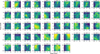 |
Fig. A.1 2D correlations across observations of the unsigned longitudinal magnetic field vs absolute RVs for the iron 6302.15 Å line for each of the forty seven pointings. Observation number and significance C for each observation is seen above each subfigure. |
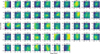 |
Fig. A.2 2D correlations across observations of the unsigned longitudinal magnetic field vs absolute RVs for the Ca 8542.09 Å line for each of the forty seven pointings. Calculations on the magnetic field and RVs were taken on the entire Ca line. Observation number and C for each observation is seen above each subfigure. |
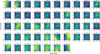 |
Fig. A.3 2D correlations across observations of the transversal magnetic field vs absolute RVs for the iron 6302.15 Å line for each of the forty seven pointings. Observation number and C for each observation is seen above each subfigure. |
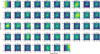 |
Fig. A.4 2D correlations across observations of the transversal magnetic field vs absolute RVs for the Ca 8542.09 Å line for each of the forty seven pointings. Calculations on the magnetic field and RVs were taken on the entire Ca line. Observation number and C for each observation is seen above each subfigure. |
All Figures
|
Fig. 1 Intensity map in Stokes I of all 47 observations. The mosaic is split into four parts for readability. Observations are taken from the western to eastern sides of the Sun. No merging images into a single mosaic using the overlap regions was attempted. To the upper right of each observation square is the μ value of each observation. All observations shown here come from the Stokes I observations of the Fe I 6301 Å line with a matched colour bar, with brighter colour showing more flux. |
| In the text | |
|
Fig. 2 Response function of the Fe lines (left) and the Ca line (right). The top shows the derivatives of the Stokes I relative to the gas temperature and the bottom shows the derivatives of the Stokes V relative to Bz. The synthetic profile is over-plotted in blue. |
| In the text | |
|
Fig. 3 Averaged correlations between the RVs and either the longitudinal or transversal magnetic fields derived from the Fe I 6302.15 and Ca II 8542 Å lines. The active averages were taken from observations 23, 35, and 36. The quiescent averages were taken from all remaining observations except for observations 0 and 46. |
| In the text | |
|
Fig. 4 Fragment of intensity image from observation 25 corresponding to the quiescent region of the photosphere close to the disc centre. Over-plotted are the contours of the absolute values of RV (top), longitudinal magnetic field (middle), and transversal magnetic field (bottom). Darker contours correspond to higher values. |
| In the text | |
|
Fig. 5 Computed values of RV, Bz, and Bt when observations are binned into one data point. Similar to the 2D case, absolute values are taken of the radial velocities and Bz. Observations 23, 35, and 36 contain magnetically active regions. |
| In the text | |
|
Fig. 6 Correlations of radial velocities derived from the three individual lines against magnetic field components Bz and Bt, when each observation has been binned to a single data point in Stokes IQUV. Observations are correlated against each other, and correlation values normalized. |
| In the text | |
|
Fig. 7 Comparisons of the correlations of the longitudinal magnetic field to the RVs derived from the Ca II 8542 Å line. The RVs were calculated using either the entire line profile (left column), the core of the line (|Δλ| < 0.3 Å, middle column), or just the wings (|Δλ| > 0.3 Å, right column). All figures are based on the 28th pointing. |
| In the text | |
|
Fig. 8 Magnetic field strength |B|, and the source function fit coefficients S0 and S1 (top row) and their correlations to the absolute value of RVs (middle row). 1D slices taken through the middle of the 2D correlation plots portray the relative correlation strengths (bottom row). All figures are based on the 33rd pointing. |
| In the text | |
|
Fig. A.1 2D correlations across observations of the unsigned longitudinal magnetic field vs absolute RVs for the iron 6302.15 Å line for each of the forty seven pointings. Observation number and significance C for each observation is seen above each subfigure. |
| In the text | |
|
Fig. A.2 2D correlations across observations of the unsigned longitudinal magnetic field vs absolute RVs for the Ca 8542.09 Å line for each of the forty seven pointings. Calculations on the magnetic field and RVs were taken on the entire Ca line. Observation number and C for each observation is seen above each subfigure. |
| In the text | |
|
Fig. A.3 2D correlations across observations of the transversal magnetic field vs absolute RVs for the iron 6302.15 Å line for each of the forty seven pointings. Observation number and C for each observation is seen above each subfigure. |
| In the text | |
|
Fig. A.4 2D correlations across observations of the transversal magnetic field vs absolute RVs for the Ca 8542.09 Å line for each of the forty seven pointings. Calculations on the magnetic field and RVs were taken on the entire Ca line. Observation number and C for each observation is seen above each subfigure. |
| In the text | |
Current usage metrics show cumulative count of Article Views (full-text article views including HTML views, PDF and ePub downloads, according to the available data) and Abstracts Views on Vision4Press platform.
Data correspond to usage on the plateform after 2015. The current usage metrics is available 48-96 hours after online publication and is updated daily on week days.
Initial download of the metrics may take a while.