© The Authors 2026

1 Introduction

The orbital and rotational evolution of natural satellites is strongly influenced by tidal dissipation processes, which play a key role in determining their internal structure, thermal state, and the presence of subsurface oceans, as is spectacularly observed in Europa and Enceladus. Tidal effects arise when an external perturbing body interacts gravitationally with an extended body. The gradient of the external gravitational field creates a differential gravitational attraction across the satellite, leading to physical deformation, mass redistribution, and variations in its gravitational field (Murray & Dermott 1999). For a satellite in an eccentric orbit and in synchronous rotation, the changing distance from its host planet causes the size and orientation of this tidal bulge to constantly change. According to classical tidal theory, these periodic deformations cause dissipation within the satellite’s interior due to frictional damping of the equilibrium tide (Kaula 1964). Other theories propose that, under certain conditions, the natural frequency of the normal modes of a subsurface ocean can approach the diurnal tidal frequency, which could lead to a resonant amplification of tidal dissipation (Hay et al. 2022).

One of the main methods of quantifying tidal dissipation in a body consists in detecting the tidal variation of gravity via radio tracking of spacecraft across multiple flybys or during an orbital phase. For example, this has been possible for the Moon with the GRAIL mission (Konopliv et al. 2013; Williams & Boggs 2015), and it will likely be possible in the future for Ganymede and Europa, due to the large quantity of high-quality data that JUICE and Europa Clipper will provide (Cappuccio et al. 2020; Mazarico et al. 2023; Magnanini et al. 2024).

Another method, more common in present-day literature, quantifies the characteristic secular orbital evolution of moons induced by tidal interactions (as detailed in the following sections) with astrometric observations from Earth or spacecraft and spacecraft radio science data (Lainey et al. 2009; Jacobson 2022). However, the orbital evolution is governed by tides on both the central body and the satellites, with similar signatures on the satellites’ orbits, making it challenging to distinguish their contributions using orbital data alone. Combining orbital tracking with direct gravity measurements from spacecraft flybys can help break this correlation (Magnanini et al. 2024). Therefore, it is important to have consistent tidal models in the dynamics of the moons and the spacecraft.

The effects of tides on the dynamics of moons have been widely studied. In this work, we focus on the orbital effect due to tides raised by the central planet on moons in synchronous rotation, as has been studied in many works such as Segatz et al. (1988), Yoder & Peale (1981), Murray & Dermott (1999), Boué & Efroimsky (2019) and Emelyanov (2018). Synchronous rotation is very common among the major moons in the Solar System, as it represents the minimum energy state resulting from dissipative phenomena, driven by interactions with the central planet (Murray & Dermott 1999). An introduction to the typical modeling approaches adopted in literature will be presented in Section 2.2. However, there are discrepancies in the literature regarding the effect of tidal dissipation on the long-term evolution of moons in synchronous rotation.

The first predictions of the energy dissipation due to tides within a satellite in synchronous rotation were obtained by employing what we call an “energetic method” (Segatz et al. 1988; Yoder & Peale 1981; Murray & Dermott 1999). The derived results have been the basis for several works on tides; for example, Tobie et al. (2005), Lainey et al. (2012), and Downey & Nimmo (2025). As was explained in Murray & Dermott (1999), assuming a satellite in Keplerian orbit around the planet and in perfectly synchronous rotation (see Section 2.2), the degree-2 tidal potential generated by the planet on the moon can be decomposed into two main components: the radial tide, caused by the variation in the moon’s orbital distance along its eccentric path, and the librational tide, which arises because the satellite does not always point to the planet, causing the tidal bulge to oscillate across its surface. By computing the stress and strain induced by the tidal cycle, and assuming that the energy dissipation from radial and librational tides can be linearly summed, we obtained the total energy dissipation in the satellite: $$\frac{dE}{dt}=-\frac{21}{2}\frac{k_2}{Q}\frac{R^{5}G{M}_p^{2}n}{a^6}{e}^2,$$(1) where G is the gravitational constant, M_p is the planet’s mass, R the reference radius of the satellite, and n and a are the mean motion and semimajor axis of the satellite’s orbit, respectively. k₂ is the degree-2 Love number, which quantifies the elastic response of the satellite to the tidal potential, and Q is the quality factor, representing the efficiency of energy dissipation, as is explained in Section 2.1.

Eq. (1) was derived under the assumption of no physical librations, implying that the satellite’s spin rate is strictly equal to its mean motion. Under this assumption the rotational energy cannot be diminished (Yoder & Peale 1981); consequently, any tidal energy dissipated due to a nonzero eccentricity must be drawn solely from its orbital energy (Murray & Dermott 1999).

From the classical orbital mechanics expression of the orbital energy (Murray & Dermott 1999), $$E=-\frac{G{M}_{p}m}{2a},$$(2) we can obtain a link between the variations of the orbital energy and the semimajor axis, $$\frac{dE}{dt}=\frac{G{M}_{p}m}{2a^2}\frac{da}{dt},$$(3) where m is the mass of the satellite. From orbital angular momentum conservation, the eccentricity rate can be linked to the semimajor axis rate. The square of the specific orbital angular momentum is defined as $$h^2={\mu }_{p}a(1-e^2),$$(4) where μ_p=GM_p is the gravitational parameter of the central body. Then, imposing the derivative to be 0, $$\frac{d{h}^2}{dt}={\mu }_p\frac{da}{dt}(1-e^2)-2{\mu }_{p}ae\frac{de}{dt}=0,$$(5) which yields to $$\frac{de}{dt}=\frac{(1-e^2)}{2ae}\frac{da}{dt}.$$(6)

Eqs. (1), (3), and (6) lead to the expressions for the tidal evolution of the orbital parameters, which were also reported for example in Lainey et al. (2012): $${\langle \frac{da}{dt}\rangle }_{EN}=-21\frac{{\mu }_p}{\mu }{\left(\frac{R}{a}\right)}^5\frac{k_2}{Q}na{e}^2,$$(7) $${\langle \frac{de}{dt}\rangle }_{EN}=-\frac{21}{2}\frac{{\mu }_p}{\mu }{\left(\frac{R}{a}\right)}^5\frac{k_2}{Q}ne,$$(8) where the subscript EN stands for energetic method. Eqs. (7) and (8) describe how the tides exerted by the planet on the satellite lead to orbital circularization and reduction of the semimajor axis, until the orbit eventually becomes circular and tidal dissipation stops.

Therefore, the amount of tidal dissipation in terms of the parameter $\frac{k_2}{Q}$ can be derived from the orbital evolution. However, more recent studies employing alternative approaches have yielded different results. In particular, methods based on the variation in orbital elements, the Lagrange planetary equations (Murray & Dermott 1999), as implemented independently by Boué & Efroimsky (2019) and Emelyanov (2018), indicate a significantly different orbital evolution coefficient for the semimajor axis, where the coefficient 57 appears instead of 21 given by Eq. (7). Since the semimajor axis variation is directly linked to tidal energy dissipation, this discrepancy, by roughly a factor of three, can introduce biases of a similar magnitude when deriving dissipation parameters from observational data.

In this work, we aim to understand the origin of this difference and provide a consistent way of estimating tidal dissipation of satellites in synchronous rotation, from both their orbital drifts and gravity measurements. In this context, tidal dissipation is typically modeled using two main approaches: the time-lag (TL) model introduced by Mignard (1979) and widely adopted in studies such as Lainey et al. (2009) and Jacobson (2022), where dissipation is represented through a time delay in the gravitational response of the satellite to the perturbing potential; and the complex Love number (CLN) model, described by Petit & Luzum (2010) and used in works such as Williams & Boggs (2015) and Cappuccio et al. (2020), which models dissipation by defining the Love number as a complex number whose phase lag is proportional to the energy loss. A complete mathematical description of these models is provided in Section 2.1.

Recent studies suggest that a frequency-dependent formulation may provide a more realistic representation of tidal dissipation, linking it to the body’s rheology (Efroimsky & Makarov 2013). In the frequency-dependent approach, the tidal perturbation is decomposed into a Fourier series, where each term is characterized by a specific lag (Efroimsky & Makarov 2013).

However, these models would require an increasingly high number of parameters the more complex the orbital dynamics becomes. This makes estimating dissipative parameters impractical, given that available data has so far only been sufficient to measure dissipation at the orbital period (Lainey et al. 2009; Park et al. 2021, 2025). Indeed, our primary interest is in tidal dissipation models that can be reliably used to reconstruct spacecraft and moon trajectories from observational data. The TL and CLN models remain the most widely used approaches for this purpose and can provide an estimation of the total internal dissipation in the bodies, even if without distinguishing between contributions from different frequency modes for each perturbing body.

In the current literature, there exist formulas that may establish a connection between the TL model and the CLN model, as is discussed in Section 2.1. However, to our knowledge, the dynamical effects of these two models have never been systematically analyzed, making it unreliable to compare the results obtained using different dissipation models.

This paper is organized as follows. Section 2 introduces the two tidal dissipation models used in this study, TL and CLN, and reviews the classical synchronous rotation model. In Section 3, we analyze the orbital evolutions predicted by these two approaches, comparing their results with each other and with findings from the literature. We then investigate the source of any resulting discrepancies. Section 4 discusses the implications of our work, and finally Section 5 summarizes our main conclusions.

2 Theoretical framework

2.1 Tidal models for gas giants’ satellite ephemerides

The static gravity potential of a non-spherically symmetric body can be expressed using a spherical harmonic expansion: $$\mathcal{U}(r,\varphi ,\lambda )=-\frac{\mu }{r}{\displaystyle \sum _{l=0}^{\infty }}{\displaystyle \sum _{m=0}^l}{\left(\frac{R}{r}\right)}^l{\overline{P}}_{l,m}(sin\varphi )[{\overline{C}}_{l,m}cosm\lambda +{\overline{S}}_{l,m}sinm\lambda ],$$(9) where μ=GM is the gravitational parameter of the body, R is the reference radius, r, φ, and λ are the body-fixed radial distance, latitude, and longitude of the point where the potential is to be evaluated, respectively, P̄_{l, m} is the fully normalized associated Legendre function of degree l and order m, and C̄_{l, m} and S̄_{l, m} are the fully normalized spherical harmonic coefficients.

An external body, p, with gravitational parameter μ_p produces a tidal potential, W, on the extended body, modifying its shape-mass distribution, and so its gravitational potential. The tidal potential on the surface of the perturbed body is (Efroimsky & Williams 2009) $$W(\mathbf{R},{\mathbf{r}}_{\mathbf{p}})=-\frac{{\mu }_p}{r_p}{\displaystyle \sum _{l=2}^{\infty }}{\left(\frac{R}{r_p}\right)}^l{P}_l(cosS),$$(10) where r_p is the position of the perturber with respect to the tidal body, R is the position vector of a point on the surface, and $S=arccos\left(\frac{\mathbf{R}·{\mathbf{r}}_{\mathbf{p}}}{R{r}_p}\right)$ is the angle between R and r_p. Exploiting the addition theorem for spherical harmonics the tidal potential can be written in terms of body-fixed coordinates: $$\begin{array}{rr}W(\mathbf{R},{\mathbf{r}}_{\mathbf{p}})=\hfill & -\frac{{\mu }_p}{r_p}{\displaystyle \sum _{l=2}^{\mathrm{\infty }}}{\left(\frac{R}{r_p}\right)}^l{\displaystyle \sum _{m=0}^l}{\overline{P}}_{l,m}(\sin \varphi )\hfill \\ & \times {\overline{P}}_{l,m}(\sin {\varphi }_p)[\cos (m\lambda )\cos \left(m{\lambda }_p\right)\hfill \\ & +\sin (m\lambda )\sin \left(m{\lambda }_p\right)]\hfill \\ \hfill & =-\frac{{\mu }_p}{r_p}{\displaystyle \sum _{l=2}^{\mathrm{\infty }}}{\left(\frac{R}{r_p}\right)}^l{\displaystyle \sum _{m=0}^l}{W}_{l,m}(\hat{\mathbf{R}},\widehat{{\mathbf{r}}_{\mathbf{p}}}).\hfill \end{array}$$(11)

In the equilibrium tides approximation, and assuming linear deformations, the gravity potential variation, Δ𝒰, on the surface can be expressed to be linearly proportional to the tidal potential through the so-called Love numbers, k_{l, m} (Kaula 1964): $$\Delta \mathcal{U}(\mathbf{R},{\mathbf{r}}_{\mathbf{p}})=-\frac{{\mu }_p}{r_p}{\displaystyle \sum _{l=2}^{\infty }}{\left(\frac{R}{r_p}\right)}^l{\displaystyle \sum _{m=0}^l}{k}_{l,m}{W}_{l,m}(\widehat{\mathbf{R}},\widehat{{\mathbf{r}}_{\mathbf{p}}}).$$(12)

Then, the potential variation, Δ𝒰, at a point, r, outside the body decreases as r^−(l+1): $$\Delta \mathcal{U}(\mathbf{r},{\mathbf{r}}_{\mathbf{p}})=-\frac{{\mu }_p}{r_p}{\displaystyle \sum _{l=2}^{\infty }}{\left(\frac{R}{r_p}\right)}^l{\left(\frac{R}{r}\right)}^{l+1}{\displaystyle \sum _{m=0}^l}{k}_{l,m}{W}_{l,m}(\widehat{\mathbf{R}},\widehat{{\mathbf{r}}_{\mathbf{p}}}).$$(13)

For a non-perfectly elastic body, we can use the vector position of the perturber, seen by the body-fixed reference frame of the tide body, corrected for the lag of the tidal bulge ${\mathbf{r}}_{\mathbf{p}}^{*}$: $$\Delta \mathcal{U}(\mathbf{r},{\mathbf{r}}_{\mathbf{p}}^{*})=-\frac{{\mu }_p}{r_p^{*}}{\displaystyle \sum _{l=2}^{\infty }}{\left(\frac{R}{r_p^{*}}\right)}^l{\left(\frac{R}{r}\right)}^{l+1}{\displaystyle \sum _{m=0}^l}{k}_{l,m}{W}_{l,m}(\widehat{\mathbf{R}},{\widehat{\mathbf{r}}}_{\mathbf{p}}^{*}).$$(14)

Finally, combining Eqs. (14) and (13), the potential variation due to tides can be written in terms of time-varying corrections to the spherical harmonics coefficients of the central body. In particular, considering only the degree-2 terms, which are dominant: $$\Delta {\overline{C}}_{2,m}-i\Delta {\overline{S}}_{2,m}=\frac{k_{2,m}}{5}\frac{{\mu }_p}{\mu }{\left(\frac{R}{r_p^{*}}\right)}^3{\overline{P}}_{2,m}(sin{\varphi }_p^{*})e^{-im{\lambda }_p^{*}},$$(15) where the delta-gravity coefficients are expressed normalized, $r_p^{*},{\varphi }_p^{*}$, and ${\lambda }_p^{*}$, are, respectively, the radial position, latitude, and longitude of the perturbing body seen in the body-fixed reference frame of the tide body, corrected for the lag of the tidal bulge, μ is the gravitation parameter of the tide body, and P̄_{2, m} is the associated normalized Legendre polynomial.

A common approach to express the tidal dissipation is to evaluate the position of the perturber in the body-fixed reference frame of the tide body with a time delay, Δ t, i.e., ${\mathbf{r}}_{\mathbf{p}}^{*}\left(t\right)={\mathbf{r}}_{\mathbf{p}}(t-\Delta t)$ (Mignard 1979). Δ t effectively represents the delay at which the body reacts to the external tidal potential. This model is commonly referred as the TL model, as was outlined in Section 1.

Note that usually in the literature it is implicitly assumed that the Love numbers are the same at all the orders, i.e., k₂=k_2,0= k_2,1=k_2,2 (Mignard 1979; Lainey et al. 2009; Jacobson 2022), and in this work we also follow this assumption. Some studies consider several modes with different constants, k_{2, m} (e.g., Park et al. 2021), which, while theoretically expected to be very similar, have been observed to differ slightly for the Earth-Moon system due to the exceptional quality and quantity of available data.

In most of the works, the tidal dissipation of celestial bodies is quantified by a parameter, Q, called the “quality factor,” which comes from an analogy to a damped oscillator, and defined as the ratio between the energy of the system and the energy lost per radian during the period (Murray & Dermott 1999): $$Q=-2\pi \frac{E_{peak}}{\mathrm{\Delta }{E}_{diss}},$$(16) where E_peak and Δ E_diss are the peak energy stored and the energy dissipated during one period, respectively.

The quality factor has been related to the TL through the phase-lag, ε, associated with the delay of the perturber, seen in the body-fixed frame of the tide body. For example in Efroimsky & Makarov (2013) this relationship is $$sin\left(ϵ\right)=\frac{1}{Q}.$$(17)

The connection between Q and Δ t is (supplementary information of Lainey et al. 2009) $$sin\left(2\pi \frac{\Delta t}{\tau }\right)=\frac{1}{Q},$$(18) where τ is the period of the main tidal excitation as seen in the body-fixed frame. For the tides raised by the central planet on a synchronous satellite: $$\tau =\frac{2\pi }{n}=T,$$(19) where T and n are the orbital period and the mean motion of the satellite, respectively. Therefore, the relationship between the phase-lag and the TL for satellites in synchronous rotation can be written as $$ϵ=n\Delta t.$$(20)

Notably, in the literature the TL model has been implemented following different physical assumptions. Some studies, such as Lainey et al. (2009), adopt a constant quality factor, Q. This results in a constant phase lag, which is not generally equivalent to a constant time lag. Conversely, other works, such as Jacobson (2022), assume a constant time lag, which in turn does not generally imply a constant phase lag.

However, importantly, both approaches model tidal dissipation by considering the tidal bulge to point not at the perturber’s instantaneous position, r, but toward a lagged position along its orbit, r^*(v−Δ v) (where v is the true anomaly of the satellite). This orbital lag, whether defined as a time delay or a corresponding phase angle, consequently influences all spherical coordinates used to define the perturber’s position.

Another commonly used approach to model the tidal dissipation is to use CLNs (Eanes et al. 1983; Petit & Luzum 2010; Williams & Boggs 2015; Cappuccio et al. 2020; Mazarico et al. 2023): $$\Delta \mathcal{U}(\mathbf{r},{\mathbf{r}}_{\mathbf{p}})=-\frac{{\mu }_p}{r_p}{\displaystyle \sum _{l=2}^{\infty }}{\left(\frac{R}{r_p}\right)}^l{\left(\frac{R}{r}\right)}^{l+1}{\displaystyle \sum _{m=0}^l}{k}_{l,m}^c{W}_{l,m}(\mathbf{r},{\mathbf{r}}_{\mathbf{p}}),$$(21) where now ${\mathbf{r}}_{\mathbf{p}}^{*}\left(t\right)={\mathbf{r}}_{\mathbf{p}}\left(t\right)$ and $k_{l,m}^c$ is the CLN with modulus k_{l, m} and phase ϕ_l,m, $$k_{l,m}^c=\Re \left(k_{l,m}^c\right)+i\mathfrak{I}\left(k_{l,m}^c\right)=k_{l,m}(cos{\phi }_{l,m}+isin{\phi }_{l,m}).$$(22)

Writing in terms of gravity coefficients, Eq. (21) now becomes $$\Delta {\overline{C}}_{2,m}-i\Delta {\overline{S}}_{2,m}=\frac{k_{2,m}}{5}\frac{{\mu }_p}{\mu }{\left(\frac{R}{r_p}\right)}^3{\overline{P}}_{2,m}(sin{\varphi }_p)e^{-i(m{\lambda }_p-{\phi }_{2,m})}.$$(23)

Effectively, the phase of the Love numbers modifies the body-fixed longitude of the perturber, as for a rotation around the Z-axis of the body-fixed frame by the lag angle Δ λ_{2, m}=ϕ_{2, m}/m. In this model, the real part, 𝕽(k_l,m), characterizes the instantaneous in-phase (elastic) response, while the imaginary part, 𝕵(k_l,m), characterizes the out-of-phase (dissipative) response. As was outlined in Section 1, we refer to this model as the CLN model.

It is important to note that the phase of the Love number, which represents the offset of the tidal bulge, and so the dissipation, modifies only the body-fixed longitude of the perturber, while it does not affect the radial distance. In other words, the CLN model does not consider the position of the perturber at some point in the past along its orbit, but it only rotates the tidal bulge around the spin axis by an angle, Δ λ, proportional to the phase of the CLN. Moreover, the lag angle is also explicitly a function of the order m, so the classical assumption $k_2^c=k_{2,0}^c=k_{2,1}^c=k_{2,2}^c$ leads to different lag angles between order 1 and order 2, i.e., Δ λ_2,1=ϕ_2,1 and Δ λ_2,2=ϕ_2,2/2. Hence, in the CLN model, to have the same tidal response for all orders, both elastic and dissipative, the following conditions must be imposed: $$k_{l,m}=k_l$$(24) and $${\phi }_{l,m}=m{\phi }_l.$$(25) However, most of the natural satellites of the outer planets are in spin-orbit resonance, with small obliquities, so that the inclination of the central planet in the body-fixed frame is very small, making the tidal contribution of the (l,m)=(2,1) coefficients negligible with respect to the (l,m)=(2,2) terms. Possible exceptions may be the Moon and Triton, where the obliquity tides may play a crucial role in present-day heat production and internal structure.

For the CLN model, in the literature the connection between $\mathfrak{J}\left(k_2^c\right)$ and Q for satellites in synchronous rotation has been written as (Segatz et al. 1988; Efroimsky & Makarov 2013)¹ $$\mathfrak{J}\left(k_2^c\right)=\frac{k_2}{Q},$$(26) where this time the phase lag of the CLN is associated with Q: $$sin\left({\phi }_2\right)=\frac{1}{Q}.$$(27)

Therefore, in the literature, the TL and CLN models for satellites in synchronous rotation are commonly related through (Efroimsky & Makarov 2013) $$\frac{k_2}{Q}=\mathfrak{I}\left(k_2^c\right)=k_{2}sin\left(n\Delta t\right).$$(28)

However, there is a fundamental conceptual difference between the two models in their physical approximation of the tidal lag. The TL model considers the tidal bulge to be directed toward a past position of the perturber along its orbit. This method inherently incorporates the corresponding change in radial distance. In contrast, the CLN model applies the lag as a pure angular rotation of the tidal bulge and does not alter the instantaneous distance to the perturber. Consequently, the phase lag derived from the TL model and the phase of the CLN cannot be considered physically equivalent.

Depending on the orbit of the body and its rotational state, Δ C̄_{2, m} and Δ S̄_{2, m}, computed from the tidal models described above may have a nonzero average over the orbital period, usually called “permanent tide,” which becomes by all means part of the static gravity potential. Hence, to compute the effective tidal effects, the permanent tide must be removed from the coefficient corrections given by Eqs. (15) and (23), obtaining the purely periodic tidal corrections: $$\mathrm{\Delta }{\overline{C}}_{2,m}^{periodic}=\mathrm{\Delta }{\overline{C}}_{2,m}-⟨\mathrm{\Delta }{\overline{C}}_{2,m}⟩$$(29) and $$\mathrm{\Delta }{\overline{S}}_{2,m}^{periodic}=\mathrm{\Delta }{\overline{S}}_{2,m}-⟨\mathrm{\Delta }{\overline{S}}_{2,m}⟩.$$(30)

Note that $\mathrm{\Delta }{\overline{C}}_{2,m}^{periodic}$ and $\mathrm{\Delta }{\overline{S}}_{2,m}^{periodic}$ correspond to the “zero tide” tidal corrections, defined by the latest IERS conventions (Petit & Luzum 2010). Instead, 〈Δ C̄_{2, m}〉 and 〈Δ S̄_{2, m}〉 represent the permanent parts of Δ C̄_{2, m} and Δ S̄_{2, m}. The expressions and the full derivation of the degree-2 permanent tide terms for a satellite in spin-orbit resonance, for both the TL and the CLN models, are provided in Appendix A.

The gravitational interaction between an external point-mass and the figure of an extended body, represented by the nonzero degree terms of its potential given by Eq. (9), produces an acceleration on the body itself, which we call “self-figure,” given by (Park et al. 2021) $$\mathbf{f}=\left(\frac{{\mu }_p}{\mu }\right)\nabla \mathcal{U}.$$(31)

Then, regardless of the dissipation model considered, the tides exerted by the external point-mass perturber on the central body cause a variation of its gravity potential, and so a variation of the self-figure acceleration: $$\Delta \mathbf{f}=\left(\frac{{\mu }_p}{\mu }\right)\nabla \left(\Delta \mathcal{U}\right).$$(32)

The gradient must be evaluated in the body-fixed frame of the central body; thus, the gravitational acceleration must be rotated into the inertial frame to perform the integration. Hence, particular care must be taken in the modeling of the rotational state. In this work we neglect the torque coming from the figure-to-figure interaction, which, for natural satellites around gas giants, would have an effect beyond the fourth order in eccentricity, and so it can be considered negligible with respect to the self-figure induced acceleration.

2.2 Rotational model

Most of the natural satellites of the Solar System are assumed to be in synchronous rotation, also called spin-orbit resonance, meaning that the orbital and rotational periods are the same and the spin axis is perpendicular to the orbital plane (the so-called spin–orbit resonance, see e.g., Murray & Dermott 1999). In this state, the permanent bulge would ideally always point to the empty focus of the orbit, to the first order in eccentricity, oscillating around the direction of the central planet (optical libration). Furthermore, the misalignment between the permanent bulge and the central planet induces a periodic gravitational torque that produces an additional oscillation around the mean rotation (forced physical librations) (Van Hoolst et al. 2020). Because of other minor effects, such as third-body perturbations and internal dissipation, the forced librations are expected to be the combination of multiple oscillations at different frequencies, and resonances at frequencies of internal modes may occur (Rambaux et al. 2011).

Moreover, the spin axis is characterized by its tilt relative to the orbital plane (obliquity) and by its precise orientation in space. Determining these rotational parameters, alongside physical librations, offers crucial insights into a satellite’s interior (Hemingway & Nimmo 2024). For instance, the departure of the spin axis from its expected equilibrium state (the Cassini plane offset) was used to infer the tidal dissipation of Titan by Downey & Nimmo (2025).

The rotational and orbital dynamics are strongly coupled, as the self-figure acceleration of a satellite influences its orbit, and, at the same time, its rotational modes are forced by the dynamical interactions with the other bodies. Therefore, in principle, the set of equations governing translational and rotational dynamics should be coherently integrated, as was performed for the Moon in the planetary ephemerides (Folkner et al. 2014). This would ensure that the two dynamics are consistent. However, in numerous studies analyzing astrometric and radio tracking data from missions such as Cassini, Galileo, and Juno, a common approach has been to estimate the moons’ gravity fields under the assumption of synchronous rotation, occasionally including the libration at the orbital period (e.g., Lainey et al. 2019; Park et al. 2025). This assumption arises primarily because of the limited precision of available data and the lack of detailed direct observations of the moons’ rotational states.

Following Lainey et al. (2019), a possible approach to model the orientation of the satellites is the following: each time the spin axis, ẑ, is oriented as the instantaneous orbital angular momentum vector, i.e., $$\widehat{\mathbf{z}}=\frac{\mathbf{r}\times \mathbf{v}}{|\mathbf{r}\times \mathbf{v}|},$$(33) where r and v are the position and velocity of the satellite with respect to the planet, respectively. Then, the prime meridian, x̂, is computed from the direction of the central planet through a rotation around ẑ by an angle, λ: $$\lambda =-2e\sin M-\frac{5}{4}{e}^{2}sin(2M)+A\sin M,$$(34) where e and M are the instantaneous eccentricity and mean anomaly, respectively, and A is the amplitude of the main physical forced libration.

In this way, the rotational dynamics is imposed from the orbital motion. With this model, when A=0 the prime meridian always points to the empty focus of the orbit, at the first order in eccentricity (Murray & Dermott 1999). When A ≠ 0, the prime meridian oscillates periodically such that it consistently points farther from Jupiter than the direction of the empty focus, as is explained in Van Hoolst et al. (2020). Therefore, in Eq. (34) the libration amplitude should always be negative. Other physical libration terms at frequencies different from the orbital period are not expected to have a significant effect on the orbit (Rambaux et al. 2011), considering the sensitivity of past, current, and near-future data, and have been commonly neglected during data analysis.

This study assumes the rotational model defined by Eqs. (33) and (34), which is the standard reference for the data analyses and analytical works discussed in subsequent sections. In this work we refer to it as the “classical synchronous rotation” model. Our primary aim is to resolve a discrepancy in the literature concerning eccentricity effects, considering also the libration at the orbital period. To this end, the orbital influence of obliquity is neglected, with its contribution deferred to a future work.

3 Tidal orbital evolution of synchronous satellites

3.1 Gauss planetary equations

To study the effect of tidal dissipation on the eccentricity and semimajor axis, and therefore on the orbital energy, a more practical approach with respect to the energetic method, described in Sect. 1, is to apply the Gauss planetary equations (Battin 1999) that directly connect the tidal and rotational models to the variation of the orbital parameters. In this section only a brief summary of the procedure and the main results are provided, while the complete mathematical derivation is reported in Appendix A.

Following the same assumptions as in Segatz et al. (1988), Boué & Efroimsky (2019), and Emelyanov (2018), namely Keplerian orbit, synchronous rotation, zero libration amplitude, and zero obliquity, the spherical coordinates of the planet in the satellite’s body-fixed frame are computed at each point of the orbit, as a function of the mean anomaly. Then, the tidal variation in the gravity potential coefficients can be computed from Eqs. (15) and (23) for the CLN model and the TL model, respectively. The permanent tide can be computed averaging over the orbital period, and removed to obtain the purely periodic part of the tidal variations. Then, the corresponding acceleration in the body-fixed frame is computed from Eq. (A.29), and rotated in the RTN orbital frame, so that the time derivative of the orbital parameters can be computed directly through the Gauss planetary equations. Finally, the secular orbital effects are computed averaging these derivatives over the orbital period. All the computations in this work use a second-order approximation in eccentricity.

To validate this analytical procedure, the resulting expressions were compared with numerical integrations of the full equations of motion using MONTE software (Evans et al. 2018). This comparison showed full agreement in the secular variation of the orbital elements.

In the following sections, the results are reported for both the tidal models. Note that, because of their importance, only the semimajor axis and eccentricity are reported in this work, but the same process can be applied for all the orbital elements.

3.1.1 Complex Love number model

As is derived in Appendix A.4, the secular variations of the semimajor axis and the eccentricity for the CLN model result in $${\langle ;\frac{da}{dt}\rangle }_{CLN}=-55.5\frac{{\mu }_p}{\mu }{\left(\frac{R}{a}\right)}^5\mathfrak{J}\left(k_{2,2}^c\right)na{e}^2$$(35) and $${\langle \frac{de}{dt}\rangle }_{CLN}=-9\frac{{\mu }_p}{\mu }{\left(\frac{R}{a}\right)}^5\mathfrak{I}\left(k_{2,2}^c\right)ne.$$(36)

However, as was outlined in Section 1, neither Eq. (35) nor Eq. (36) agrees with the expressions resulting from the energetic methods of Segatz et al. (1988) and Yoder & Peale (1981).

In particular, for the semimajor axis, the energetic method obtains a coefficient 21, while the direct approach obtains 55.5, almost a factor of 3 larger. As the semimajor axis evolution is directly related to energy dissipation, this means that we find tidal dissipation a factor of ≈ 3 larger, under the same assumptions for the orbit and rotation. For the eccentricity, the difference is smaller: a coefficient of 10.5 appears in the results of the energetic method, against 9 derived from the Gauss planetary equations.

3.1.2 Time-lag model

Following the same methodology as in the previous section, reported in detail in Appendix A.5, the secular trends of the semimajor axis and eccentricity for the TL model are found: $${\langle \frac{da}{dt}\rangle }_{TL}=-57\frac{{\mu }_p}{\mu }{\left(\frac{R}{a}\right)}^5{k}_{2}sin\left(n\Delta t\right)na{e}^2$$(37) and $${\langle \frac{de}{dt}\rangle }_{TL}=-\frac{21}{2}\frac{{\mu }_p}{\mu }{\left(\frac{R}{a}\right)}^5{k}_{2}sin\left(n\Delta t\right)ne.$$(38)

Looking at the numerical coefficients, considering $\frac{1}{Q}=sin\left(n\Delta t\right)$, the eccentricity rate is characterized by the coefficient 10.5, which matches the energetic method, while the semimajor axis has the coefficient 57, larger than the 21 of the energetic approach by almost a factor of 3.

However, our results 37 and 38 are in accordance with Eqs. (150) and (159) in Boué & Efroimsky (2019). In their work, an approach similar to the one described above was followed, as the Lagrange planetary equations were exploited to retrieve orbital element evolution from the tidal potential of the satellite and the central body, under the same assumptions. They considered a frequency-dependent Kaula model (Kaula 1964), but found that, in the case of a synchronous satellite, the expression for the secular change in the semimajor axis simplifies to depend on only one tidal mode, the mean motion, n. As a result, the expression becomes frequency-independent and equivalent to both constant phase-lag and constant TL assumptions Boué & Efroimsky (2019).

In summary, we find that both the TL and the CLN models produce an orbital evolution that does not match the results of the energetic method, with an energy dissipation increased by almost a factor of 3. In addition, TL and CLN do not produce the same orbital evolution, considering the relations between Δt and $\mathfrak{J}\left(k_{2,2}^c\right)$ available in current literature (Efroimsky & Makarov 2013, 2014).

3.2 Conservation of angular momentum

In Boué & Efroimsky (2019), in view of the result found, the −21 coefficient of the energy approach (used in Lainey et al. 2012) was considered to be a mistake. However, an important aspect is missing to compute with the current assumptions: the conservation of angular momentum.

In the purely elastic case, as was said before, the tidal bulge is always aligned toward the perturbing body and, because of symmetry, the resulting gravity torque is null. Consequently, there is no transfer of angular momentum between the two bodies. In the inelastic case, the bulge is offset with respect to the direction of the perturbing body by a certain lag, and the resulting tidal torque drives an exchange of angular momentum.

Assuming a point-mass planet and a non-spherical satellite in synchronous rotation without physical librations – implying that the satellite’s spin rate is strictly equal to the mean motion the total angular momentum vector with respect to the planet is given by Murray & Dermott (1999) $$\mathbf{L}=\mathbf{r}\times \mathbf{p}+\tilde{C}M{R}^{2}n\widehat{\mathbf{z}},$$(39) where p=M v is the linear momentum of the satellite, C̃ is the normalized polar moment of inertia, and M, R and n are the mass, radius, and mean motion of the satellite, respectively. The first term of the equation represents the orbital angular momentum, while the second represents the spin angular momentum. For a satellite in synchronous rotation, both terms are along the normal to the orbital plane, so we can only study the modulus of the angular momentum.

3.2.1 Time-lag model

Considering the TL tidal model, the secular variation of the orbital angular momentum, to the second order in eccentricity, can be derived as (for the detailed procedure, see Appendix B) $${⟨\frac{d{L}_{orb}}{dt}⟩}_{TL}=-18\frac{{\mu }_p^2}{R\mu }{\left(\frac{R}{a}\right)}^{6}M{k}_2\sin (n\mathrm{\Delta }t)e^2.$$(40)

Instead, for the spin angular momentum we find: $$\begin{array}{rl}{⟨\frac{d{L}_{spin}}{dt}⟩}_{TL}& =\frac{171}{2}\tilde{C}\frac{{\mu }_p^2}{R\mu }{\left(\frac{R}{a}\right)}^{6}M{k}_2\sin (n\mathrm{\Delta }t)e^2{\left(\frac{R}{a}\right)}^2\\ & ={⟨\frac{d{L}_{orb}}{dt}⟩}_{TL}4.75\tilde{C}{\left(\frac{R}{a}\right)}^2.\end{array}$$(41)

For the natural satellites of the outer planets, C̃ ≈ 0.3−0.4 (for example, Io’s C̃ ≈ 0.37−0.38 (Schubert et al. 2004)), while $\left(\frac{R}{a}\right)\ll 1$, so the secular variation of the spin angular momentum is negligible with respect to the orbital one, obtaining $${⟨\frac{dL}{dt}⟩}_{TL}\approx {⟨\frac{d{L}_{orb}}{dt}⟩}_{TL}=-18\frac{{\mu }_p^2}{R\mu }{\left(\frac{R}{a}\right)}^{6}M{k}_2\sin (n\mathrm{\Delta }t)e^2.$$(42)

Therefore, it is evident that the angular momentum is not conserved, highlighting the presence of mistakes in the assumptions.

Hence, we searched for conditions that may be able to conserve the total angular momentum. In particular, because of the tidal effects, all the satellites in synchronous rotation possess a relatively large static (secular) degree-2 gravity field. Using the same approach described above, we can compute the corresponding secular orbital evolution and the variation of the orbital angular momentum, obtaining (the full derivation is available in Appendices A.3 and B.3) $${\langle \frac{da}{dt}\rangle }_{ST}=12\sqrt{\frac{{\mu }_p}{a}}{\left(\frac{R}{a}\right)}^2{S}_{2,2}(1-\frac{5}{2}{e}^2)$$(43) and $${⟨\frac{d{L}_{orb}}{dt}⟩}_{ST}=6\frac{{\mu }_p}{R}{\left(\frac{R}{a}\right)}^3{S}_{2,2}(1-\frac{5}{2}{e}^2).$$(44)

Among the static degree-2 terms, S_2,2 is the only static parameter that has a secular effect on the semimajor axis (and so on the orbital energy) and on the angular momentum.

Therefore, for an extended satellite in synchronous rotation, the total secular variation of the angular momentum is given by both the static gravity field and the tidal dissipation: $${⟨\frac{dL}{dt}⟩}_{TL}\approx {⟨\frac{d{L}_{orb}}{dt}⟩}_{TL}+{⟨\frac{d{L}_{orb}}{dt}⟩}_{ST}.$$(45)

Imposing $\langle \frac{dL}{dt}\rangle =0$, we can find the value of S_2,2 that allows the conservation of the angular momentum: $${\left(S_{2,2}^{*}\right)}_{TL}=3\frac{{\mu }_p}{\mu }{\left(\frac{R}{a}\right)}^3{k}_{2}sin\left(n\Delta t\right)e^2.$$(46)

In a principal axis frame, S_2,2=0 by definition (Bertotti et al. 2012). A nonzero S_2,2 represents a (constant) offset, Δ λ, between the body-fixed frame and the principal axis frame around the ẑ axis. In particular, assuming small rotations with respect to the principal axis frame, it holds (Bertotti et al. 2012): $$S_{2,2}=-2C_{2,2}\Delta \lambda .$$(47)

Therefore, the offset angle, Δ λ^*, that conserves the angular momentum is given by $${\left(\Delta {\lambda }^{*}\right)}_{TL}=-\frac{3}{2}\frac{{\mu }_p}{\mu }{\left(\frac{R}{a}\right)}^3\frac{1}{C_{2,2}}{k}_{2}sin\left(n\Delta t\right)e^2.$$(48)

As a result, in the presence of tidal dissipation, a constant offset of the prime meridian of the principal axis body-fixed reference frame from the classical synchronous rotation is necessary to conserve the angular momentum.

Note that, [even in presence of this offset], the satellite is still in synchronous rotation, as the rotation period remains equal to the orbital period. The same rotation offset was found by Williams et al. (2001) in Eq. (34a) and Noyelles (2017) in Eq. (93), which provided an analytical solution for the rotational dynamics of a satellite in synchronous rotation considering tidal dissipation. This effect was first predicted by Greenberg & Weidenschilling (1984) and was discussed in more detail in Murray & Dermott (1999) and Ferraz-Mello et al. (2008). In Ferraz-Mello et al. (2008) the analysis was also expanded considering a fully liquid body, without a permanent figure. In this scenario, an offset of the reference frame would not produce any torque, and to conserve the angular momentum a super-synchronous rotation is needed, so that the torque due to tidal dissipation averages out to zero over the orbital period. In this study we focus on a solid body scenario, which could be considered the case for the majority of the moons, where the relaxation time scale is much larger than the spin period of the body. However, considering a body with a subsurface liquid layer, such as the liquid water oceans inside Europa and Ganymede, or a magma ocean inside Io, there could be a decoupling between the internal layers and the shell, possibly leading to different configurations to conserve angular momentum. Due to its high complexity, this scenario is not addressed in this work.

Interestingly, by implementing the static $S_{2,2}^{*}$ given by Eq. (46) or, equivalently, the angular offset Δ λ^* given by Eq. (48), not only is the angular momentum conserved, but also the secular variation of the semimajor axis and eccentricity now perfectly match the expressions found with the energy approach: $${\langle \frac{da}{dt}\rangle }_{TL}^{*}=-21\frac{{\mu }_p}{\mu }{\left(\frac{R}{a}\right)}^5{k}_{2}sin\left(n\Delta t\right)na{e}^2$$(49) and $${\langle \frac{de}{dt}\rangle }_{TL}^{*}=-\frac{21}{2}\frac{{\mu }_p}{\mu }{\left(\frac{R}{a}\right)}^5{k}_{2}sin\left(n\Delta t\right)ne.$$(50)

This shows how simply imposing synchronous rotation as considered by Boué & Efroimsky (2019) is not enough when integrating the satellite ephemerides in presence of dissipation to obtain a consistent orbital evolution, and therefore the energy tidal dissipation, Ė. Instead, it must be taken into account that rotation of a satellite is not negligibly influenced by tidal dissipation, imposing an angular offset of the minimum inertia axis as given by Eq. (48) or, equivalently, an S_2,2 as given by Eq. (46).

3.2.2 Complex Love number model

The same procedure outlined in the previous section can also be applied to the CLN model, obtaining similar results in terms of $S_{2,2}^{\ast }$ or Δ λ^* necessary to conserve the angular momentum: $${\left(S_{2,2}^{*}\right)}_{CLN}=\frac{25}{8}\frac{{\mu }_p}{\mu }{\left(\frac{R}{a}\right)}^3\mathfrak{J}\left(k_{2,2}^c\right)e^2$$(51) and $${\left(\Delta {\lambda }^{*}\right)}_{CLN}=-\frac{25}{16}\frac{{\mu }_p}{\mu }{\left(\frac{R}{a}\right)}^3\frac{1}{C_{2,2}}\mathfrak{J}\left(k_{2,2}^c\right)e^2.$$(52)

Also in Eq. (51), the S_2,2 result to be positive definite as $\mathfrak{J}\left(k_{2,2}^c\right)$ due to tidal dissipation must be positive.

However, implementing the static $S_{2,2}^{*}$ (or the angular offset Δ λ^*) allows one to conserve the angular momentum, but the secular evolution of the semimajor axis and eccentricity do not match the TL model results: $${\langle \frac{da}{dt}\rangle }_{CLN}^{*}=-18\frac{{\mu }_p}{\mu }{\left(\frac{R}{a}\right)}^5\mathfrak{J}\left(k_{2,2}^c\right)na{e}^2$$(53) and $${\langle \frac{de}{dt}\rangle }_{CLN}^{*}=-9\frac{{\mu }_p}{\mu }{\left(\frac{R}{a}\right)}^5\mathfrak{I}\left(k_{2,2}^c\right)ne.$$(54)

The TL model results would be replicated considering the relation $$\mathfrak{J}\left(k_{2,2}^c\right)=\frac{7}{6}{k}_{2}sin\left(n\Delta t\right),$$(55) unlike the relation proposed in the literature reported in Eq. (28) (Segatz et al. 1988; Efroimsky & Makarov 2013, 2014).

The quality factor, Q, is related to the energy dissipation by definition. In Eqs. (53) and (49), we found that the TL and CLN models yield different orbital evolutions and, consequently, different energy dissipation rates. This implies that the phase lags of the two models – which are conceptually distinct (see Section 2.1) – cannot both be related to a single, universal Q through the same simple relationship. In other words, the phase lag of the two models cannot be associated with the same Q by the relations in Eqs. (17), (27) and (28), as is done in the current literature.

3.3 Effect of the libration at the orbital period

The libration at the orbital period produces an additional dissipative effect, contributing to the secular orbital effect caused by the eccentricity. The same approach described in Section 3.2 and further detailed in Appendices A.3, A.4, and A.5 can be followed, considering Eq. (34) with a nonzero libration amplitude, A. Then, the static value of S_2,2 that conserves the angular momentum (see Appendix B), and the corresponding secular orbital evolution, can be found.

3.3.1 Time-lag model

For the TL model the following results are obtained: $${\left(S_{2,2}^{*}\right)}_{TL}=(3e^2-\frac{3}{2}Ae)\frac{{\mu }_p}{\mu }{\left(\frac{R}{a}\right)}^3{k}_{2}sin\left(n\Delta t\right).$$(56)

Implementing the static $S_{2,2}^{*}$ (or the angular offset Δ λ^*), the secular evolution of the semimajor axis and eccentricity become $${\langle \frac{da}{dt}\rangle }_{TL}^{*}=(-21e^2+6Ae)\frac{{\mu }_p}{\mu }{\left(\frac{R}{a}\right)}^5{k}_{2}sin\left(n\Delta t\right)na$$(57) and $${\langle \frac{de}{dt}\rangle }_{TL}^{*}=(-\frac{21}{2}e+3A)\frac{{\mu }_p}{\mu }{\left(\frac{R}{a}\right)}^5{k}_{2}sin\left(n\Delta t\right)n.$$(58)

This time, we do not find the same result as an energetic method. In particular, the tidal dissipation provided by Eq. (96) of Efroimsky (2018), converted to $\frac{da}{dt}$, and assuming zero obliquity, would correspond to coefficients (−21e² + 12Ae −3 A²). We notice a factor 2 difference for the coefficient multiplying Ae and an additional term, −3A², independent of eccentricity, absent in our Eq. (57). This discrepancy possibly arises because the energetic method calculates the total power dissipated (the sum of rotational and orbital energy rates of change). In contrast, our computation isolates the work done on the orbit, which is the sole driver of the semimajor axis evolution. As is shown in Eq. (49), our approach aligns with the energetic method only in the absence of the physical libration, where the rate of change in the total energy is identical to that of the orbital energy.

3.3.2 Complex Love number model

For the CLN model, the following results are obtained: $${\left(S_{2,2}^{*}\right)}_{CLN}=(\frac{25}{8}{e}^2-16Ae+4A^2)\frac{{\mu }_p}{\mu }{\left(\frac{R}{a}\right)}^3\mathfrak{J}\left(k_{2,2}^c\right).$$(59)

The semimajor axis and eccentricity secular variations, having implemented the correction offset, are $${\langle \frac{da}{dt}\rangle }_{CLN}^{*}=(-18e^2+\frac{9}{2}Ae)\frac{{\mu }_p}{\mu }{\left(\frac{R}{a}\right)}^5\mathfrak{J}\left(k_{2,2}^c\right)na$$(60) and $${\langle \frac{de}{dt}\rangle }_{CLN}^{*}=(-9e+\frac{9}{4}A)\frac{{\mu }_p}{\mu }{\left(\frac{R}{a}\right)}^5\mathfrak{J}\left(k_{2,2}^c\right)n.$$(61)

To reconcile the orbital effect of the CLN and TL tidal models, the following relation must be satisfied: $$\mathfrak{J}\left(k_{2,2}^c\right)=\frac{7e-2A}{6e-\frac{3}{2}A}{k}_{2}sin\left(n\Delta t\right).$$(62)

When the libration amplitude is zero, the coefficient in Eq. (62) reduces to $\frac{7}{6}$, consistent with Eq. (55). This shows a different orbital response of the two tidal models to the rotation.

4 Discussion

Due to the triaxiality of the moons, their rotational and translational dynamics are coupled, meaning that, in principle, they should be integrated together as is explained in Section 2.2. This would ensure consistency of the dynamical model and the conservation of angular momentum. However, due to the limited precision of available data and the lack of detailed observations of the moons’ rotational states, simplified rotational models derived from the orbital state are usually employed. A common choice is to assume synchronous rotation, with the x axis pointing to the empty focus of the orbit [at the first order], with the possible addition of the physical libration [at the orbital period] (Eq. (34)).

In this work, we found that, when internal dissipation occurs within the satellite, this simplified rotational model cannot be used to integrate the ephemerides of the moon, because it leads to an orbital propagation that does not conserve the total angular momentum. Moreover, the secular evolution does not match the theoretical predictions obtained by the energy approach, resulting in a tidal dissipation rate almost three times higher. Consequently, if the tidal dissipation of a satellite is estimated based on its orbital evolution, the moon’s dissipative tidal parameters (either 𝕵(k₂) or Δ t) could be underestimated by the same factor. To correct this, a constant angular offset of the permanent bulge is necessary to create a restoring torque, conserving the angular momentum and maintaining synchronous rotation (Greenberg & Weidenschilling 1984).

This rotational frame offset can be introduced also by considering the classical synchronous frame, adding a positive S_2,2 in the gravity field of the moon. In fact, S_2,2 is the only static degree-2 gravity parameter that induces a secular effect on the satellite’s orbit, as is shown by Eq. (43) and derived in Appendix A.3.

Therefore, for moons that reached spin-orbit resonance and in the absence of dissipation, considering the classical synchronous rotation model, a nonzero S_2,2 would lead to changes in the system’s orbital energy and angular momentum without any corresponding physical phenomena (e.g., stress and strain induced by varying tidal potential). In this case, it is critical to constrain S_2,2 to zero, to ensure that the orbital and angular momentum variations are physically meaningful.

Note that the prime meridian can be chosen arbitrarily. The common choice for a synchronous satellite is to define the frame from the orbit; for example, pointing the x-axis to the empty focus, as is considered in this work. Another possibility could be to define the longitude of a specific feature on the surface (Park et al. 2024).

In this case, the values of the static gravity or the rotation offset that ensure the conservation of angular momentum must be recomputed. For example, they can be directly transformed from the $S_{2,2}^{*}$ and Δ λ^* in the classical synchronous frame (Eqs. (46), (48), (51), (52)) into the new reference frame knowing the rotation matrix between the two systems. Importantly, the tidal orbital evolution is invariant to this choice, and the final variation of the orbital elements will be the same as the ones reported in our Sect. 3.2.

Returning to our original assumption about the reference frame (Eq. (34)), the value of S_2,2 associated with dissipation is relatively small, compared to the expected sensitivity of the current and near-future space mission. For example, considering Europa and Ganymede, even assuming the same dissipation as Io found in Lainey et al. (2009), the corresponding $S_{2,2}^{*}$ would be approximately one order of magnitude smaller than the expected uncertainties of the JUICE and Europa Clipper radio science analysis (Magnanini et al. 2024; Mazarico et al. 2023; Cappuccio et al. 2020).

However, even a small value of S_2,2 can have significant effects on the satellite’s orbit. For example, Gomez Casajus et al. (2021) estimated the quadrupole of Europa using Galileo radio tracking data, without globally integrating the ephemerides, instead allowing for a local correction of Europa’s orbit during each spacecraft flyby. They estimated an S_2,2 of (−6.21 ± 2.90) × 10⁻⁶ (1-sigma), which is compatible with zero within 2.1 sigma. However, despite the value being relatively small with respect to the data’s sensitivity, if Europa’s orbit were integrated using a perfectly synchronous frame, this S_2,2 value would result in an orbital expansion of approximately 175 m/year, a rate much larger than the orbital expansion of 0.01 m / year measured by Lainey et al. (2009).

Similarly, Durante et al. (2019) estimated Titan’s gravity field using Cassini radio tracking data and correcting the ephemerides locally, obtaining an S_2,2 of (−0.064 ± 0.066) × 10⁻⁶(1-sigma), which is compatible with zero within 1-sigma. This value would cause an orbital contraction of approximately 0.60 m/year, while Lainey et al. (2020) found that Titan’s orbit is actually expanding at a rate of 0.11 m/year.

It is important to underline that the estimated values of S_2,2 mentioned above are fully consistent because they were obtained in the context of a local analysis, where the long-term evolution of the satellite is not considered. In fact, when estimating the gravity field from flybys, two primary approaches are employed: the local approach and the global approach.

In the local approach, followed by Gomez Casajus et al. (2021) and Durante et al. (2019), the ephemerides of the moon are treated as local parameters. A localized update is performed only for the region around the closest approach of the flyby, starting from a priori ephemerides. In this approach, S_2,2 is derived purely from the spacecraft trajectory. A nonzero S_2,2 could result from local offsets in the frame (e.g., libration) or from other effects, such as nongravitational accelerations or contributions from higher-degree gravitational harmonics. The uncertainties in these analyses tend to be relatively large, but the results are independent of the satellite’s dynamical model.

In the global approach, followed by method 1 in Lainey et al. (2020), a coherent trajectory for the moons is estimated by fitting all available data. In this context, gravity is primarily derived from flybys, but it also influences the ephemerides. Hence, the accuracy and coherence of the dynamical model are critical. Estimating a nonzero S_2,2, even if it is statistically compatible with zero, while assuming synchronous rotation, would alter the orbital energy without conserving the angular momentum. Based on our work, in the absence of dissipation S_2,2 should be constrained to zero. However, in the presence of dissipation S_2,2 becomes nonzero and must be directly linked to the dissipation parameters to avoid estimation biases.

Moreover, in Section 3.2.2, we found different orbital evolutions between the TL and CLN tidal models. Assuming synchronous rotation for the moon, to reconcile the two models orbital evolution and conserve the angular momentum, in addition to an angular offset, we determined that the relation between k₂ sin (nΔt) and the imaginary part of the tidal Love number in the CLN model should include a factor of $\frac{7}{6}$, with $\mathfrak{J}\left(k_{2,2}^c\right)=\frac{7}{6}{k}_{2}sin\left(n\Delta t\right)$ being obtained. This implies that the phase lags of the two models, which are conceptually distinct (see Section 2.1), cannot be related to Q through the same simple relationship proposed in the literature (Eq. (28)). We also explored the impact of physical libration at the orbital period on orbital evolution in the presence of tidal dissipation for both the TL and CLN models. For the TL model, our results differ from those of Efroimsky (2018).

The relation between $\mathfrak{I}\left(k_{2,2}^c\right)$ and k₂ sin (n Δ t) to reconcile the TL and the CLN models has to be adjusted from the simple 7/6 coefficient, suggesting that the two models react differently to rotational states of the moons. Overall, these findings highlight the importance of accurately modeling rotational dynamics and their coupling with orbital motion, especially when estimating the tidal dissipation from orbital evolution.

5 Conclusions

This work analyzes the two tidal models most commonly used for reconstructing satellite gravity and ephemerides from radio science and astrometry data, the TL and CLN models, with a focus on the orbital evolution of moons in synchronous rotation and zero obliquity. Our study assumes that bodies maintain a permanent triaxial figure for a time longer than their spin period, thus excluding liquid bodies, and uses equilibrium tides theory. Under these assumptions, in the presence of dissipation within the moon, neither tidal model conserves the angular momentum, if a classical synchronous frame is assumed. Instead, an angular offset around the spin axis is required, as was found in previous works (Ferraz-Mello et al. 2008; Murray & Dermott 1999; Noyelles 2017). In addition, we found that the offset is critical to accurately estimate the dissipation from the orbital evolution: if neglected, the estimation of the dissipation parameters can be biased by about a factor of three.

Although integrating the moon’s reference frame by solving the full equations of motion does account for this offset, most models assumed classical synchronous rotation for simplicity and because of the lack of rotation data. In such cases, a proper angular offset around the spin axis must be added, or an equivalent S_2,2 gravity harmonic coefficient must be introduced in the gravity field of the moons.

For the TL model, simply implementing the angular offset or the proper S_2,2 leads to a secular orbital evolution consistent with the expressions derived from energetic method. Moreover, we highlighted the differences between the orbital effects of the TL and CLN tidal models. To reconcile both models to produce the energetic approach orbital evolution, under the assumption of synchronous rotation, in addition to the angular offset, the imaginary component of the tidal Love number should be $\mathfrak{J}\left(k_{2,2}^c\right)=\frac{7}{6}{k}_{2}sin\left(n\Delta t\right)$, which differs from the relation traditionally proposed in the literature $(\frac{k_2}{Q}=\mathfrak{I}\left(k_2^c\right)=k_{2}sin\left(n\Delta t\right))$. This highlights that, due to their physical difference, the phase lags from the two models cannot be linked by the same quality factor, Q, as is proposed in the current literature.

We also explored the impact of physical libration at the orbital period on the orbital evolution, in the presence of tidal dissipation, for both the TL and CLN models. For the TL model, our results differ from Efroimsky (2018). For the CLN model, a new relation between $\mathfrak{J}\left(k_{2,2}^c\right)$ and k₂ sin (n Δ t) is required, indicating that the two models respond differently to the rotational states of the moons.

Finally, we highlighted that a nonzero static S_2,2, for a moon in classical synchronous rotation, should only occur in the presence of dissipation, and is expected to be positive. When jointly estimating gravity and ephemerides of satellites without coherently integrating the moon’s reference, constraining S_2,2 (or the angular offset of the prime meridian) to tidal dissipation is essential to reconstruct their orbital evolution, as it has a strong effect on its dynamics. Neglecting this connection could introduce significant biases into the dissipation parameters.

Acknowledgements

The authors are grateful to Flavio Petricca for his useful suggestions and insightful discussions. A.M and M.Z. acknowledge financial support from the Italian Space Agency through the Agreement 2021-13-HH.12023 (Europa Clipper). A.M and M.Z. moreover wish to acknowledge Caltech and the Jet Propulsion Laboratory for granting the University of Bologna a license to an executable version of the MONTE project edition software.

References

Appendix A Derivation of orbital evolution equations

In this section we show the computations needed to obtain the orbital effects due to static and periodic gravity field, considering the TL and the CLN models. All computations are performed up to the second order in eccentricity, i.e., retaining only terms of order e and e².

A.1 Self-figure acceleration

The gravitational acceleration of the point-mass body i due to the extended body j is obtained as the gradient of its potential U_j. In spherical coordinates (û_r, û_φ, û_λ): $$\begin{array}{rl}{\mathbf{f}}_{\mathbf{i}(\mathrm{pm}(i)-\mathrm{ext}(j))}& =-\mathrm{\nabla }{U}_j\left(r_{ji}\right)\\ & =-(\frac{\mathrm{\partial }{U}_j}{\mathrm{\partial }r}{\hat{\mathbf{u}}}_{\mathbf{r}}+\frac{1}{r}\frac{\mathrm{\partial }{U}_j}{\mathrm{\partial }\varphi }{\hat{\mathbf{u}}}_{\varphi }+\frac{1}{r\cos \varphi }\frac{\mathrm{\partial }{U}_j}{\mathrm{\partial }\lambda }{\hat{\mathbf{u}}}_{\lambda })\end{array}$$(A.1) where r, φ and λ are the radial position, latitude and longitude of the body i in the body-fixed reference frame of the body j.

Representing the potential as a spherical harmonic expansion (Eq. 9), the acceleration due to the degree-2 gravity field is: $$\begin{array}{rl}{\mathbf{f}}_{\mathbf{i}(\mathrm{pm}(i)-{\mathrm{ext}}_2(j))}=& -\frac{{\mu }_j}{r_{ji}^2}{\left(\frac{R_j}{r_{ji}}\right)}^2\sum _{m=0}^{2}3P_{2,m}(\sin {\varphi }_{ji})\\ & \times [{\left(C_{2,m}\right)}_j\cos m{\lambda }_{ji}+{\left(S_{2,m}\right)}_j\sin m{\lambda }_{ji}]{\hat{u}}_r\\ & +\frac{{\mu }_j}{r_{ji}^2}{\left(\frac{R_j}{r_{ji}}\right)}^2\sum _{m=0}^2\frac{\mathrm{\partial }{P}_{2,m}(\sin {\varphi }_{ji})}{\mathrm{\partial }\varphi }\\ & \times [{\left(C_{2,m}\right)}_j\cos m{\lambda }_{ji}+{\left(S_{2,m}\right)}_j\sin m{\lambda }_{ji}]{\hat{u}}_{\varphi }\\ & +\frac{{\mu }_j}{r_{ji}^2}{\left(\frac{R_j}{r_{ji}}\right)}^2\sum _{m=1}^2\frac{m{P}_{2,m}(\sin {\varphi }_{ji})}{\cos {\varphi }_{ji}}\\ & \times [-{\left(C_{2,m}\right)}_j\sin m{\lambda }_{ji}+{\left(S_{2,m}\right)}_j\cos m{\lambda }_{ji}]{\hat{u}}_{\lambda }\end{array}$$(A.2) where P_{2, m} are the associated Legendre function of degree 2 and order m: $$P_{2,0}(sin\left(\varphi \right))=\frac{1}{2}(3{sin}^2\left(\varphi \right)-1)$$(A.3) $$P_{2,1}(sin\left(\varphi \right))=3sin\left(\varphi \right)\sqrt{1-{sin}^2\left(\varphi \right)}$$(A.4) $$P_{2,2}(sin\left(\varphi \right))=3(1-{sin}^2\left(\varphi \right))$$(A.5) $$\frac{\partial }{\partial \varphi }{P}_{2,0}(sin\left(\varphi \right))=3sin\left(\varphi \right)cos\left(\varphi \right)$$(A.6) $$\frac{\partial }{\partial \varphi }{P}_{2,1}(sin\left(\varphi \right))=3cos\left(2\varphi \right)$$(A.7) $$\frac{\partial }{\partial \varphi }{P}_{2,2}(sin\left(\varphi \right))=-6sin\left(\varphi \right)cos\left(\varphi \right)$$(A.8) where C_{2, m} and S_{2, m}, are the un-normalized spherical harmonic coefficients. For the Newton’s third law of motion, the force exerted by the extended body j on the point mass i is equal in magnitude and opposite in direction to the force exerted by the point mass i back onto the extended body j: $$m_i{\mathbf{f}}_{\mathbf{i}(pm(i)-ext(j\left)\right)}=-m_j{\mathbf{f}}_{\mathbf{j}(pm(i)-ext(j\left)\right)}$$(A.9)

Therefore, the “self-figure” acceleration acting on body j can be computed as: $${\mathbf{f}}_{\mathbf{j}(pm(i)-ext(j\left)\right)}=-\frac{m_i}{m_j}{\mathbf{f}}_{\mathbf{i}(pm(i)-ext(j\left)\right)}=-\frac{{\mu }_i}{{\mu }_j}{\mathbf{f}}_{\mathbf{i}(pm(i)-ext(j\left)\right)}$$(A.10)

As also shown in Eq. 31. For a simpler notation, we drop the j index to indicate the satellite of which we are studying the motion, use p instead of i to denote the planetary terms, and we express the self-figure acceleration acting on the satellite simply as f. The acceleration due to each term of the degree-2 potential can be expressed as: $$\mathbf{f}\left(C_{2,0}\right)=\frac{{\mu }_p}{r^2}{C}_{2,0}{\left(\frac{R}{r}\right)}^2\left(\begin{array}{c}\frac{3}{2}(3{sin}^2\varphi -1)\\ 0\\ -\frac{3}{2}sin\left(2\varphi \right)\end{array}\right)\left(\begin{array}{c}{\widehat{\mathbf{u}}}_r\hfill \\ {\widehat{\mathbf{u}}}_{\lambda }\hfill \\ {\widehat{\mathbf{u}}}_{\varphi }\hfill \end{array}\right)$$(A.11) $$\mathbf{f}\left(C_{2,1}\right)=\frac{{\mu }_p}{r^2}{C}_{2,1}{\left(\frac{R}{r}\right)}^2\left(\begin{array}{c}9\sin (\varphi )\cos (\varphi )\cos (\lambda )\\ 3\sin (\varphi )\sin (\lambda )\\ -3\cos (2\varphi )\cos (\lambda )\end{array}\right)\left(\begin{array}{c}{\hat{\mathbf{u}}}_{\mathbf{r}}\\ {\hat{\mathbf{u}}}_{\lambda }\\ {\hat{\mathbf{u}}}_{\varphi }\end{array}\right)$$(A.12) $$\mathbf{f}\left(S_{2,1}\right)=\frac{{\mu }_p}{r^2}{S}_{2,1}{\left(\frac{R}{r}\right)}^2\left(\begin{array}{c}9sin\left(\varphi \right)cos\left(\varphi \right)sin\left(\lambda \right)\\ -3sin\left(\varphi \right)cos\left(\lambda \right)\\ -3cos\left(2\varphi \right)sin\left(\lambda \right)\end{array}\right)\left(\begin{array}{c}{\widehat{\mathbf{u}}}_r\\ {\widehat{\mathbf{u}}}_{\lambda }\\ {\widehat{\mathbf{u}}}_{\varphi }\end{array}\right)$$(A.13) $$\mathbf{f}\left(C_{2,2}\right)=\frac{{\mu }_p}{r^2}{C}_{2,2}{\left(\frac{R}{r}\right)}^2\left(\begin{array}{c}9{cos}^2\left(\varphi \right)cos\left(2\lambda \right)\\ 6cos\left(\varphi \right)sin\left(2\lambda \right)\\ 3sin\left(2\varphi \right)cos\left(2\lambda \right)\end{array}\right)\left(\begin{array}{c}{\widehat{\mathbf{u}}}_{\mathbf{r}}\hfill \\ {\widehat{\mathbf{u}}}_{\lambda }\hfill \\ {\widehat{\mathbf{u}}}_{\varphi }\hfill \end{array}\right)$$(A.14) $$\mathbf{f}\left(S_{2,2}\right)=\frac{{\mu }_p}{r^2}{S}_{2,2}{\left(\frac{R}{r}\right)}^2\left(\begin{array}{c}9{cos}^2\left(\varphi \right)sin\left(2\lambda \right)\\ -6cos\left(\varphi \right)cos\left(2\lambda \right)\\ 3sin\left(2\varphi \right)sin\left(2\lambda \right)\end{array}\right)\left(\begin{array}{c}{\widehat{\mathbf{u}}}_r\hfill \\ {\widehat{\mathbf{u}}}_{\lambda }\hfill \\ {\widehat{\mathbf{u}}}_{\varphi }\hfill \end{array}\right)$$(A.15)

A.2 Gauss Planetary equations

Gauss planetary equations (Gauss 1906; Battin 1999) provide the time derivative of the Keplerian orbital elements under the influence of perturbative accelerations expressed in a local orbital reference frame, also called RTN (Radial, Transverse, Normal).

In our work, for the sake of comparison between the results obtained using the energetic method (Segatz et al. 1988; Yoder & Peale 1981) and those derived from differential equations for orbital element variations (Boué & Efroimsky 2019; Emelyanov 2018), we will focus only on the variations in the semimajor axis and eccentricity. The Gauss planetary equation for the semimajor axis and eccentricity can be written as (Battin 1999): $$\frac{da}{dt}=\frac{2a^2}{h}[f_{R}esinv+f_T(1+ecosv)]$$(A.16) $$\frac{de}{dt}=\frac{r}{h}[f_R(1+ecosv)sinv+f_T(e+2ecosv+e{cos}^2\left(v\right))]$$(A.17) where f_R, f_T, f_N are the RTN components of the perturbative acceleration (f_RTN), v is the true anomaly, h is the angular momentum.

We can write the equations as function of the mean anomaly M exploiting the following relations Murray & Dermott (1999): $$h=\sqrt{p{\mu }_p}=\sqrt{{\mu }_{p}a(1-e^2)}$$(A.18) where p is the semilatus rectum; $$\sqrt{\frac{a^3}{{\mu }_p}}=\frac{1}{n}$$(A.19) $$v\approx M+2esinM+\frac{5}{4}{e}^{2}sin\left(2M\right)$$(A.20) $$sin\left(v\right)\approx sinM+esin\left(2M\right)+e^2(\frac{9}{8}sin\left(3M\right)-\frac{7}{8}sin\left(M\right))$$(A.21) $$cos\left(v\right)\approx cosM+e(cos\left(2M\right)-1)+\frac{9}{8}{e}^2(cos\left(3M\right)-cos\left(M\right))$$(A.22) $$r\approx a(1-ecos\left(M\right)+\frac{e^2}{2}(1-cos\left(2M\right)))$$(A.23) $${cos}^2\left(v\right)\approx {cos}^2\left(M\right)-4ecos\left(M\right){sin}^2\left(M\right)$$(A.24) Then Eqns. A.16 and A.17 can be rewritten as: $$\begin{array}{rl}\frac{da}{dt}\approx & \frac{2}{n}[f_{R}e(\sin M+e\sin (2M))\\ & +f_T(1+e(\cos M+e(\cos (2M)-1)))]\end{array}$$(A.25) $$\begin{array}{rl}\frac{de}{dt}\approx & \sqrt{\frac{a}{{\mu }_p}}[f_R(1+2e\cos M)\sin M\\ & +f_T(2\cos (M)+3e{\sin }^{2}M)]\end{array}$$(A.26)

Then, to compute the secular effect on a generic orbital element q it is necessary to integrate over one orbit: $$\Delta q_{2\pi }={\int }_0^{2\pi }\frac{dq}{dM}dM={\int }_0^{2\pi }\frac{dq}{dt}\frac{dt}{dM}dM={\int }_0^{2\pi }\frac{dq}{dt}\frac{1}{n}dM$$(A.27)

Finally, the general secular slope formula results in: $$\langle \frac{dq}{dt}\left({\mathbf{f}}_{RTN}\right)\rangle =\frac{\Delta q_{2\pi }}{T}=\frac{1}{2\pi }{\int }_0^{2\pi }\frac{dq}{dt}dM$$(A.28) where in the integral we consider constant the slow orbital elements a, e and n, assuming their variation is much smaller than their nominal value, as for all the main Solar System moons.

Hence, to compute the secular variations of the orbital elements through the Gauss planetary equations we have to write the accelerations in A.11–A.15 in terms of orbital elements.

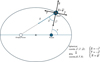Fig. A.1 Relation between spherical and RTN coordinate systems, assuming zero obliquity.

Following Segatz et al. (1988) we assume a classical synchronous rotation frame (${\widehat{\mathbf{u}}}_{{\mathbf{r}}^{\text{'}}},{\widehat{\mathbf{u}}}_{{\varphi }^{\text{'}}},{\widehat{\mathbf{u}}}_{{\lambda }^{\text{'}}}$), with zero obliquity, spin-orbit resonance, and zero forced libration. Under these assumptions, we obtain the self-figure acceleration on the body due to its degree-2 gravity: $$\mathbf{f}=\frac{{\mu }_p}{R^2}{\left(\frac{R}{a}\right)}^4{\left(\frac{r^{\text{'}}}{a}\right)}^{-4}\left(\begin{array}{c}-\frac{3}{2}{C}_{2,0}+9C_{2,2}cos\left(2{\lambda }^{\text{'}}\right)+9S_{2,2}sin\left(2{\lambda }^{\text{'}}\right)\\ 6C_{2,2}sin\left(2{\lambda }^{\text{'}}\right)-6S_{2,2}cos\left(2{\lambda }^{\text{'}}\right)\\ 0\end{array}\right)\left(\begin{array}{c}{\widehat{u}}_{r^{\text{'}}}\\ {\widehat{u}}_{{\lambda }^{\text{'}}}\\ {\widehat{u}}_{{\varphi }^{\text{'}}}\end{array}\right)$$(A.29) where, to the second order in eccentricity e (Murray & Dermott 1999): $${\left(\frac{r^{\text{'}}}{a}\right)}^{-4}\approx 1+4ecos\left(M\right)+e^2(3+7cos\left(2M\right))$$(A.30) $$sin\left(2{\lambda }^{\text{'}}\right)\approx 4esin\left(M\right)+2e^{2}sin\left(2M\right)$$(A.31) $$cos\left(2{\lambda }^{\text{'}}\right)\approx 1+e^2(4cos\left(2M\right)-4)$$(A.32) where M is the mean anomaly and a is the semimajor axis. Then, the relations in Figure A.1 are applied to obtain the RTN frame. In particular, because of the assumption of zero obliquity we have $\widehat{R}=-\widehat{r^{\text{'}}};\widehat{T}=-{\widehat{{\lambda }^{\text{'}}}}^{\text{'}};\widehat{N}={\widehat{\varphi }}^{\text{'}}$ (see Figure A.1), resulting in: $${\mathbf{f}}_{RTN}=-\frac{{\mu }_p}{R^2}{\left(\frac{R}{a}\right)}^4{\left(\frac{r^{\text{'}}}{a}\right)}^{-4}\left(\begin{array}{c}-\frac{3}{2}{C}_{2,0}+9C_{2,2}cos\left(2{\lambda }^{\text{'}}\right)+9S_{2,2}sin\left(2{\lambda }^{\text{'}}\right)\\ 6C_{2,2}sin\left(2{\lambda }^{\text{'}}\right)-6S_{2,2}cos\left(2{\lambda }^{\text{'}}\right)\\ 0\end{array}\right)\left(\begin{array}{c}{\widehat{u}}_R\\ {\widehat{u}}_T\\ {\widehat{u}}_N\end{array}\right)$$(A.33)

A.3 Static gravity

In this section we will evaluate the orbital effect due to the static degree-2 gravity field of a moon in classical synchronous rotation. Substituting Eqns. A.30, A.31, A.32 in Eq. A.33 results in the following R, T, N components: $$\begin{array}{rl}{f}_{S{T}_R}\approx & -\frac{\mu }{R^2}{\left(\frac{R}{a}\right)}^4[-\frac{3}{2}{C}_{2,0}(1+4e\cos M\\ & +e^2(3+7\cos 2M))\\ & +9C_{2,2}(1+4e\cos M+e^2(11\cos 2M-1))\\ & +18S_{2,2}(2e\sin M+5e^2\sin 2M)]\end{array}$$(A.34) $$\begin{array}{rl}{\mathit{f}}_{S{T}_T}\approx & -\frac{\mu }{R^2}{\left(\frac{R}{a}\right)}^4[12C_{2,2}(2e\sin M+5e^2\sin 2M)\\ & -6S_{2,2}(1+4e\cos M+e^2(11\cos 2M-1))]\end{array}$$(A.35) $${\mathit{f}}_{S{T}_N}=0$$(A.36)

Were subscript ST stands for static gravity. Substituting the above expressions into Eq. A.25 yields the instantaneous rate of change of the semimajor axis due to the degree-2 static gravity field, to the second order in eccentricity: $$\begin{array}{rl}{\left(\frac{da}{dt}\right)}_{ST}\approx & -{\left(\frac{R}{a}\right)}^2\sqrt{\frac{{\mu }_p}{a}}(e\sin M+3e^2\sin 2M)(-3C_{2,0}+66C_{2,2})\\ & -12S_{2,2}(1-\frac{5}{2}{e}^2+5e\cos M+17e^2\cos 2M)\end{array}$$(A.37) Then, taking the average as explained in Eqns. A.28 we get the secular rate of change: $${\langle \frac{da}{dt}\rangle }_{ST}=12\sqrt{\frac{{\mu }_p}{a}}{\left(\frac{R}{a}\right)}^2{S}_{2,2}(1-\frac{5}{2}{e}^2)$$(A.38) As shown in Eq. 43 in Section 3.2.1. Note that, importantly, under the assumption of classical synchronous rotation, S_2,2 is the only degree-2 coefficient affecting the semimajor axis, and thus the orbital energy (to the second order in eccentricity).

Analogously, substituting Eqns. A.34, A.35, and A.36 into Eq. A.26 yields the instantaneous rate of change of the orbital eccentricity: $$\begin{array}{rl}{\left(\frac{de}{dt}\right)}_{ST}\approx & -{\left(\frac{R}{a}\right)}^2\sqrt{\frac{{\mu }_p}{a^3}}[-\frac{3}{2}{C}_{2,0}(\sin M+3e\sin 2M\\ & +e^2(\frac{1}{8}\sin M+\frac{53}{8}\sin 3M))\\ & +9C_{2,2}(\sin M+\frac{17}{3}e\sin 2M\\ & +e^2(-\frac{125}{24}\sin M+\frac{415}{24}\sin 3M)\left)\right]\\ & -12S_{2,2}[\cos M+e(-\frac{1}{4}+\frac{17}{4}\cos 2M)\\ & +e^2(-\frac{7}{2}\cos M+13\cos 3M)]\end{array}$$(A.39) And averaging we get the secular variation: $${\langle \frac{de}{dt}\rangle }_{ST}\approx -3\sqrt{\frac{{\mu }_p}{a^3}}{\left(\frac{R}{a}\right)}^2{S}_{2,2}e$$(A.40) Again, only the coefficient S_2,2 influences the secular rate of change of eccentricity, under the assumption of classical synchronous rotation.

References

- Baland, R. M., Yseboodt, M., & Van Hoolst, T., 2012, Icarus, 220, 435 [NASA ADS] [CrossRef] [Google Scholar]
- Battin, R. H., 1999, An Introduction to the Mathematics and Methods of Astrodynamics (AIAA, Reston) [Google Scholar]
- Bertotti, B., Farinella, P., & Vokrouhlicky, D., 2012, Physics of the Solar System: Dynamics and Evolution, Space Physics, and Spacetime Structure (Berlin: Springer) [Google Scholar]
- Bills, B. G., Asmar, S. W., Konopliv, A. S., et al. 2014, Icarus, 240, 161 [NASA ADS] [CrossRef] [Google Scholar]
- Bolton, S. J., Lunine, J., Stevenson, D., et al. 2017, Space Sci. Rev., 213, 5 [CrossRef] [Google Scholar]
- Boué, G., & Efroimsky, M., 2019, Celest. Mech. Dyn. Astr., 131, 1 [Google Scholar]
- Cappuccio, P., Hickey, A., Durante, D., et al. 2020, Planet. Space Sci., 187, 104902 [NASA ADS] [CrossRef] [Google Scholar]
- Downey, B. G., & Nimmo, F., 2025, Sci. Adv., 11, eadl4741 [Google Scholar]
- Durante, D., Hemingway, D., Racioppa, P., et al. 2019, Icarus, 326, 123 [NASA ADS] [CrossRef] [Google Scholar]
- Eanes, R., Schutz, J., & Tapley, B., 1983, in Proc. Ninth Int. Symp. on Earth Tides, eds. J. T. Kuo (Stuttgart: Schweizerbartsche Verlagsbuchhandlung) [Google Scholar]
- Efroimsky, M., 2018, Icarus, 306, 328 [Google Scholar]
- Efroimsky, M., & Lainey, V., 2007, J. Geophys. Res., 112, E12 [Google Scholar]
- Efroimsky, M., & Makarov, V. V., 2013, ApJ, 764, 26 [NASA ADS] [CrossRef] [Google Scholar]
- Efroimsky, M., & Makarov, V. V., 2014, ApJ, 795, 6 [NASA ADS] [CrossRef] [Google Scholar]
- Efroimsky, M., & Williams, J. G., 2009, Celest. Mech. Dyn. Astr., 104, 257 [Google Scholar]
- Emelyanov, N. V., 2018, MNRAS, 479, 1278 [Google Scholar]
- Evans, S., et al. 2018, CEAS Space J., 10, 79 [NASA ADS] [CrossRef] [Google Scholar]
- Ferraz-Mello, S., Rodríguez, A., & Hussmann, H., 2008, Celest. Mech. Dyn. Astr., 101, 171 [Google Scholar]
- Folkner, W. M., Williams, J. G., Boggs, D. H., Park, R. S., & Kuchynka, P., 2014, IPN Prog. Rep., 196, 42 [Google Scholar]
- Gauss, C. F., 1906, in Carl Friedrich Gauss Werke, 7 (Göttingen: Königliche Gesellschaft der Wissenschaften), 389 [Google Scholar]
- Gomez Casajus, L., Zannoni, M., Modenini, D., et al. 2021, Icarus, 358, 114187 [NASA ADS] [CrossRef] [Google Scholar]
- Greenberg, R., & Weidenschilling, S. J., 1984, Icarus, 58, 186 [Google Scholar]
- Hay, H. C. F. C., Matsuyama, I., & Pappalardo, R. T., 2022, J. Geophys. Res., 127, e07064 [Google Scholar]
- Hemingway, D. J., & Nimmo, F., 2024, Geophys. Res. Lett., 51, e110409 [Google Scholar]
- Jacobson, R. A., 2022, AJ, 164, 199 [NASA ADS] [CrossRef] [Google Scholar]
- Kaula, W. M., 1964, Rev. Geophys., 2, 661 [Google Scholar]
- Konopliv, A. S., Park, R. S., Yuan, D. N., et al. 2013, J. Geophys. Res., 118, 1415 [Google Scholar]
- Lainey, V., Arlot, J.-E., Karatekin, O., & Van Hoolst, T., 2009, Nature, 459, 957 [NASA ADS] [CrossRef] [Google Scholar]
- Lainey, V., Karatekin, O., Desmars, J., et al. 2012, ApJ, 752, 14 [Google Scholar]
- Lainey, V., Noyelles, B., Cooper, N., et al. 2019, Icarus, 326, 48 [Google Scholar]
- Lainey, V., Casajus, L. G., Fuller, J., et al. 2020, Nat. Astron., 4, 1053 [Google Scholar]
- Magnanini, A., Zannoni, M., Casajus, L. G., et al. 2024, A&A, 687, A132 [NASA ADS] [CrossRef] [EDP Sciences] [Google Scholar]
- Mazarico, E., Genova, A., Park, R. S., et al. 2023, Space Sci. Rev., 219, 30 [NASA ADS] [CrossRef] [Google Scholar]
- Mignard, F., 1979, Moon Planets, 20, 301 [Google Scholar]
- Murray, C. D., & Dermott, S. F., 1999, Solar System Dynamics (Cambridge: Cambridge University Press) [Google Scholar]
- Noyelles, B., 2017, Icarus, 282, 276 [Google Scholar]
- Park, R. S., Folkner, W. M., Williams, J. G., & Boggs, D. H., 2021, AJ, 161, 105 [NASA ADS] [CrossRef] [Google Scholar]
- Park, R. S., Mastrodemos, N., Jacobson, R. A., et al. 2024, J. Geophys. Res., 129, e08054 [Google Scholar]
- Park, R. S., Jacobson, R. A., Gomez Casajus, L., et al. 2025, Nature, 638, 69 [Google Scholar]
- Petit, G., & Luzum, B., 2010, IERS Conventions (2010), IERS Technical Note 36 [Google Scholar]
- Rambaux, N., Van Hoolst, T., & Karatekin, O., 2011, A&A, 527, A118 [NASA ADS] [CrossRef] [EDP Sciences] [Google Scholar]
- Schubert, G., Anderson, J. D., Spohn, T., & McKinnon, W. B., 2004, in Jupiter: The Planet, Satellites and Magnetosphere, eds. F. Bagenal, T. E. Dowling, & W. B. McKinnon (Cambridge: Cambridge University Press), 281 [Google Scholar]
- Segatz, M., Spohn, T., Ross, M. N., & Schubert, G., 1988, Icarus, 75, 187 [NASA ADS] [CrossRef] [Google Scholar]
- Tobie, G., Mocquet, A., & Sotin, C., 2005, Icarus, 177, 534 [Google Scholar]
- Tortora, P., Zannoni, M., Hemingway, D., et al. 2016, Icarus, 264, 264 [NASA ADS] [CrossRef] [Google Scholar]
- Van Hoolst, T., Baland, R.-M., Trinh, A., Yseboodt, M., & Nimmo, F., 2020, J. Geophys. Res., 125, e06473 [Google Scholar]
- Williams, J. G., & Boggs, D. H., 2015, J. Geophys. Res., 120, 689 [Google Scholar]
- Williams, J. G., Boggs, D. H., Yoder, C. F., Ratcliff, J. T., & Dickey, J. O., 2001, J. Geophys. Res., 106, 27933 [Google Scholar]
- Yoder, C. F., & Peale, S. J., 1981, Icarus, 47, 1 [CrossRef] [Google Scholar]
- Zannoni, M., Hemingway, D., Casajus, L. G., & Tortora, P., 2020, Icarus, 345, 113713 [NASA ADS] [CrossRef] [Google Scholar]
It is important to note the positive sign in Eq. (26), which contrasts with the negative sign required for tides raised on a central planet by the orbiting satellite, in the typical case in which the planet spins faster than the satellite’s mean motion (Lainey et al. 2020).