© The Authors 2026

1 Introduction

The launch of the Hubble Space Telescope (HST) in 1990 revolutionized astronomy, and several space missions devoted to different scientific objectives regarding exoplanets have followed the path of HST. Among these are CoRoT (Auvergne et al. 2009), Kepler (Borucki et al. 2007; Borucki et al. 2010), and TESS (Ricker et al. 2015). So far, these missions have enabled the discovery of almost 6000 exoplanets (as well as 7000 candidates)¹. In late 2026 the PLAnetary Transits and Oscillations of stars (PLATO) mission (Rauer et al. 2014; Rauer & Heras 2018; Rauer et al. 2025) will lead to major progress in this domain. With PLATO, the number of detections of Earth-like planets will increase. Furthermore, the characterization of this type of planet in terms of radius, mass, and age will also be improved (see Heller et al. 2022).

In order to achieve its objectives, PLATO will use several stellar samples (see Montalto et al. 2021a). Sample 1 (P1) is the backbone sample of the mission, and it contains stars bright enough – i.e., lower than V=11, where the dominant noise source is the photon noise and with a maximum random noise, or random noise-to-signal ratio (NSR), of 50 ppm in one hour – to allow ground-based radial velocity (RV) follow up and detailed characterization of the host stars thanks to asteroseismology. Sample 2 (P2) consists of stars brighter than V = 8.5 with the same spectral types and noise performance as the P1 stars. Sample 4 (P4) consists of nearby cool late-type dwarf stars with habitable zones relatively close-in, meaning the planets in their habitable zone have orbital periods of only a few weeks. Sample 5 (P5), which is the largest of the four samples, is derived from the requirement of observing a large number of stars to obtain statistical information on planetary properties. Hence, with this sample more than 4000 planets are expected to be detected (see Rauer et al. 2025). However, only a small fraction of these stars can be characterized with asteroseismology (see Goupil et al. 2024) and have the mass of their planet determined with RV observations. PLATO has chosen to extract onboard photometric measurements of a large number of stars. For the brightest targets, imagettes (square regions a few pixels side of a charge-coupled device (CCD), i.e., postage-stamps in Kepler jargon) will be downloaded unprocessed to ground-based facilites. However, for most of the targets, aperture photometry will be computed on board (similarly to CoRoT, see Marchiori et al. 2019).

The PLATO mission will generate over 100 Terabits of raw data daily, far exceeding the available bandwidth for data download (see Rauer et al. 2025), namely, 435 Gbits/day. This huge data volume creates significant constraints on PLATO’s onboard CPU and telemetry systems (for more details about the onboard data processing for PLATO, we refer to the work by Ziemke et al. 2023). As a result, the mission’s onboard software must prioritize essential analyses and computations. Given these constraints, the mission strategy will rely on collecting and processing data on board for posterior ground-based validation in order to distinguish transit signals that are unlikely to be false positives (FPs). By “validation” we mean assessing a transit signal against one or several criteria to see how likely it is for the signal to be planetary (e.g., Torres et al. 2011; Díaz et al. 2014). For instance, a common procedure is to match the observed light curve to a planetary model rather than an eclipsing binary (EB) (see Lissauer et al. 2012). The word “validation” should not be confused within this context with the word “confirmation”. The confirmation of a transit signal as planetary is typically achieved by measuring the mass of the planet creating the signal, usually via RV measurements. Validation is particularly crucial for PLATO, given that confirmation through RV observations is not possible given the huge number of target stars for the mission. For instance, there will be up to ~245 000 P5 targets. Furthermore, only 4500 of the brightest P5 targets will have their photometry extracted on ground from imagettes. All of these considerations show that PLATO faces considerable constraints regarding onboard processing and telemetry due to the vast volume of generated data. Furthermore, even if it would be useful to know, it is not in the scope of this paper to realistically determine the expected EB populations for PLATO.

A well-known method for detecting as many FPs as possible and therefore making it possible to validate transit signals is measuring centroid shifts. Centroid shifts are widely used to detect FPs in ground-based transit surveys (see Günther et al. 2017) as well as in space-based transit surveys (see Batalha et al. 2010 and Bryson et al. 2013 for Kepler and Hedges 2021 for TESS)². For PLATO, centroid shift measurements were part of the initial FP detection strategy. Thus, obtaining centroids on board for at least 5% of the targets has been proposed (ESA 2021). Due to technical limitations, no more than 20% of the targets can have centroids measured on board. Furthermore, since the photometry is extracted on board for most of the targets, only the information of a very small fraction of targets is going to be downloaded to detect FPs on the ground with a series of techniques. Due to all of these reasons, the concept of double-aperture photometry was proposed since a strategy was needed for the targets that would not have centroid shift measurements.

The current strategy to detect FPs for PLATO involves a range of techniques. Two of them are the computation of centroid shifts and the use of the double-aperture photometry method. However, the efficiency of the double-aperture photometry strategy has never been assessed until now. The purpose of this paper is to provide the first overall efficiency study regarding double-aperture photometry for PLATO and its use alongside Centroid shifts, even if centroid shifts will be analyzed afterward (on ground). The idea of double-aperture photometry is to have two masks or apertures per each CCD window focused on a given star. One of these masks is the nominal mask, which is centered on the target, and it is used to extract the target photometry with the highest possible signal-to-noise ratio (S/N). The purpose of the additional mask is to measure an additional flux that, as will be shown here, enables detection of FPs under certain conditions.

We considered two options for the additional mask. One option is the “extended mask”, and the other is the “secondary mask”. The extended mask is an extension (or an expansion) of the nominal mask, making the nominal mask larger, in order to reach contaminant stars surrounding each target. The secondary mask is a smaller mask that is centered only on the most prominent contaminant around each target. With the extended mask we can obtain what we refer as to the extended flux (or extended photometry), and with the secondary mask we obtain the secondary flux (or secondary photometry). We can also use extended and secondary masks to compute centroid measurements. These centroids are alternatives to the centroids measured with the nominal mask. Similar approaches have appeared in the literature, for example, in Cabrera et al. (2017), who applied comparable vetting techniques using K2 data. However, in the context of PLATO, double-aperture photometry is advantageous, as it requires 50% less CPU and telemetry than centroid shifts³, making it an attractive alternative for onboard implementation. The approach followed in the present work can be applied to future exoplanet missions based on transit detection. This approach allows FPs to be discarded in order to enhance the selection of true positives. By “true positives” we mean transit signals coming from real planets around target stars.

The paper is organized as follows. First, we give a small overview of the PLATO mission and photometry extraction methods in Section 2. We present the proposed method of double-aperture photometry for detecting FPs and how to use it to perform flux measurements in Section 3. The centroid method for detecting FPs is described in Sect. 4. Our analysis with all the corresponding assumptions is presented in Sect. 5, and we show how we computed the efficiency of each method in Section 6. We show our results in Sect. 7 and our conclusions in Section 8.

2 PLATO mission

2.1 PLATO instrument

PLATO payload is composed of 26 cameras mounted on a single optical bench. Each camera is a 12 cm pupil diameter, wide-field refractive telescope that see ~1037 deg² (see Pertenais et al. 2021a,b). Out of the 26 cameras, 24 work at a cadence of 25 s and are called normal cameras (N-CAM). N-CAMs are used for the core science observations and are divided in four groups of six. The remaining two cameras work at a cadence of 2.5 s and are called fast cameras (F-CAM). There are four CCDs mounted on the focal plane of each N-CAM and F-CAM. Also, all N-CAMs of a given group share the same line of sight and field of view (FoV). Every ~91 days (this period of time is known as a “quarter”), the spacecraft has to rotate 90 degrees to have its solar panels directed toward the sun (see Rauer & Heras 2018).

The expected duration of the PLATO mission is four years, envisaged as two long observation phases of two years each or even one long observation of three years. If an extended mission is approved, a step-and-stare phase could be scheduled afterward. As mentioned by Nascimbeni et al. (2022), the center of both PLATO long observation phase fields are inside the spherical caps of ecliptic coordinate |β| > 63°, and the size of each field is ~2232 square degrees.

In order to fulfill the mission science objectives, four stellar samples have been defined, as mentioned in Sect. 1. For this work we only consider the P5 sample, which is often called the “statistical sample” since it will be used for planet frequency studies. This is also the sample studied by Marchiori et al. (2019) and Bray et al. (2023). The P5 sample contains at least 245 000 dwarf and sub-giant stars (F5-K7) with V ≤ 13 mag and temperatures ranging from 3875 K to 6775 K (Bray et al. 2023). The number of targets of this sample assumes two long duration observation phases.

Fig. 1 Schematic view (from left to right) of example nominal, extended, and secondary masks. For the extended and secondary masks, the respective nominal mask is represented with dashed lines. In this case, the nominal mask consists of 5 pixels, the extended mask has 19 pixels, and the secondary mask has 3 pixels. The red circle represents the target star, and the cyan triangle represents a nearby contaminant star that could be an EB. Nominal masks are used to extract target photometry and were built to have the lowest NSR. The extended masks are constructed by enlarging the nominal masks, typically by surrounding each nominal mask with a ring of one pixel. Secondary masks are typically smaller and are centered on the most problematic contaminant star in the window.

2.2 PLATO photometry

All PLATO photometric measurements, either done on board or on ground, rely on the concept of imagette. An imagette is a CCD window that surrounds a target star. The center of the imagette is located at no more than 0.5 pixels from the star barycenter (Marchiori 2019). In the case of the P5 sample the imagettes will be 6 × 6 CCD pixel squares. In particular, for the brightest targets the imagettes will be downloaded to extract their photometry on-ground. In this work we focus on the remaining P5 targets where the photometry will be extracted on board, which are the vast majority of P5 targets and that is about 80 000 stars per camera. For each one of these targets a stellar light curve will be produced on board the satellite at a cadence of 600 s or 50 s using an aperture mask. It is important to mention that there is a formal distinction between the words window and imagette for PLATO pipeline. Briefly, the word imagette refers to the 6 by 6 pixel squares that are downloaded in order to extract their photometry and centroids on-ground using a PSF fitting method. While the word window refers to the 6 by 6 squares where we compute the flux and centroid on board using an aperture.

2.3 Nominal onboard photometry

Onboard photometry extraction is done by integrating the flux over a subset of the window pixels called the aperture or the mask. Marchiori et al. (2019), in Sect. 4.6.3, showed that binary masks are the best option for PLATO and gave a procedure for obtaining a binary mask for every target. The binary mask obtained following this procedure is called the nominal mask. Furthermore, any time we refer to onboard photometry, we imply onboard photometry for N-CAM.

The main concept behind the Marchiori et al. (2019) procedure is the noise-to-signal ratio, NSR (the inverse of the S/N), of individual window pixels. The procedure of Marchiori et al. (2019) is summarized in Appendix B. Fig. 1a shows a schematic view of an example nominal mask, ω_n, obtained following this procedure. The NSR for a single PLATO pixel is $$\mathrm{N}\mathrm{S}\mathrm{R}=\frac{\text{\hspace{0.17em}Noise\hspace{0.17em}Signal\hspace{0.17em}}}{},$$(1)

where by “Signal” we mean the flux of the target and by “Noise” we mean the overall noise in a given window. For PLATO light curves computed using a binary mask, ω, and in our case a single camera, the NSR (or sometimes called N/S_*) is $${\mathrm{N}\mathrm{S}\mathrm{R}}_{\ast }=\frac{\sqrt{\sum _{\mathrm{n}=1}^{36}({\mathrm{I}}_{\mathrm{n}}^{\mathrm{T}}+\sum _{\mathrm{k}=1}^{{\mathrm{N}}_{\mathrm{C}}}{\mathrm{I}}_{\mathrm{n}}^{\mathrm{k}}+\mathrm{B}\mathrm{\Delta }{\mathrm{t}}_{\exp }+{\sigma }_{\mathrm{D}}^2+{\sigma }_{\mathrm{Q}}^2){\omega }_n}}{\sum _{\mathrm{n}=1}^{36}{\mathrm{I}}_{\mathrm{n}}^{\mathrm{T}}{\omega }_{\mathrm{n}}},$$(2)

where the subscript k runs over the number of contaminants of the imagette, N_c, the subscript n refers to the imagette pixels {1, 2, ..., 36} and ω_n refers to the binary mask over those pixels. Eq. (2) gives the NSR value for each flux measurement involving an imagette based on the noise and signal contribution of each pixel. The most recent study about the noise budget for PLATO can be found in Börner et al. (2024). Table 1 gives a complete description of the parameters in Eq. (2). For the noise related to the background flux (zodiacal light), we are using the median value from the distribution of background noise levels present in Fig. 8 of Marchiori et al. (2019). We made this choice after using the lowest (25e⁻/px/s) and highest (65e⁻/px/s) values of the distribution and realizing only a small change in our results after using both values.

For a one-hour duration signal and a given number of PLATO cameras, N_T, we can use the following expression for the NSR in ppm. hr^1/2 (assuming NSR scales with multiple independent measurements) $${\mathrm{N}\mathrm{S}\mathrm{R}}_{1\mathrm{h}}=\frac{{10}^6}{12\sqrt{{\mathrm{N}}_{\mathrm{T}}}}{\mathrm{N}\mathrm{S}\mathrm{R}}_{\ast },$$(3)

where the 12 constant refers to the square root of the number of samples in one hour for a given PLATO N-CAM, i.e., using the 25 s cadence ($\sqrt{3600s/25s}=12$).

Here, we briefly introduce the concept of PLATO data products, which represent the final outputs of the PLATO mission. The data products are organized into four levels (0–3). Level 0 includes imagettes, raw light curves, and raw centroids computed on board, while Level 1 contains processed versions of these. Level 2 involves asteroseismic parameter measurements as well as the transit planetary candidates. Finally, Level 3 data products consist of the “final catalog” of confirmed planetary systems. For this paper, we assumed that the L1 pipeline has perfectly removed the systematics and background flux of each imagette. In particular, we assumed there is no residual drift of the stars across the CCD. By “residual drift” we mean the remaining positional drift after the L1 correction. While drift and correction effectiveness do vary across the FoV, detailed assessment of this variation is part of ongoing work within the consortium.

2.4 Detectability of transit signals

In every imagette several stars surrounding the target will be present. Following the Marchiori et al. (2019) recommendation we refer as to “contaminant” any foreground star located within a 10 pixel radius from the target. Marchiori et al. (2019) showed that above a distance of 10 pixels the probability for a contaminant to generate FP is very low. Contaminants that are EBs might produce signals that can be misinterpreted as planetary transits on the target. These events are the most common examples of FPs for PLATO. In order to know the flux contribution of each contaminant to the total flux of the window, Marchiori et al. (2019) introduced the stellar-pollution ratio (SPR): $${\mathrm{S}\mathrm{P}\mathrm{R}}_{\mathrm{k}}=\frac{{\mathrm{F}}_{\mathrm{k}}}{{\mathrm{F}}_{\mathrm{t}\mathrm{o}\mathrm{t}}},$$(4)

where F_k is the flux of a single contaminant of index k and F_tot is the total flux (from all sources) present in the window. These terms are $${\mathrm{F}}_{\mathrm{k}}=\sum _{\mathrm{n}=1}^{36}{\mathrm{I}}_{\mathrm{n}}^{\mathrm{k}}{\omega }_{\mathrm{n}},$$(5) $${\mathrm{F}}_{\mathrm{t}\mathrm{o}\mathrm{t}}=\sum _{\mathrm{n}=1}^{36}{\mathrm{I}}_{\mathrm{n}}{\omega }_{\mathrm{n}},$$(6)

where ω_n is the nominal mask and where I_n is the sum of the target contribution and the contribution of all contaminant stars: $${\mathrm{I}}_{\mathrm{n}}={\mathrm{I}}_{\mathrm{n}}^{\mathrm{T}}+\sum _{\mathrm{k}=1}^{{\mathrm{N}}_{\mathrm{C}}}{\mathrm{I}}_{\mathrm{n}}^{\mathrm{k}}.$$(7)

We assumed that the sky background has been removed. However, the noise from the background flux removal remains in the expression for the NSR in Eq. (2). The total amount of pollution (i.e., total flux contribution from contaminants) in a given window is the sum of all the individual SPR_k. This metric is named the total SPR (SPR_tot): $${\mathrm{S}\mathrm{P}\mathrm{R}}_{\mathrm{t}\mathrm{o}\mathrm{t}}=\sum _{\mathrm{k}=1}^{{\mathrm{N}}_{\mathrm{C}}}{\mathrm{S}\mathrm{P}\mathrm{R}}_{\mathrm{k}}.$$(8)

The main feature of any transit signal is its transit depth, δ. This is the fraction of the area of the stellar disk that is covered during the transit. In the case of a planet transiting a star, the transit depth is called δ_p and can be approximated as $${\delta }_{\mathrm{p}}={\left(\frac{R_{\mathrm{p}}}{R_{\ast }}\right)}^2\text{,\hspace{0.17em}}$$(9)

where R_p is the radius of the planet and R_* is the radius of the star. Since we are interested in detecting FPs, we focus on the transit depth of individual background EBs, δ_EB, instead of focusing on δ_p. We recall that a given transit depth can also be defined in terms of flux. In the case of a transit happening on a contaminant star, k, the transit depth is $${\delta }_{\mathrm{E}\mathrm{B}}=\frac{{\mathrm{F}}_{\mathrm{k}}-{\mathrm{F}}_{\mathrm{k}}^{\mathrm{i}\mathrm{n}}}{{\mathrm{F}}_{\mathrm{k}}}=\frac{\mathrm{\Delta }{\mathrm{F}}_{\mathrm{k}}}{{\mathrm{F}}_{\mathrm{k}}},$$(10)

where F_k is the flux of the star out of transit and ${\mathrm{F}}_{\mathrm{k}}^{\mathrm{i}\mathrm{n}}$ is the flux of the star during a transit (i.e. ${\mathrm{F}}_{\mathrm{k}}^{\text{in\hspace{0.17em}}}=\sum _{\mathrm{n}=1}^{36}{\mathrm{I}}_{\mathrm{n}}^{\mathrm{k},\text{in}}$). The flux out of transit in the window is given by Eq. (6) and can be re-expressed as $${\mathrm{F}}^{\mathrm{o}\mathrm{u}\mathrm{t}}={\mathrm{F}}_{\mathrm{t}\mathrm{o}\mathrm{t}}={\mathrm{F}}_{\mathrm{T}}+\sum _{\mathrm{k}=1}^{{\mathrm{N}}_{\mathrm{C}}}{\mathrm{F}}_{\mathrm{k}}.$$(11)

The flux in the window when a transit is happening in a contaminant of index k is $${\mathrm{F}}^{\mathrm{i}\mathrm{n}}={\mathrm{F}}_{\mathrm{t}\mathrm{o}\mathrm{t}}+{\mathrm{F}}_{\mathrm{k}}^{\mathrm{i}\mathrm{n}}-{\mathrm{F}}_{\mathrm{k}}.$$(12)

The difference between Eq. (11) and Eq. (12) is called ΔF^nom where the superscript “nom” refers to the nominal mask and is $$\mathrm{\Delta }{\mathrm{F}}^{\mathrm{n}\mathrm{o}\mathrm{m}}={\delta }_{\mathrm{E}\mathrm{B}}{\mathrm{F}}_{\mathrm{k}},$$(13)

where δ_EB (Eq. (10)) is the intrinsic transit depth (in all the following we assume δ_EB to be given in ppm). The quantity δ_EB is also diluted by a given amount due to the flux of the target and other contaminants in the window. This causes that we are not able to measure δ_EB directly, but what we call the “observed” (or “apparent”) transit depth. This quantity is denoted as ${\delta }_{\mathrm{k}}^{\text{nom}}$ and is obtained by dividing Eq. (13) over Eq. (11) $${\delta }_{\mathrm{k}}^{\text{nom\hspace{0.17em}}}={\delta }_{\mathrm{E}\mathrm{B}}{\mathrm{S}\mathrm{P}\mathrm{R}}_{\mathrm{k}}.$$(14)

With this we were able to define the statistical significance of the transit. First we recall that the statistical significance, η, of the transit is the ratio of the apparent transit depth, ${\delta }_{\mathrm{k}}^{\text{nom}}$, over the noise. The expression for the statistical significance in the nominal mask for a transit happening in a contaminant star is $${\eta }_{\mathrm{k}}^{\mathrm{n}\mathrm{o}\mathrm{m}}=\frac{{\delta }_{\mathrm{k}}^{\mathrm{n}\mathrm{o}\mathrm{m}}{\mathrm{F}}_{\mathrm{t}\mathrm{o}\mathrm{t}}\sqrt{{\mathrm{t}}_{\mathrm{E}\mathrm{B}}{\mathrm{n}}_{\mathrm{t}\mathrm{r}}}}{{\sigma }_{{\mathrm{F}}_{\mathrm{t}\mathrm{o}\mathrm{t}}}},$$(15)

where t_EB and n_tr are, respectively, the transit duration (in hours) and number of transits, and σ_Ftot is the 1-σ dispersion in the light-curve averaged over 1 hour and over N_T cameras. We do this 1-hour average because we are using transit durations expressed in hours and also because measurements have to be averaged over the duration of a transit, that typically last only a few hours. By definition we have (see Eq. (1)) $${\mathrm{N}\mathrm{S}\mathrm{R}}_{1\mathrm{h}\mathrm{r}}\equiv \frac{{\sigma }_{{\mathrm{F}}_{\mathrm{t}\mathrm{o}\mathrm{t}}}}{{\mathrm{F}}_{\mathrm{T}}}.$$(16)

Furthermore, $$\frac{{\mathrm{F}}_{\mathrm{T}}}{{\mathrm{F}}_{\mathrm{t}\mathrm{o}\mathrm{t}}}=1-{\mathrm{S}\mathrm{P}\mathrm{R}}_{\mathrm{t}\mathrm{o}\mathrm{t}}.$$(17)

Accordingly, with the help of Eqs. (14), (16) and (17), Eq. (15) can be rewritten as $${\eta }_{\mathrm{k}}^{\mathrm{n}\mathrm{o}\mathrm{m}}=\frac{{\delta }_{\mathrm{E}\mathrm{B}}{\mathrm{S}\mathrm{P}\mathrm{R}}_{\mathrm{k}}\sqrt{{\mathrm{t}}_{\mathrm{E}\mathrm{B}}{\mathrm{n}}_{\mathrm{t}\mathrm{r}}}}{(1-{\mathrm{S}\mathrm{P}\mathrm{R}}_{\mathrm{t}\mathrm{o}\mathrm{t}}){\mathrm{N}\mathrm{S}\mathrm{R}}_{1\mathrm{h}}},$$(18)

where NSR_1h is given by Eq. (3). As can be seen, the significance scales with ${\delta }_{\mathrm{E}\mathrm{B}}\sqrt{{\mathrm{t}}_{\mathrm{E}\mathrm{B}}}$, whose value varies depending on the star.

In order to be detectable, any transit signal should have a statistical significance value above a given threshold. We call this threshold η_min. Based on considerations given by Jenkins et al. (2010), Marchiori et al. (2019) used η_min = 7.1 for their analysis. More recent studies (e.g., Hsu et al. 2018; Christiansen et al. 2020; Kunimoto & Matthews 2020; Bryson et al. 2020) have challenged this choice. However, we keep it for consistency with the study by Marchiori et al. (2019). It follows that a contaminant star that is an EB generates a significant transit in the nominal flux (FP) whenever we have $${\eta }_{\mathrm{k}}^{\text{nom}}>{\eta }_{min}.$$(19)

Following Marchiori et al. (2019), it is possible to derive a threshold in terms of SPR above which a transit in a contaminant star can cause an FP. Indeed, using Eqs. (18) and (19), it can be shown that this happens when $${\mathrm{S}\mathrm{P}\mathrm{R}}_{\mathrm{k}}>{\mathrm{S}\mathrm{P}\mathrm{R}}_{\mathrm{k}}^{\text{crit\hspace{0.17em}}},$$(20)

where $${\mathrm{S}\mathrm{P}\mathrm{R}}_{\mathrm{k}}^{\mathrm{c}\mathrm{r}\mathrm{i}\mathrm{t}}=\frac{{\eta }_{min}(1-{\mathrm{S}\mathrm{P}\mathrm{R}}_{\mathrm{t}\mathrm{o}\mathrm{t}}){\mathrm{N}\mathrm{S}\mathrm{R}}_{1\mathrm{h}}}{{\delta }_{\mathrm{E}\mathrm{B}}\sqrt{{\mathrm{t}}_{\mathrm{E}\mathrm{B}}{\mathrm{n}}_{\mathrm{t}\mathrm{r}}}},$$(21)

is by definition the critical SPR.

For completeness, we write the statistical significance in the nominal mask of a planet transiting the target star: $$\eta =\frac{{\delta }_{\mathrm{p}}\sqrt{{\mathrm{t}}_{\mathrm{p}}{\mathrm{n}}_{\mathrm{t}\mathrm{r}}}}{{\mathrm{N}\mathrm{S}\mathrm{R}}_{1\mathrm{h}}},$$(22)

where δ_p, t_p and n_tr are, respectively, the planet transit depth (in ppm), the transit duration in hours and the observed number of transits (metrics such as Eq. (22) are called MES: Multiple Event Statistic in Kepler jargon).

We remark that Eqs. (21) and (22) are, respectively, corrected versions of Eqs. (28) and (23) in Marchiori et al. (2019). The corrections address the proper placement of the (1 – SPR_tot) factor to ensure mathematically consistent flux ratio treatments between target and total flux measurements. In more detail, the proper treatment of target flux (F_T) to total flux (F_tot) ratios requires F_T/F_tot = 1 – SPR_tot, which was incorrectly applied in the original formulations.

3 Double-aperture photometry and flux measurements for detecting FPs

The idea of the double-aperture photometry is to use an extra aperture to compute an alternative photometry to the nominal photometry in order to detect FPs. Here we consider two versions of double-aperture photometry: the extended mask and the secondary mask. Sections 3.1 and 3.2 respectively present and describe each one of these masks. Sect. 6 explains that extended and secondary masks can also be used alongside centroid shift measurements. This allows the extended centroids to be created when using extended masks as well as the secondary centroids when using secondary masks. In Sect. 8, we draw a scheme to indicate different applicable scenarios for each mask.

3.1 Extended mask and extended flux

The extended mask is an expansion of the nominal mask. Given the scenario of a target surrounded by contaminants, collecting their flux is useful to look for FPs. In order to collect that contaminant flux we increase the size of the nominal mask. This is done to reach as much contaminants as possible. The expansion process is done by surrounding the nominal mask by a given number of pixels, typically one pixel, in order to avoid increasing the noise significantly. Fig. 1b shows an schematic representation of how an extended mask is built.

At window level, there will be an overlap between the nominal and the extended masks. A large fraction of the flux collected by the extended mask comes from the target. However, the extended mask collect a larger fraction of the flux from the contaminant stars compared to the nominal mask, and hence it is more sensitive to the existence of a transit on a contaminant star. From this perspective the extended mask can be seen as a nominal mask that is more sensitive to all the contaminant flux in the imagette. If a transit happens in a contaminant star of index k, the observed transit depth in the extended mask is called ${\delta }_{\mathrm{k}}^{\text{ext}}$ and is $${\delta }_{\mathrm{k}}^{\mathrm{e}\mathrm{x}\mathrm{t}}={\delta }_{\mathrm{E}\mathrm{B}}{\mathrm{S}\mathrm{P}\mathrm{R}}_{\mathrm{k}}^{\mathrm{e}\mathrm{x}\mathrm{t}},$$(23)

where ${\mathrm{S}\mathrm{P}\mathrm{R}}_{\mathrm{k}}^{\text{ext}}$ is computed with Eq. (4) by using the extended mask. We can define the statistical significance in the extended mask for a transit happening in a contaminant star $${\eta }_{\mathrm{k}}^{\mathrm{e}\mathrm{x}\mathrm{t}}=\frac{{\delta }_{\mathrm{E}\mathrm{B}}{\mathrm{S}\mathrm{P}\mathrm{R}}_{\mathrm{k}}^{\mathrm{e}\mathrm{x}\mathrm{t}}\sqrt{{\mathrm{t}}_{\mathrm{E}\mathrm{B}}{\mathrm{n}}_{\mathrm{t}\mathrm{r}}}}{(1-{\mathrm{S}\mathrm{P}\mathrm{R}}_{\mathrm{t}\mathrm{o}\mathrm{t}}^{\mathrm{e}\mathrm{x}\mathrm{t}}){\mathrm{N}\mathrm{S}\mathrm{R}}_{1\mathrm{h}}^{\mathrm{e}\mathrm{x}\mathrm{t}}},$$(24)

where ${\mathrm{S}\mathrm{P}\mathrm{R}}_{\text{tot}}^{\text{ext}}$ and ${\mathrm{N}\mathrm{S}\mathrm{R}}_{1\mathrm{h}}^{\text{ext}}$ are, respectively, Eqs. (2) and (8) assuming an extended mask. Since the photometry extraction for each mask is performed separately, two light curves will be created per window: one based on the nominal mask and the other on the extended mask. The light curve produced with the extended mask is used to detect FPs since the extended mask might enhance any transit signal coming from the contaminants. For instance, if we have a transit signal in the nominal light curve but an even deeper transit signal in the extended light curve, we can conclude that the origin of the signal is not the target but it is due to one of the contaminant stars located nearby the target. In other words we are dealing with a FP that thanks to the extended mask we can identify as such. The physical explanation for this relies on dilution effects: if a genuine planet transits the target star, the extended light curve will exhibit equal or shallower transit depth than the nominal curve due to additional flux from nearby stars in the larger aperture. Extended transits that are deeper than nominal transits are therefore physically incompatible with target-star planets and can only arise from contaminating EBs.

Of course, by increasing the size of the mask we are also increasing the NSR (lowering the S/N) of the photometric signature of the background transit, which means that a trade-off has to be established. For instance, it would be enough to increase the size of the extended mask by one more pixel and see the impact on the efficiency. This has been done already by Gutierrez Canales (2025), where Fig. 7.1 shows that creating extended masks by extending nominal masks beyond the single-pixel ring significantly reduces flux efficiency, likely because the added pixels increase noise more than signal. Therefore, even if more optimal ways to build extended masks could be implemented (ongoing work in the mission consortium), such as adding only specific pixels to the nominal mask (see Sect. 8.4), we opted for the 1-pixel ring approach for the rest of this work for the sake of simplicity.

3.2 Secondary mask and secondary flux

The idea behind the concept of a secondary mask is to collect the flux only from one contaminant in each window. That contaminant is the one with the highest SPR_k value. This is the reason we sometimes refer to that contaminant as the most prominent. The reason behind this choice is that the contaminant with the highest SPR_k value is also the most probable to cause an FP. However, the observed transit depth of a transit happening in the most prominent contaminant star in the secondary mask, ${\delta }_{\mathrm{k}\mathrm{m}\mathrm{a}\mathrm{x}}^{\mathrm{s}\mathrm{e}\mathrm{c}}$, can be diluted by nearby contaminants. This is expressed as $${\delta }_{\mathrm{k}\mathrm{m}\mathrm{a}\mathrm{x}}^{\mathrm{s}\mathrm{e}\mathrm{c}}={\delta }_{\mathrm{E}\mathrm{B}}{\mathrm{S}\mathrm{P}\mathrm{R}}_{\mathrm{k}\mathrm{m}\mathrm{a}\mathrm{x}}^{\mathrm{s}\mathrm{e}\mathrm{c}},$$(25)

where ${\mathrm{S}\mathrm{P}\mathrm{R}}_{\mathrm{k}}^{\text{sec}}$ is computed with Eq. (4) by using the secondary mask. Then, as done for the nominal mask (see Sect. 2.4), we derived the statistical significance in the secondary mask for a transit happening in the most prominent contaminant star: $${\eta }_{\mathrm{k}\mathrm{m}\mathrm{a}\mathrm{x}}^{\mathrm{s}\mathrm{e}\mathrm{c}}=\frac{{\delta }_{\mathrm{E}\mathrm{B}}\sqrt{{\mathrm{t}}_{\mathrm{E}\mathrm{B}}{\mathrm{n}}_{\mathrm{t}\mathrm{r}}}}{{\mathrm{N}\mathrm{S}\mathrm{R}}_{1\mathrm{h}}^{\mathrm{s}\mathrm{e}\mathrm{c}}},$$(26)

where ${\mathrm{N}\mathrm{S}\mathrm{R}}_{1\mathrm{h}}^{\text{sec}}$ refers to Eq. (2) assuming a secondary mask and the most prominent contaminant in the window having the role of the target. This means that ${\mathrm{I}}_{\mathrm{n}}^{\mathrm{k}\mathrm{m}\mathrm{a}\mathrm{x}}$ appears in the denominator of ${\mathrm{N}\mathrm{S}\mathrm{R}}_{1\mathrm{h}}^{\text{sec}}$. The secondary mask can be seen as a nominal mask that is centered not in the target but in the contaminant with the highest value of SPR_k in the window. This is the reason Eq. (26) is formally equivalent to Eq. (22), which corresponds to the significance of the planet transiting the target star. From this perspective, the process to obtain the secondary mask is analogous to the one for obtaining the nominal mask (described in Appendix B). Given the fact that most contaminants are fainter than the target, the resulting secondary mask is typically only a few pixels in size. This is why secondary masks have – in most cases – a lower NSR (high S/N) than the extended masks. Fig 1c shows an example view of the secondary mask.

As for the extended mask, two light curves will be produced for every window containing a nominal and a secondary mask. This “secondary” light curve can be used to detect FPs in the following way: if we have a transit signal in the nominal mask but an even deeper transit in the secondary mask, we can conclude that the origin of the signal in the nominal mask was in fact the star where the secondary mask is centered. From this perspective, the secondary mask works as a focused nominal mask that enhances the transit signal from a single, specific contaminant, instead of dealing with several contaminants at the same time, as in the case of the extended mask. However, this can also be seen as a possible drawback for secondary masks, specially for very crowded windows. If more than one contaminant can create an FP in a window, monitoring as much contaminants as possible is crucial. In Sect. 8.1 we explore this in more detail.

4 Centroid shifts for detecting FPs

The centroid shift method is based on detecting a shift in the center of brightness of a window whenever there is a transit. When we refer to the centroid (often called the “center of brightness” or “photocenter”) of a given window, we refer to the coordinates of the geometric center of all the flux sources in the window. Centroid measurements are computed using only pixels within a given aperture. We recall that – for the targets for which photometry is extracted on board – the current strategy for PLATO to detect FPs includes the computation of centroid shifts using the nominal mask. However, just a small amount of P5 targets will have those measurements.

When no transits occur, the centroid of the window remains close to the target. If there is a transit on the target, a small centroid shift is created. If a transit happens on a contaminant star that is bright and distant enough, but not too far away, from the target, the resulting centroid is enhanced. As pointed out by Günther et al. (2017), if the system (target plus contaminants) can be visually resolved, the direction of the shift indicates which object undergoes the eclipse.

The coordinates of the centroid in the window reference frame are $${\mathrm{C}}_{\mathrm{x}}=\frac{\sum _{\mathrm{n}=1}^{36}{\mathrm{x}}_{\mathrm{n}}{\mathrm{I}}_{\mathrm{n}}{\omega }_{\mathrm{n}}}{{\mathrm{F}}_{\mathrm{t}\mathrm{o}\mathrm{t}}},{\mathrm{C}}_{\mathrm{y}}=\frac{\sum _{\mathrm{n}=1}^{36}{\mathrm{y}}_{\mathrm{n}}{\mathrm{I}}_{\mathrm{n}}{\omega }_{\mathrm{n}}}{{\mathrm{F}}_{\mathrm{t}\mathrm{o}\mathrm{t}}},$$(27)

where F_tot is given in Eq. (6), I_n is the total intensity in the pixel of order n (Eq. (7)), x_n is the row coordinate of the center of every pixel in the window frame, y_n is consequently the column coordinate of the center of every pixel in the window frame and ω_n is the considered mask.

When a background transit occurs, I_n in Eq. (27) is replaced by ${\mathrm{I}}_{\mathrm{n}}^{\mathrm{i}\mathrm{n}}$, which is the total intensity in the pixel of order n during the transit. Any centroid shift is always associated with a given contaminant, k, which we suppose is an EB. The corresponding x and y coordinates of the centroid during the transit are called, respectively, ${\mathrm{C}}_{\mathrm{x}}^{\mathrm{k},\text{in}}$ and ${\mathrm{C}}_{\mathrm{y}}^{\mathrm{k},\text{in}}$. We note that the centroid shift in the transit is indexed with k since it depends on the contaminant of index k at the origin of the background transit.

At this point, we could define the centroid shift in each direction. The change in the position of the centroid alongside the x direction is $\mathrm{\Delta }{\mathrm{C}}_{\mathrm{x}}^{\mathrm{k}}={\mathrm{C}}_{\mathrm{x}}-{\mathrm{C}}_{\mathrm{x}}^{\mathrm{k},\mathrm{i}\mathrm{n}}$, and the change alongside the y direction is $\mathrm{\Delta }{\mathrm{C}}_{\mathrm{y}}^{\mathrm{k}}={\mathrm{C}}_{\mathrm{y}}-{\mathrm{C}}_{\mathrm{y}}^{\mathrm{k},\text{in}}$. The absolute (or total) centroid shift is $$\mathrm{\Delta }{\mathrm{C}}^{\mathrm{k}}=\sqrt{{\left(\mathrm{\Delta }{\mathrm{C}}_{\mathrm{x}}^{\mathrm{k}}\right)}^2+{\left(\mathrm{\Delta }{\mathrm{C}}_{\mathrm{y}}^{\mathrm{k}}\right)}^2}.$$(28)

We also defined the centroid shift alongside one direction in terms of the transit depth as follows: $$\mathrm{\Delta }{\mathrm{C}}_{\mathrm{x}}^{\mathrm{k}}={\lambda }_{\mathrm{k}}[\delta ]{\mathrm{\Gamma }}_{\mathrm{x}}^{\mathrm{k}},$$(29)

where $${\lambda }_{\mathrm{k}}\left[{\delta }_{\mathrm{E}\mathrm{B}}\right]=\frac{{\delta }_{\mathrm{E}\mathrm{B}}\times {10}^{-6}}{1-{\delta }_{\mathrm{E}\mathrm{B}}\times {10}^{-6}{\mathrm{S}\mathrm{P}\mathrm{R}}_{\mathrm{k}}},$$(30)

and $${\mathrm{\Gamma }}_{\mathrm{x}}^{\mathrm{k}}=\frac{\sum _{\mathrm{n}=1}^{36}({\mathrm{x}}_{\mathrm{n}}-{\mathrm{C}}_{\mathrm{x}}){\omega }_{\mathrm{n}}{\mathrm{I}}_{\mathrm{n}}^{\mathrm{k}}}{{\mathrm{F}}_{\mathrm{t}\mathrm{o}\mathrm{t}}}.$$(31)

We recall that in this work the transit depths are assumed to be in parts per million. This requires conversion to dimensionless fractions (×10⁻⁶) such as the one in Eq. (30). The absolute centroid shift can therefore be rewritten as $$\mathrm{\Delta }{\mathrm{C}}_{\mathrm{k}}={\lambda }_{\mathrm{k}}\left[{\delta }_{\mathrm{E}\mathrm{B}}\right]\sqrt{{\left({\mathrm{\Gamma }}_{\mathrm{x}}^{\mathrm{k}}\right)}^2+{\left({\mathrm{\Gamma }}_{\mathrm{y}}^{\mathrm{k}}\right)}^2}={\lambda }_{\mathrm{k}}\left[{\delta }_{\mathrm{E}\mathrm{B}}\right]{\mathrm{\Gamma }}_{\mathrm{k}},$$(32)

where we have defined $${\mathrm{\Gamma }}_{\mathrm{k}}=\sqrt{{\left({\mathrm{\Gamma }}_{\mathrm{x}}^{\mathrm{k}}\right)}^2+{\left({\mathrm{\Gamma }}_{\mathrm{y}}^{\mathrm{k}}\right)}^2}.$$(33)

4.1 Centroid shift error

In order to compute the error for the absolute centroid shift, we needed to compute first the error for the shift in each direction. We introduced the term $\delta {\mathrm{I}}_{\mathrm{n}}={\mathrm{I}}_{\mathrm{n}}-{\overline{\mathrm{I}}}_{\mathrm{n}}$ as an additional help in our calculations. The term ${\overline{\mathrm{I}}}_{\mathrm{n}}$ refers to the mean of the variable I_n, which is given by Eq. (7). We could thus write the variances as $$\mathrm{Var}\left(\delta {\mathrm{I}}_{\mathrm{n}}\right)={\overline{\mathrm{I}}}_{\mathrm{n}}+\mathrm{B}\mathrm{\Delta }{\mathrm{t}}_{\mathrm{e}\mathrm{x}\mathrm{p}}+{\sigma }_{\mathrm{D}}^2+{\sigma }_{\mathrm{Q}}^2,$$(34)

where $\mathrm{B},\mathrm{\Delta }{\mathrm{t}}_{\text{exp}},{\sigma }_{\mathrm{D}}^2,{\sigma }_Q^2$ are the quantities involved in Eq. (2) and their values are given in Table 1. With this new term, we could compute the noise associated with the centroid in the x direction, ${\sigma }_{\mathrm{x}}^2$, as follows (the noise for the centroid in the y direction is analogous): $${\sigma }_{\mathrm{x}}^2=\frac{\sum _{n=1}^{36}{({\mathrm{x}}_{\mathrm{n}}-{\mathrm{C}}_{\mathrm{x}})}^2{\omega }_{\mathrm{n}}\mathrm{Var}\left(\delta {\mathrm{I}}_{\mathrm{n}}\right)}{{\mathrm{F}}_{\mathrm{t}\mathrm{o}\mathrm{t}}^2}.$$(35)

Equation (35) is actually a revision of Eq. (2) from Bryson et al. (2013), which is not invariant under translations of the reference system.

The error for the absolute centroid shift is therefore $${\sigma }_{{\mathrm{\Delta }}_C}=\frac{1}{\mathrm{\Delta }C}\sqrt{\mathrm{\Delta }{\mathrm{C}}_{\mathrm{x}}^2{\sigma }_{\mathrm{x}}^2+\mathrm{\Delta }{\mathrm{C}}_{\mathrm{y}}^2{\sigma }_{\mathrm{y}}^2},$$(36)

where we assumed a larger number of out-of-transit centroid measurements than for the in-transit ones. This gives more precision for the out-of-transit centroids than for the in-transit centroids. Accordingly, we can assume ${\sigma }_{\mathrm{x}}^{\text{out}}\ll {\sigma }_{\mathrm{x}}^{\text{in}}$ (and analogously ${\sigma }_{\mathrm{y}}^{\text{out}}\ll {\sigma }_{\mathrm{y}}^{\text{in}}$).

Furthermore, Eq. (36) is equivalent to Eq. (7) from Bryson et al. (2013). There is, however, a difference in the reference system of both papers. In this work the reference system for the centroid computations is the CCD reference frame while Bryson et al. (2013) use equatorial coordinates (RA and declination).

To derive Eq. (36), we have assumed that the centroid error is always significantly smaller than the centroid shift itself. As can be seen, Eq. (36) goes to zero as the centroid shift, ΔC, goes to zero. However, this is problematic for scenarios where the centroid shift is very small and comparable to the centroid error. One of these scenarios is the one where centroid shifts are computed with secondary masks of only one pixel in size. For such cases centroid shifts are naturally zero, and therefore Eq. (36) no longer holds. More details about how we avoided such cases are given in Sects. 6.2.1, 6.2.2, and 6.2.3.

4.2 Significance of the centroid

We can define the statistical significance of a centroid shift signal by taking into account some PLATO specifications and scientific requirements. For instance we can average centroid measurements over a duration of one hour and a given number of cameras, N_T, in order to reduce the uncertainty as follows: $${\sigma }^{1\mathrm{h},{\mathrm{N}}_{\mathrm{T}}}=\frac{{\sigma }_{{\mathrm{\Delta }}_{\mathrm{C}}}}{12\sqrt{{\mathrm{N}}_{\mathrm{T}}}}.$$(37)

We recall that in a parallel way to the flux measurements described in Sect. 2.4, we computed the centroid uncertainty after averaging the centroid over one hour.

The corresponding statistical significance of the centroid shift in the nominal mask for a transit happening in a contaminant star is $${\eta }_k^{\mathrm{n}\mathrm{o}\mathrm{m},\mathrm{\Delta }\mathrm{C}}=\frac{\mathrm{\Delta }{\mathrm{C}}_{\mathrm{k}}\sqrt{{\mathrm{t}}_{\mathrm{E}\mathrm{B}}{\mathrm{n}}_{\mathrm{t}\mathrm{r}}}}{{\sigma }^{1\mathrm{h},{\mathrm{N}}_{\mathrm{T}}}}=\frac{{\lambda }_{\mathrm{k}}\left[{\delta }_{\mathrm{E}\mathrm{B}}\right]{\mathrm{\Gamma }}_{\mathrm{k}}^{\mathrm{n}\mathrm{o}\mathrm{m}}\sqrt{{\mathrm{t}}_{\mathrm{E}\mathrm{B}}{\mathrm{n}}_{\mathrm{t}\mathrm{r}}}}{{\sigma }^{1\mathrm{h},{\mathrm{N}}_{\mathrm{T}}}}.$$(38)

While the significance of the background transit in the flux scales as ${\delta }_{\mathrm{E}\mathrm{B}}\sqrt{{\mathrm{t}}_{\mathrm{E}\mathrm{B}}}$, the statistical significance of the centroid shift rather scales as $\lambda \left[{\delta }_{\mathrm{E}\mathrm{B}}\right]\sqrt{{\mathrm{t}}_{\mathrm{E}\mathrm{B}}}$. However, the denominator in Eq. (30) is for most contaminant stars close to 1 such that in most cases λ ∝ δ_k. Accordingly, we can consider that as for the significance in terms of photometry (Eq. (18)), the significance of the centroid shift predominantly scales as ${\delta }_{\mathrm{E}\mathrm{B}}\sqrt{{\mathrm{t}}_{\mathrm{E}\mathrm{B}}}$.

The subscript “nom” in Eq. (38) indicates that we are using the nominal mask. However, we can replace the nominal mask with either the extended or secondary masks and have the following equivalent expressions: $${\eta }_k^{\mathrm{e}\mathrm{x}\mathrm{t},\mathrm{\Delta }\mathrm{C}}=\frac{{\lambda }_{\mathrm{k}}\left[{\delta }_{\mathrm{E}\mathrm{B}}\right]{\mathrm{\Gamma }}_{\mathrm{k}}^{\mathrm{e}\mathrm{x}\mathrm{t}}\sqrt{{\mathrm{t}}_{\mathrm{E}\mathrm{B}}{\mathrm{n}}_{\mathrm{t}\mathrm{r}}}}{{\sigma }_{\mathrm{e}\mathrm{x}\mathrm{t}}^{1\mathrm{h},{\mathrm{N}}_{\mathrm{T}}}}.$$(39) $${\eta }_k^{\mathrm{s}\mathrm{e}\mathrm{c},\mathrm{\Delta }\mathrm{C}}=\frac{{\lambda }_{\mathrm{k}}\left[{\delta }_{\mathrm{E}\mathrm{B}}\right]{\mathrm{\Gamma }}_{\mathrm{k}}^{\mathrm{s}\mathrm{e}\mathrm{c}}\sqrt{{\mathrm{t}}_{\mathrm{E}\mathrm{B}}{\mathrm{n}}_{\mathrm{t}\mathrm{r}}}}{{\sigma }_{\mathrm{s}\mathrm{e}\mathrm{c}}^{1\mathrm{h},{\mathrm{N}}_{\mathrm{T}}}},$$(40)

where ${\sigma }_{\text{ext}}^{1\mathrm{h},{\mathrm{N}}_{\mathrm{T}}}$ and ${\sigma }_{\text{sec}}^{1\mathrm{h},{\mathrm{N}}_{\mathrm{T}}}$ refers to Eq. (37) but using respectively the extended and secondary masks instead.

5 Methods and assumptions

In this section, we present our methodology and key assumptions, particularly those regarding contaminant stars and EBs. We recall that our goal is to see how efficient are flux and centroid shift measurements when using double-aperture photometry for detecting FPs. For this goal, we compared the flux and centroid measurements based on our alternative apertures (extended and secondary masks) with the centroid shifts computed with the nominal mask.

5.1 Stellar sample

We used a stellar sample with data from Gaia Data Release 3 (DR3) (Gaia Collaboration 2016, 2023). Our sample contains 13.6 million of stars, ranging from magnitude 2.1 up to 21 in the Gaia band. This magnitude range and cutoff for faint targets comes from Gaia DR3, rather than PLATO sensitivity constraints. The sample was selected based on an approximation of the number of stars in the FoV of a single PLATO N-CAM for a single pointing at the center of the SPF (Southern PLATO Field). However, we note that this is only somewhat representative of what the true respective PLATO sample would resemble. For simplicity, we did not take into account the proper motion of any star in the Gaia catalog. We converted the magnitude of the stars in the sample from the Gaia band to the PLATO magnitude system by using Eq. (9) from Marchiori et al. (2019), where P is related to G, G_bp, and G_rp magnitudes measured by Gaia. Afterward, and taking into account PLATO P5 sample specifications described in Sect. 2.1, we defined as a target every star with magnitude between 8.0 ≤ P ≤ 13.0. We defined as contaminant stars any star in the whole magnitude range of the sample, within a distance of 10 pixels for every target. This since the probability of having an FP generated by a contaminant located at a distance larger than 10 pixels is very low according to Marchiori et al. (2019).

5.2 Assumptions about background eclipsing binaries

In principle, the information that PLATO will have about contaminant stars comes from Gaia and the PLATO Input Catalog (PIC) (see Montalto et al. 2021b), where a flag system for EBs can be implemented. However, there are studies about EB populations such as Söderhjelm & Dischler (2005) and Mowlavi et al. (2023). This last one is of particular interest since they report approximately two million EB candidates identified with Gaia. In terms of EB occurrence rates for space missions, we can mention Prša et al. (2011) that reported and EB occurrence of 1.2% for Kepler⁴ and Prša et al. (2022) that reported an EB occurrence of 3% at low Galactic latitudes for TESS. However, even if we recognize that it is not feasible to know all contamination sources for each individual window or imagette for PLATO in advance, our aim here is not to estimate realistic EB rates for PLATO, as we mentioned in the introduction, and we refer to the work by Bray et al. (2023) on that regard. Another important assumption of this work is related to stellar variability. We did not include in our flux or centroid shift calculations intrinsic stellar variability out for simplicity.

Following Marchiori et al. (2019), we assumed that all contaminants in this work are EBs but instead of assuming that all EBs have the same transit depth and duration, we refined their approach by drawing their properties from known distributions. For each EB we randomly sampled (δ_EB, t_EB) pairs from the Kepler Eclipsing Binary Catalog (Kirk et al. 2016)⁵ and transit duration distribution in the Certified FP Table.⁶ However, we note that assuming all contaminants are EBs represents a worst-case scenario for contamination. This allowed us to assess the maximum capability of each detection method under challenging conditions.

5.3 Instrument performance and PSF assumptions

The point-spread function (PSF) describes how a stellar signal is distributed after interacting with the optics of an instrument. In the case of PLATO, the PSF determined how the stellar signal is distributed over the pixels of the detectors. We used 4224 PLATO-representative PSFs that were created in ZEMAX by simulating the baseline optical layout of the instrument. These PSFs also include miss-alignment and mounting errors. They were computed for the PLATO reference 6000 K G0V star and for the best focus (0 μm distance to the best focus).

Furthermore, a convolution with a Gaussian kernel with a given width was applied on each PSF to mimic the charge diffusion effect in PLATO CCDs. Two widths were adopted, 0.1 px and 0.2 px. The difference between the results produced with each width is marginal. At the end we adopted the PSFs convoluted with a 0.2 px width kernel. We made this decision because CCD diffusion strongly depends on the effective temperature of an observed star and a 0.2 px width approximates the aforementioned case of PLATO reference stellar source: a 6000 K GOV star.

Once we obtained the PSFs, we looked for their coordinates in the focal plane to find the closest one to each target star. After this process, we decomposed every PSF into b-spline polynomials that are analytically integrable. This is done to accurately integrate the PSF over a given array of pixels, in our case, a 6 × 6 pixel window. For this work, we assumed that each camera has the same set of PSFs. Each PSF is, however, not constant, as each PSF varies across the whole FoV. Furthermore, our PSF set reflects realistic camera-to-camera variations based on Monte Carlo simulations of alignment and mounting errors. These simulations were carried out by a member of the PLATO Mission Consortium (PMC) and distributed within the consortium. Fig. 2 shows some example PSFs used in our work. The PSFs are shown at three different angles of the FoV of one camera, before and after adding the diffusion effect. The corresponding windows for each PSF are shown in the last column of the figure. The PLATO cameras are designed to enclose about 77% of the PSF flux within a 2.5 pixel window and 99% of the flux within a 5x5 pixel window. We also notice that photometry performance depends on the knowledge of the PSF and the shape of the PSF is expected to change after launch. This implies that the “true” PSF cannot be obtained. In order to reconstruct the “true” PSF a microscanning technique will be implemented on board (see Samadi et al. 2019).

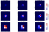Fig. 2 Simulated PLATO PSFs (1/64 pixel resolution) at different angular positions, α, of a flux source in the FoV of a PLATO camera. When α = 0° the source is in the center of the FoV and when α = 18° the source is at the edge of the FoV. The top row shows the PSFs without charge diffusion, while in the middle row a Gaussian kernel was applied to simulate charge diffusion in the CCD. The bottom row shows the PSF integrated over the pixels of a 6x6 window. The color scheme goes from the highest value (red) to the smallest values (blue).

6 Efficiency of flux and centroid shift measurements for detecting FPs

6.1 Efficiency of flux measurements

6.1.1 Efficiency of extended flux

Determining the efficiency of extended flux measurements requires two quantities. The first quantity is the total number of FPs expected for the nominal mask, which we call N_FP. It is given by the number of contaminants per window for which Eq. (19) holds (${\eta }_{\mathrm{k}}^{\mathrm{n}\mathrm{o}\mathrm{m}}>{\eta }_{min}$). This is written as $${\mathrm{N}}_{\mathrm{F}\mathrm{P}}=\sum _{\text{targets\hspace{0.17em}}}(\sum _{\mathrm{k}=1}^{{\mathrm{N}}_{\mathrm{C}}=10}{\eta }_{\mathrm{k}}^{\mathrm{n}\mathrm{o}\mathrm{m}}>{\eta }_{min}).$$(41)

We recall that η_min = 7.1. To compute N_FP we have to obtain the value of ${\eta }_{\mathrm{k}}^{\mathrm{n}\mathrm{o}\mathrm{m}}$ for every contaminant in the window and then compare it to η_min. However, the number of contaminants per window, N_c, can be up to hundreds. For simplicity, we computed ${\eta }_{\mathrm{k}}^{\text{nom}}$ for only the ten most significant contaminant stars in the window, based on their SPR_k values. Section 7 justifies this approach, as only a few contaminants per window can induce an FP.

The second quantity for computing the efficiency of the extended mask is the number of detectable FPs by the extended mask, which we call ${\mathrm{N}}_{\text{FP\hspace{0.17em}}}^{\text{ext}}$. To compute ${\mathrm{N}}_{\text{FP\hspace{0.17em}}}^{\text{ext}}$ we count the number of times the following three conditions are fulfilled: The observed transit depth in the extended mask, ${\delta }_{\mathrm{k}}^{\text{ext}}$, significantly exceeds that in the nominal mask; the statistical significance in the extended mask, ${\eta }_{\mathrm{k}}^{\text{ext}}$, surpasses the threshold that we call ${\eta }_{\text{min}}^{\text{ext}}$ (whose value is three), and finally the transit event has to be detectable in the nominal mask. All of this can be summarized as follows: $${\mathrm{cond}}_{\mathrm{k}}^{\mathrm{e}\mathrm{x}\mathrm{t}}=({\delta }_{\mathrm{k}}^{\mathrm{e}\mathrm{x}\mathrm{t}}>{\delta }_{\mathrm{k}}^{\mathrm{n}\mathrm{o}\mathrm{m}}+3{\sigma }_{\delta })\mathrm{\&}({\eta }_{\mathrm{k}}^{\mathrm{e}\mathrm{x}\mathrm{t}}>{\eta }_{min}^{\mathrm{e}\mathrm{x}\mathrm{t}})\mathrm{\&}({\eta }_{\mathrm{k}}^{\mathrm{n}\mathrm{o}\mathrm{m}}>{\eta }_{min}),$$(42)

where we have defined $${\sigma }_{\delta }=\sqrt{{\sigma }_{\delta ,\mathrm{e}\mathrm{x}\mathrm{t}}^2+{\sigma }_{\delta ,\mathrm{n}\mathrm{o}\mathrm{m}}^2},$$(43)

where σ_δ,ext (resp. σ_δ,nom) is the 1σ uncertainty associated with the transit depth measurement with the extended flux (resp. nominal flux). The condition (${\delta }_{\mathrm{k}}^{\text{ext}}>{\delta }_{\mathrm{k}}^{\text{nom}}+3{\sigma }_{\delta }$) in Eq. (42) ensures that the (apparent) transit depth measured in the extended flux is significantly larger than in the nominal flux. It must be pointed out that in Eq. (43) we are assuming both analysis of the extended and nominal flux measurements are done independently, and hence the noise associated with each transit depth measurement adds quadratically. In fact extended and nominal masks have a non-negligible number of pixels in common. This means the noises associated with the transit depths of each mask are not strictly independent. However, in this work we assumed two independent measurements of the apparent transit depths. A more in-depth approach is considering a differential analysis of both extended and nominal light curves. By differential analysis we mean to study simultaneously the extended and nominal light curves. To do this, we define the concept of “differential transit depth.” This concept refers to the difference $\mathrm{\Delta }\delta (\mathrm{t})={\delta }_{\mathrm{k}}^{\text{ext}}(\mathrm{t})-{\delta }_{\mathrm{k}}^{\text{nom}}(\mathrm{t})$. The differential analysis consists of measuring Δδ(t). This analysis can substantially reduce the noises and make the detection of FP more sensitive (see discussion in Sect. 8.1).

By definition of the significance, ${\eta }_{\mathrm{k}}^{\mathrm{n}\mathrm{o}\mathrm{m}}$ = 1 is reached when the (apparent) transit depth equals the 1-σ dispersion in the light curve. Accordingly, by substituting the apparent transit depth δ_k SPR_k with σ_δ,nom and by imposing ${\eta }_{\mathrm{k}}^{\text{nom}}$ = 1 in Eq. (18), we derived $${\sigma }_{\delta ,\mathrm{n}\mathrm{o}\mathrm{m}}={\mathrm{N}\mathrm{S}\mathrm{R}}_{1\mathrm{h}}(1-{\mathrm{S}\mathrm{P}\mathrm{R}}_{\mathrm{t}\mathrm{o}\mathrm{t}})/\sqrt{{\mathrm{t}}_{\mathrm{E}\mathrm{B}}{\mathrm{n}}_{\mathrm{t}\mathrm{r}}}.$$(44)

For the extended mask, we have $${\sigma }_{\delta ,\mathrm{e}\mathrm{x}\mathrm{t}}={\mathrm{N}\mathrm{S}\mathrm{R}}_{1\mathrm{h}}^{\mathrm{e}\mathrm{x}\mathrm{t}}(1-{\mathrm{S}\mathrm{P}\mathrm{R}}_{\mathrm{t}\mathrm{o}\mathrm{t}}^{\mathrm{e}\mathrm{x}\mathrm{t}})/\sqrt{{\mathrm{t}}_{\mathrm{E}\mathrm{B}}{\mathrm{n}}_{\mathrm{t}\mathrm{r}}}$$(45)

for the same reason. As for the centroid error (see Sect. 4.1), these estimates assume a larger number of out-of-transit flux measurements than for the in-transit ones. The condition (${\delta }_{\mathrm{k}}^{\text{ext}}>{\delta }_{\mathrm{k}}^{\text{nom}}+3{\sigma }_{\delta }$) in Eq. (42) can equivalently be rewritten in a dimensionless form as $${\mathrm{S}\mathrm{P}\mathrm{R}}_{\mathrm{k}}^{\mathrm{e}\mathrm{x}\mathrm{t}}>{\mathrm{S}\mathrm{P}\mathrm{R}}_{\mathrm{k}}+3{\mathrm{S}\mathrm{P}\mathrm{R}}_{\mathrm{t}},$$(46)

where we have defined $${\mathrm{S}\mathrm{P}\mathrm{R}}_{\mathrm{t}}=\sqrt{{\mathrm{S}\mathrm{P}\mathrm{R}}_{\mathrm{t},\mathrm{e}\mathrm{x}\mathrm{t}}^2+{\mathrm{S}\mathrm{P}\mathrm{R}}_{\mathrm{t},\mathrm{n}\mathrm{o}\mathrm{m}}^2},$$(47) $${\mathrm{S}\mathrm{P}\mathrm{R}}_{\mathrm{t},\mathrm{e}\mathrm{x}\mathrm{t}}=\frac{{\mathrm{N}\mathrm{S}\mathrm{R}}_{1\mathrm{h}}^{\mathrm{e}\mathrm{x}\mathrm{t}}(1-{\mathrm{S}\mathrm{P}\mathrm{R}}_{\mathrm{t}\mathrm{o}\mathrm{t}}^{\mathrm{e}\mathrm{x}\mathrm{t}})}{{\delta }_{\mathrm{E}\mathrm{B}}\sqrt{{\mathrm{t}}_{\mathrm{E}\mathrm{B}}{\mathrm{n}}_{\mathrm{t}\mathrm{r}}}},$$(48) $${\mathrm{S}\mathrm{P}\mathrm{R}}_{\mathrm{t},\mathrm{n}\mathrm{o}\mathrm{m}}=\frac{{\mathrm{N}\mathrm{S}\mathrm{R}}_{1\mathrm{h}}(1-{\mathrm{S}\mathrm{P}\mathrm{R}}_{\mathrm{t}\mathrm{o}\mathrm{t}})}{{\delta }_{\mathrm{E}\mathrm{B}}\sqrt{{\mathrm{t}}_{\mathrm{E}\mathrm{B}}{\mathrm{n}}_{\mathrm{t}\mathrm{r}}}}.$$(49)

The term γ defined by Eq. (19) has been introduced for the same reason than for the significance (see Eq. (18) and Sect. 5.2). Accordingly, the condition of Eq. (42) can be rewritten as $$\begin{array}{rl}{\mathrm{cond}}_{\mathrm{k}}^{\mathrm{e}\mathrm{x}\mathrm{t}}=& ({\mathrm{S}\mathrm{P}\mathrm{R}}_{\mathrm{k}}^{\mathrm{e}\mathrm{x}\mathrm{t}}>{\mathrm{S}\mathrm{P}\mathrm{R}}_{\mathrm{k}}+3{\mathrm{S}\mathrm{P}\mathrm{R}}_{\mathrm{t}})\mathrm{\&}\\ & ({\eta }_{\mathrm{k}}^{\mathrm{e}\mathrm{x}\mathrm{t}}>{\eta }_{min}^{\mathrm{e}\mathrm{x}\mathrm{t}})\mathrm{\&}({\eta }_{\mathrm{k}}^{\mathrm{n}\mathrm{o}\mathrm{m}}>{\eta }_{min}).\end{array}$$(50)

The total number of (background) transit detected by the extended flux is then $${\mathrm{N}}_{\mathrm{F}\mathrm{P}}^{\mathrm{e}\mathrm{x}\mathrm{t}}=\sum _{\text{targets\hspace{0.17em}}}\left(\sum _{\mathrm{k}=1}^{10}{\mathrm{cond}}_{\mathrm{k}}^{\mathrm{e}\mathrm{x}\mathrm{t}}\right).$$(51)

The efficiency of the extended flux measurements is the ratio of ${\mathrm{N}}_{\mathrm{F}\mathrm{P}}^{\text{ext}}$ to N_FP: $${\mathrm{E}\mathrm{f}\mathrm{f}}_{\mathrm{e}\mathrm{x}\mathrm{t}}=\frac{{\mathrm{N}}_{\mathrm{F}\mathrm{P}}^{\mathrm{e}\mathrm{x}\mathrm{t}}}{{\mathrm{N}}_{\mathrm{F}\mathrm{P}}}.$$(52)

6.1.2 Efficiency of secondary flux

The efficiency of secondary flux measurements requires two quantities. The first quantity is the total number of FPs the nominal mask is sensitive to. However, and unlike for the extended mask, for secondary flux measurements we consider only FPs induced by the most significant contaminant star in every window. This significant contaminant is identified as the one with the highest SPR_k. We proceed this way because secondary masks are always centered only on one contaminant per window. At the same time, and to increase our chance to detect the background transit, we chose the contaminant for which the signature will be the higher, which in the majority of cases is the one with the highest SPR_k.

We count the number of times the most significant contaminant is able to create a detectable signal in the nominal mask (${\eta }_{\text{kmax}}^{\text{nom}}>{\eta }_{\text{min}}$) and call this number ${\mathrm{N}}_{\mathrm{F}\mathrm{P}}^{\text{single}}$. This is $${\mathrm{N}}_{\mathrm{F}\mathrm{P}}^{\text{single\hspace{0.17em}}}=\sum _{\text{targets\hspace{0.17em}}}({\eta }_{\mathrm{k}\mathrm{m}\mathrm{a}\mathrm{x}}^{\mathrm{n}\mathrm{o}\mathrm{m}}>{\eta }_{min}).$$(53)

The second quantity for computing the efficiency of secondary flux measurements is the number of detectable FPs by the secondary mask. We call this number ${\mathrm{N}}_{\mathrm{F}\mathrm{P}}^{\mathrm{s}\mathrm{e}\mathrm{c}}$. To compute it, in an analogous way to the extended mask, we count the number of times the following three conditions are fulfilled: The observed transit depth in the secondary mask, ${\delta }_{\mathrm{k}\mathrm{m}\mathrm{a}\mathrm{x}}^{\mathrm{s}\mathrm{e}\mathrm{c}}$, significantly exceeds that in the nominal mask; the statistical significance in the secondary mask, ${\eta }_{\mathrm{k}\mathrm{m}\mathrm{a}\mathrm{x}}^{\mathrm{s}\mathrm{e}\mathrm{c}}$, surpasses the threshold that we call ${\eta }_{\mathrm{m}\mathrm{i}\mathrm{n}}^{\mathrm{s}\mathrm{e}\mathrm{c}}$ (whose value is three), and the transit event is detectable in the nominal mask. All of this is summarized as follows: $$\begin{array}{rl}{\mathrm{cond}}_{\mathrm{k}\mathrm{m}\mathrm{a}\mathrm{x}}^{\mathrm{s}\mathrm{e}\mathrm{c}}=& ({\delta }_{\mathrm{k}\mathrm{m}\mathrm{a}\mathrm{x}}^{\mathrm{s}\mathrm{e}\mathrm{c}}>{\delta }_{\mathrm{k}\mathrm{m}\mathrm{a}\mathrm{x}}^{\mathrm{n}\mathrm{o}\mathrm{m}}+3{\sigma }_{\delta }^{\mathrm{k}\mathrm{m}\mathrm{a}\mathrm{x}})\mathrm{\&}\\ & ({\eta }_{\mathrm{k}\mathrm{m}\mathrm{a}\mathrm{x}}^{\mathrm{s}\mathrm{e}\mathrm{c}}>{\eta }_{min}^{\mathrm{s}\mathrm{e}\mathrm{c}})\mathrm{\&}({\eta }_{\mathrm{k}\mathrm{m}\mathrm{a}\mathrm{x}}^{\mathrm{n}\mathrm{o}\mathrm{m}}>{\eta }_{min}),\end{array}$$(54)

where we have defined $${\sigma }_{\delta }^{\mathrm{k}\mathrm{m}\mathrm{a}\mathrm{x}}=\sqrt{{\sigma }_{\delta ,{\mathrm{n}\mathrm{o}\mathrm{m}}_{\mathrm{k}\mathrm{m}\mathrm{a}\mathrm{x}}}^2+{\sigma }_{\delta ,\mathrm{s}\mathrm{e}\mathrm{c}}^2},$$(55)

where σ_δ,nomkmax is Eq. (44) for the most prominent contaminant and $${\sigma }_{\delta ,\mathrm{s}\mathrm{e}\mathrm{c}}={\mathrm{N}\mathrm{S}\mathrm{R}}_{1\mathrm{h}}^{\mathrm{s}\mathrm{e}\mathrm{c}}{\mathrm{S}\mathrm{P}\mathrm{R}}_{\mathrm{k}\mathrm{m}\mathrm{a}\mathrm{x}}^{\mathrm{s}\mathrm{e}\mathrm{c}}/\sqrt{{\mathrm{t}}_{\mathrm{E}\mathrm{B}}{\mathrm{n}}_{\mathrm{t}\mathrm{r}}}.$$(56)

The condition $({\delta }_{\mathrm{k}\mathrm{m}\mathrm{a}\mathrm{x}}^{\mathrm{s}\mathrm{e}\mathrm{c}}>{\delta }_{\mathrm{k}\mathrm{m}\mathrm{a}\mathrm{x}}^{\mathrm{n}\mathrm{o}\mathrm{m}}+3{\sigma }_{\delta }^{\mathrm{k}\mathrm{m}\mathrm{a}\mathrm{x}})$ from Eq. (54) can equivalently be rewritten in a dimensionless form as $$\begin{array}{rl}\mathrm{cond}{\mathrm{d}}_{\mathrm{k}\mathrm{m}\mathrm{a}\mathrm{x}}^{\mathrm{s}\mathrm{e}\mathrm{c}}=& ({\mathrm{S}\mathrm{P}\mathrm{R}}_{\mathrm{k}\mathrm{m}\mathrm{a}\mathrm{x}}^{\mathrm{s}\mathrm{e}\mathrm{c}}>{\mathrm{S}\mathrm{P}\mathrm{R}}_{\mathrm{k}\mathrm{m}\mathrm{a}\mathrm{x}}+3{\mathrm{S}\mathrm{P}\mathrm{R}}_{\mathrm{s}})\mathrm{\&}\\ & ({\eta }_{\mathrm{k}\mathrm{m}\mathrm{a}\mathrm{x}}^{\mathrm{s}\mathrm{e}\mathrm{c}}>{\eta }_{min}^{\mathrm{s}\mathrm{e}\mathrm{c}})\mathrm{\&}({\eta }_{\mathrm{k}\mathrm{m}\mathrm{a}\mathrm{x}}^{\mathrm{n}\mathrm{o}\mathrm{m}}>{\eta }_{min}),\end{array}$$(57)

where SPR_s is given by $${\mathrm{S}\mathrm{P}\mathrm{R}}_{\mathrm{s}}=\sqrt{{\mathrm{S}\mathrm{P}\mathrm{R}}_{\mathrm{t},\mathrm{s}\mathrm{e}\mathrm{c}}^2+{\mathrm{S}\mathrm{P}\mathrm{R}}_{\mathrm{t},\mathrm{n}\mathrm{o}\mathrm{m}}^2},$$(58) $${\mathrm{S}\mathrm{P}\mathrm{R}}_{\mathrm{t},\mathrm{s}\mathrm{e}\mathrm{c}}=\frac{{\mathrm{N}\mathrm{S}\mathrm{R}}_{1\mathrm{h}}^{\mathrm{s}\mathrm{e}\mathrm{c}}{\mathrm{S}\mathrm{P}\mathrm{R}}_{\mathrm{k}\mathrm{m}\mathrm{a}\mathrm{x}}^{\mathrm{s}\mathrm{e}\mathrm{c}}}{{\delta }_{\mathrm{E}\mathrm{B}}\sqrt{{\mathrm{t}}_{\mathrm{E}\mathrm{B}}{\mathrm{n}}_{\mathrm{t}\mathrm{r}}}},$$(59)

and where SPR_t,nom is given by Eq. (49). As for the extended mask, the condition $({\mathrm{S}\mathrm{P}\mathrm{R}}_{\mathrm{k}\mathrm{m}\mathrm{a}\mathrm{x}}^{\mathrm{s}\mathrm{e}\mathrm{c}}>{\mathrm{S}\mathrm{P}\mathrm{R}}_{\mathrm{k}}+3{\mathrm{S}\mathrm{P}\mathrm{R}}_{\mathrm{s}})$ assumes that the analysis of the alternative flux (here the secondary flux) and of the nominal flux are done independently (see Sect. 6.1.1 and Eq. (43)). Unlike the extended masks, the secondary masks in general do not have pixels in common with the nominal mask. Accordingly, contrary to the extended flux, doing a differential analysis of the secondary and nominal light curves is not going to reduce the noise and to increase the sensitivity of the secondary flux in detecting FP. Finally, ${\mathrm{N}}_{\mathrm{F}\mathrm{P}}^{\mathrm{s}\mathrm{e}\mathrm{c}}$ is $${\mathrm{N}}_{\mathrm{F}\mathrm{P}}^{\mathrm{s}\mathrm{e}\mathrm{c}}=\sum _{\text{targets\hspace{0.17em}}}{\mathrm{cond}}_{\mathrm{k}\mathrm{m}\mathrm{a}\mathrm{x}}^{\mathrm{s}\mathrm{e}\mathrm{c}}.$$(60)

The efficiency of secondary flux measurements is the ratio of ${\mathrm{N}}_{\mathrm{F}\mathrm{P}}^{\text{sec}}$ to ${\mathrm{N}}_{\mathrm{F}\mathrm{P}}^{\text{single}}$: $${\mathrm{E}\mathrm{f}\mathrm{f}}_{\mathrm{s}\mathrm{e}\mathrm{c}}=\frac{{\mathrm{N}}_{\mathrm{F}\mathrm{P}}^{\mathrm{s}\mathrm{e}\mathrm{c}}}{{\mathrm{N}}_{\mathrm{F}\mathrm{P}}^{\mathrm{F}\mathrm{i}\mathrm{n}\mathrm{g}\mathrm{l}\mathrm{e}}}.$$(61)

6.2 Efficiency of centroid shift measurements

The efficiency assessment of the centroid shift measurements parallels that of double-aperture photometry. We count the number of detectable FPs by centroid shifts with each mask (i.e., nominal, extended and secondary) against the total number of FPs the nominal mask is sensitive to, produced by the ten most significant contaminants in each window. The denominator for the efficiency expressions for the centroid shifts with each mask are the same as those for double-aperture photometry. We recall that nominal centroids are the strategy that is already envisaged for a minimal fraction of 5% of the P5 sample. The extended and secondary centroids can be part of the additional strategy to the nominal centroids.

6.2.1 Efficiency of nominal centroid shifts

To compute the efficiency of nominal centroid shift measurements, we considered the ten most significant contaminants (ranked by SPRk value) within a distance of 10 pixels form the target. First we obtain ${\mathrm{N}}_{\mathrm{F}\mathrm{P}}^{\mathrm{\Delta }\mathrm{C}}$, that is the count the number of detectable FPs by centroid shifts using the nominal mask. Then we count the number of times the following three conditions are fulfilled: the significance in the nominal mask of the centroid shift produced by each one of the ten contaminants, ${\eta }_{\mathrm{k}}^{\mathrm{\Delta }\mathrm{C}}$, exceeds a significance threshold called ${\eta }_{\text{min\hspace{0.17em}}}^{\mathrm{\Delta }\mathrm{C}}$ (which value is 3); the transit event has to be detectable in the nominal mask and the nominal centroid shift has to be ten times bigger than the nominal centroid uncertainty scaled by the transit duration and number of transits (see last paragraph of Sect. 4.1). This is summarized as follows: $$\begin{array}{rl}{\mathrm{cond}}_{\mathrm{k}}^{\mathrm{n}\mathrm{o}\mathrm{m},\mathrm{\Delta }\mathrm{C}}=& ({\eta }_{\mathrm{k}}^{\mathrm{\Delta }\mathrm{C}}>{\eta }_{min}^{\mathrm{\Delta }\mathrm{C}})\mathrm{\&}({\eta }_{\mathrm{k}}^{\mathrm{n}\mathrm{o}\mathrm{m}}>{\eta }_{min})\\ & \mathrm{\&}(\mathrm{\Delta }{\mathrm{C}}_{\mathrm{k}}^{\mathrm{n}\mathrm{o}\mathrm{m}}>10\frac{{\sigma }_{\mathrm{n}\mathrm{o}\mathrm{m}}^{\mathrm{h}\mathrm{n},{\mathrm{N}}_{\mathrm{T}}}}{\sqrt{{\mathrm{t}}_{\mathrm{E}\mathrm{B}}{\mathrm{n}}_{\mathrm{t}\mathrm{r}}}}).\end{array}$$(62)

Then ${\mathrm{N}}_{\mathrm{F}\mathrm{P}}^{\mathrm{\Delta }\mathrm{C}}$ is $${\mathrm{N}}_{\mathrm{F}\mathrm{P}}^{\mathrm{\Delta }\mathrm{C}}=\sum _{\text{targets\hspace{0.17em}}}\left(\sum _{\mathrm{k}=1}^{10}{\mathrm{cond}}_{\mathrm{k}}^{\mathrm{n}\mathrm{o}\mathrm{m},\mathrm{\Delta }\mathrm{C}}\right).$$(63)

The efficiency for the nominal centroid shift is $${\mathrm{E}\mathrm{f}\mathrm{f}}_{\mathrm{\Delta }\mathrm{C}}^{\mathrm{n}\mathrm{o}\mathrm{m}}=\frac{{\mathrm{N}}_{\mathrm{F}\mathrm{P}}^{\mathrm{\Delta }\mathrm{C}}}{{\mathrm{N}}_{\mathrm{F}\mathrm{P}}}.$$(64)

It is worth to note that because of the last condition in Eq. (62), Eq. (64) has to be considered as a lower limit for the efficiency of the nominal centroid shift.

6.2.2 Efficiency of extended centroid shifts

Similar to the nominal case, extended centroid shift efficiency is computed by considering the same ten most significant contaminants per window. The extended mask provides enhanced sensitivity to these contaminants due to its larger size. First we obtain ${\mathrm{N}}_{\mathrm{F}\mathrm{P}}^{\mathrm{e}\mathrm{x}\mathrm{t},\mathrm{\Delta }\mathrm{C}}$, that is the count of detectable FPs with centroid shifts using the extended mask. Then we count how many times the following three conditions are fulfilled: the significance in the extended mask of the centroid shift produced by each one of the ten contaminants, ${\eta }_{\mathrm{k}}^{\text{ext},\mathrm{\Delta }\mathrm{C}}$, exceeds the significance threshold ${\eta }_{\text{min\hspace{0.17em}}}^{\mathrm{\Delta }\mathrm{C}}$; the transit has to be detectable in the nominal mask and the extended centroid shift has to be ten times bigger than the extended centroid uncertainty scaled by the transit duration and number of transits. This summarized as follows: $$\begin{array}{rl}{\mathrm{cond}}_{\mathrm{k}}^{\mathrm{e}\mathrm{x}\mathrm{t},\mathrm{\Delta }\mathrm{C}}=& ({\eta }_{\mathrm{k}}^{\mathrm{e}\mathrm{x}\mathrm{t},\mathrm{\Delta }\mathrm{C}}>{\eta }_{min}^{\mathrm{\Delta }\mathrm{C}})\mathrm{\&}({\eta }_{\mathrm{k}}^{\mathrm{n}\mathrm{o}\mathrm{m}}>{\eta }_{min})\\ & \mathrm{\&}(\mathrm{\Delta }{\mathrm{C}}_{\mathrm{k}}^{\mathrm{e}\mathrm{x}\mathrm{t}}>10\frac{{\sigma }_{\mathrm{e}\mathrm{x}\mathrm{t}}^{1\mathrm{h},{\mathrm{N}}_{\mathrm{T}}}}{\sqrt{{\mathrm{t}}_{\mathrm{E}\mathrm{B}}{\mathrm{n}}_{\mathrm{t}\mathrm{r}}}}).\end{array}$$(65)

Then ${\mathrm{N}}_{\mathrm{F}\mathrm{P}}^{\mathrm{e}\mathrm{x}\mathrm{t},\mathrm{\Delta }\mathrm{C}}$ is $${\mathrm{N}}_{\mathrm{F}\mathrm{P}}^{\mathrm{e}\mathrm{x}\mathrm{t},\mathrm{\Delta }\mathrm{C}}=\sum _{\text{targets\hspace{0.17em}}}\left(\sum _{\mathrm{k}=1}^{10}{\mathrm{cond}}_{\mathrm{k}}^{\mathrm{e}\mathrm{x}\mathrm{t},\mathrm{\Delta }\mathrm{C}}\right).$$(66)

The efficiency of the extended centroid is $${\mathrm{E}\mathrm{f}\mathrm{f}}_{\mathrm{\Delta }\mathrm{C}}^{\mathrm{e}\mathrm{x}\mathrm{t}}=\frac{{\mathrm{N}}_{\mathrm{F}\mathrm{P}}^{\mathrm{e}\mathrm{x}\mathrm{t},\mathrm{\Delta }\mathrm{C}}}{{\mathrm{N}}_{\mathrm{F}\mathrm{P}}}.$$(67)

For the same reason as the nominal centroid shift, Eq. (67) is a lower limit for the efficiency of the extended centroid shift.

6.2.3 Efficiency of secondary centroid shifts

For secondary centroid shifts, we consider only the single most prominent contaminant (highest SPRk value) per window, as the secondary mask is specifically centered on this star. This represents the most problematic contaminant that is most likely to generate an FP signal. First we obtain ${\mathrm{N}}_{\mathrm{F}\mathrm{P}}^{\mathrm{s}\mathrm{e}\mathrm{c},\mathrm{\Delta }\mathrm{C}}$, that is the count of detectable FPs with centroid shifts using the secondary mask. Then we count the times the following three conditions are fulfilled: the significance in the secondary mask of the centroid shift produced by the most significant contaminant, ${\eta }_{\mathrm{k}\mathrm{m}\mathrm{a}\mathrm{x}}^{\mathrm{s}\mathrm{e}\mathrm{c},\mathrm{\Delta }\mathrm{C}}$, exceeds the significance threshold ${\eta }_{\text{min\hspace{0.17em}}}^{\mathrm{\Delta }\mathrm{C}}$; the transit has to be detectable in the nominal mask and that the secondary centroid shift has to be ten times bigger than the secondary centroid uncertainty scaled by the transit duration and number of transits. This is summarized as follows: $$\begin{array}{rl}{\mathrm{cond}}_{\mathrm{k}\mathrm{m}\mathrm{a}\mathrm{x}}^{\mathrm{s}\mathrm{e}\mathrm{c},\mathrm{\Delta }\mathrm{C}}=& ({\eta }_{\mathrm{k}\mathrm{m}\mathrm{a}\mathrm{x}}^{\mathrm{s}\mathrm{e}\mathrm{c},\mathrm{\Delta }\mathrm{C}}>{\eta }_{min}^{\mathrm{\Delta }\mathrm{C}})\mathrm{\&}({\eta }_{\mathrm{k}\mathrm{m}\mathrm{a}\mathrm{x}}^{\mathrm{n}\mathrm{o}\mathrm{m}}>{\eta }_{min})\\ & \mathrm{\&}(\mathrm{\Delta }{\mathrm{C}}_{\mathrm{k}}^{\mathrm{s}\mathrm{e}\mathrm{c}}>10\frac{{\sigma }_{\mathrm{s}\mathrm{e}\mathrm{c}}^{1\mathrm{h},{\mathrm{N}}_{\mathrm{T}}}}{\sqrt{{\mathrm{t}}_{\mathrm{E}\mathrm{B}}{\mathrm{n}}_{\mathrm{t}\mathrm{r}}}}).\end{array}$$(68)

As mentioned in Sect. 4.1, we had to account for the fact that Eq. (36) no longer holds for very small centroid shifts, such as the ones produced by 1-pixel secondary masks. These occurrences are automatically discarded by the condition $(\mathrm{\Delta }{\mathrm{C}}_{\mathrm{k}}^{\mathrm{s}\mathrm{e}\mathrm{c}}>10\frac{{\sigma }_{\mathrm{s}\mathrm{e}\mathrm{c}}^{\mathrm{l}\mathrm{h},{\mathrm{N}}_{\mathrm{T}}}}{\sqrt{{\mathrm{t}\mathrm{e}\mathrm{s}}_{\mathrm{E}\mathrm{B}}{\mathrm{n}}_{\mathrm{t}\mathrm{r}}}})$, and ${\mathrm{N}}_{\mathrm{F}\mathrm{P}}^{\mathrm{s}\mathrm{e}\mathrm{c},\mathrm{\Delta }\mathrm{C}}$ is then $${\mathrm{N}}_{\mathrm{F}\mathrm{P}}^{\text{sec},\mathrm{\Delta }\mathrm{C}}=\sum _{\text{targets}}{\mathrm{cond}}_{\mathrm{k}\mathrm{m}\mathrm{a}\mathrm{x}}^{\text{sec},\mathrm{\Delta }\mathrm{C}}.$$(69)

The efficiency of the secondary centroids is $${\mathrm{E}\mathrm{f}\mathrm{f}}_{\mathrm{\Delta }\mathrm{C}}^{\mathrm{s}\mathrm{e}\mathrm{c}}=\frac{{\mathrm{N}}_{\mathrm{F}\mathrm{P}}^{\mathrm{s}\mathrm{e}\mathrm{c},\mathrm{\Delta }\mathrm{C}}}{{\mathrm{N}}_{\mathrm{F}\mathrm{P}}^{\text{single\hspace{0.17em}}}}.$$(70)

For the same reason as for the nominal centroid shift, Eq. (70) is a lower limit for the efficiency of the secondary centroid shift.

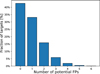Fig. 3 Distribution of the number of contaminants with ${\eta }_{\mathrm{k}}^{\mathrm{n}\mathrm{o}\mathrm{m}}>{\eta }_{min}$ for the targets in the magnitude range 10 ≤ P ≤ 13 from the catalog described in Sect. 5 and observed with 24 cameras.

7 Results

We present the results for the scenario described in Sect. 5.2. We analyze how variable EB transit parameters affect FP detection efficiency and resource allocation for the metrics described in this work.

7.1 Contamination landscape

The metrics and procedures described on Sect. 6 estimates the number of FPs per window. Fig. 3 shows the distribution of N_FP, Eq. (41), for targets in the magnitude range 10 ≤ P ≤ 13 from the stellar sample described in Sect. 5.1. We select this magnitude range because the brightest P5 targets will have their photometry extracted on-ground. Our results indicate that ~40% of the P5 targets have no contaminant stars capable of creating an FP, while ~35% have only one. This suggests that for more than 70% of the P5 targets only up to one of such contaminants is able to create an FP. Additionally, ~15% of the targets could have two contaminant stars causing FPs. The percentage of targets that can have more than two FPs is only of ~6%. This is the reason behind the simplification made in Sect. 6, i.e., the use of N_C = 10 in Eq. (41).

We studied the number of unique mask shapes for the nominal, extended and secondary masks. This is important because the introduction of extended and secondary masks could increase the total number of mask shapes such that the allowed onboard limit of the mask shapes is reached. In more detail, the onboard software has a mask library that consists of 8000 different shapes that are shared among the three types of masks. This library is prepared on-ground and it is programmed to be shared between the 24 N-CAMs. Fig. 4 shows the cumulative number of unique masks for the extended, nominal and secondary masks. The total number of unique mask shapes is 1179. This is way below the 8000 threshold in the mask library.

7.2 Efficiency of the metrics

Figures 5a and 5b show the results for the efficiency of centroid shift and flux measurements using nominal and double-aperture photometry. To produce these plots, we divided the target magnitude range (10 ≤ P ≤ 13) into 7 magnitude bins of 0.5 magnitudes in size.

For each bin, we randomly select 1000 targets from all available stars within the range P ± 0.25 magnitudes around each central value. Each data point represents the efficiency calculated for all 1000 targets within that specific magnitude bin. Also, all magnitude values referenced in the efficiency plots and tables correspond to target star magnitudes, including for secondary mask analyses. While secondary masks are centered on the most significant contaminant star, the efficiency is evaluated as a function of target magnitude to maintain consistency across all detection methods and to align with the magnitude-binned target selection approach described in Sect. 6.

Both Figures show a light blue and purple regions that overlap each other in the magnitude range 10.7 ≤ P ≤ 11.7. The light blue ones show the magnitude region where Earth-like planets can be detected by PLATO using 24 cameras. The light purple regions show the magnitude range where photometry extraction is expected to be performed on board. The region where they overlap is a rough estimate of where, in principle, PLATO could detect Earth-like planets with onboard photometry using 24 cameras. The P = 10.7 (i.e., V = 11 for a star with T_eff = 6000 K) threshold can be found in both the PLATO Red Book (2017) and ESA (2021). On the other hand, the P = 11.7 threshold is the result of the calculation presented in Appendix A, which confirms the results shown in Fig. 18 of Marchiori et al. (2019).

Figure 5a shows the efficiency of the centroid shift measurements using both nominal and double-aperture photometry. The calculations were performed for the cases of 24 and 6 cameras. The nominal centroids are very close in efficiency to the extended ones. The secondary centroid shifts are the next ones in efficiency. Since secondary masks are always centered on the most significant contaminant star of each window and if there is a transit happening on that contaminant star, the resulting centroid shift will be small. This means a less significant signal according to Eq. (40). We also notice a small decrease of their efficiency with increasing P magnitude. This can be explained showing the variation of the averaged centroid shift uncertainty, ${\sigma }_{\mathrm{k}}^{1\mathrm{h},{\mathrm{N}}_{\mathrm{T}}}$, of each metric with the magnitude. Fig. 6 shows this variation and we can see that the uncertainty associated with the extended centroid increases more rapidly than does the uncertainty associated with the nominal centroid. Hence, this explains the decrease of the efficiency with the magnitude.

Figure 5b shows the efficiency of flux measurements using the double-aperture photometry method. The calculations were performed again for both the cases of 24 and 6 cameras. The secondary flux is the most efficient method for both 24 and 6 cameras. This result is intuitive given that secondary masks are always centered on the contaminant with the highest probability to cause an FP in every window, given it has the highest SPR_k value and – in most cases – lowest NSR too.

We observe that efficiency is consistently higher for 24 cameras than for 6 cameras across all detection methods. This occurs because photometric uncertainty scales as $\sigma \propto 1/\sqrt{{\mathrm{N}}_{\mathrm{T}}}$ for both centroid and flux measurements, where N_T is the number of contributing cameras. Therefore, increasing from 6 to 24 cameras reduces uncertainty by a factor of $\sqrt{24/6}=2$, correspondingly increasing statistical significance by the same factor. A detailed analysis is provided in Appendix C using the extended flux as example.

Table 2 shows the magnitude-averaged efficiencies across the entire P5 range of the values in Figures 5a and 5b.

The results present in Table 2 show that secondary flux is the most efficient metric for detecting FPs. It is followed by the centroid shift measurements and finally by the extended flux. Secondary flux is particularly effective when only one contaminant is capable of generating an FP, as secondary masks are specifically designed for single-contaminant scenarios. However, when multiple contaminants can generate FPs, nominal and extended centroids become preferable due to their ability to simultaneously monitor several contaminants and their higher efficiency compared to extended flux, though only where computational resources allow it. Furthermore, flux measurements involving double-aperture photometry are both CPU and telemetry cheaper than centroid shift measurements computed with a nominal, secondary, or extended mask. This is because flux measurements require only a single scalar value per aperture, while centroid measurements must compute and transmit both x and y coordinates. Taken together, these considerations suggest that for the targets where flux measurements are as efficient as centroid shift measurements, the former should be preferred over the latter. More detailed suggestions about this are given in Sect. 8.2.

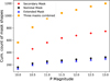Fig. 4 Cumulative count of unique mask shapes as a function of target P magnitude. The plot shows the unique number of each mask, i.e., extended (blue triangles), secondary (red crosses), and nominal (black circles), and the three types of masks together (orange squares).

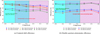Fig. 5 Comparison of centroid shifts and flux measurements with double-aperture photometry for detecting FPs. The results are produced for the case of variable transit parameters for the EBs. On the left, we show the efficiency for centroid shift measurements using the three types of masks mentioned in this work so far. On the right, we show the efficiency for both the secondary and extended masks. Both figures were obtained using 24 and 6 cameras for each mask. The Earth-like planet detection region is colored in light blue. The vertical dot-dashed red line corresponds to the P = 10.7 magnitude threshold. The pink colored region is the region where light curves will be produced on board for the P5 sample. The threshold of P = 11.7 is the vertical dashed green line.

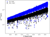Fig. 6 Distribution of the average uncertainty of the centroid shift (Eq. (37)) along target P magnitude for the extended (blue triangles) and nominal (black circles) masks.

8 Discussion and conclusions

8.1 Overall efficiency of the different metrics

As discussed in the previous sections, the efficiency of the different metrics depends on the conditions under which they are evaluated (see Sect. 6). These conditions are related to how PLATO measurements are obtained. Any change in the conditions will create changes in the efficiency of the metrics. An illustrative example is given by the extended flux measurements: if we replace the condition (${\delta }_{\mathrm{k}}^{\text{ext}}>{\delta }_{\mathrm{k}}^{\text{nom}}+3{\sigma }_{\delta }$) by the condition (${\delta }_{\mathrm{k}}^{\text{ext}}>{\delta }_{\mathrm{k}}^{\text{nom}}$) we get an efficiency for the extended flux of: 87.2%. As pointed out in Sect. 6.1.1, in the expression for σ_δ given by Eq. (43), we have assumed that the analysis of both the extended and nominal flux are done independently. A differential analysis of the extended flux and the nominal flux, as mentioned in the same Section, is expected to substantially reduce σ_δ and make the detection of FPs with the extended flux more efficient. Indeed, in the limit case where σ_δ tends to zero, the condition ${\delta }_{\mathrm{k}}^{\text{ext}}>{\delta }_{\mathrm{k}}^{\text{nom}}+3{\sigma }_{\delta }$ tends to the condition ${\delta }_{\mathrm{k}}^{\text{ext}}>{\delta }_{\mathrm{k}}^{\text{nom}}$. Hence, a differential analysis should increase the efficiency of the extended flux and put the latter somewhere between 73.5% and 87.2%. However, it should be noted that a differential analysis would require dedicated processing to be implemented on ground, which is not currently planned for the PLATO Exoplanet Analysis System (EAS).

8.2 Overall strategy for selecting the best metrics

Just after the secondary flux, the extended and nominal centroid measurements are the most efficient method for detecting FPs. However, the maximum number of centroids that can be measured on board is limited due to the CPU, memory and telemetry constrains. Indeed, we have the following onboard constraints (the numbers below are given for a single camera):

• Max. number of nominal centroids per camera: 7400.

• Max. number of extended centroids per camera: 7400.

• Max. number of extended or secondary flux per camera: 45 400.

• Max. number of nominal flux per camera: 104 850⁷.

Within these limits, it is possible to consider an optimal distribution between centroid measurements and extended or secondary flux measurements. To determine this distribution, we isolate the cases in which one metric is able to detect an FP while another is not. We care about the number of targets per camera because this is how most CPU resources are organized in the pipeline.

We present the percentage of FPs detected by each metric in combination with the other ones. The following abbreviations were introduced for convenience: NCOB for nominal centroid shift measurements, ECOB for extended centroid shift measurements, EFX for extended flux measurements, SFX for secondary flux measurements and SCOB for secondary centroid shift measurements. Table 3 shows the percentage of FPs for the different combinations of extended and nominal mask-based methods. For these comparisons the first ten most significant contaminants in terms of SPR_k in each window were considered. Accordingly, Table 4 shows the FPs percentage detection among the combinations of secondary mask-based methods. For these comparisons only the most prominent contaminant in terms of SPR_k of each window was considered⁸.

Table 3 shows that extended and nominal centroid shifts detect a similar fraction of FPs. Nominal centroid shifts recover 17.4% of FPs missed by extended fluxes, while extended centroid shifts recover 13.9%. Conversely, extended fluxes identify 7.2% of FPs missed by nominal centroid shifts but only 0.3% of those missed by extended centroid shifts. These results highlight the strong complementarity between extended fluxes and both extended and nominal centroid shifts. Accordingly, the choice between the extended centroids, nominal centroids and extended fluxes have to be made such as to optimize both the CPU and TM resources and the amount of FPs potentially detectable for each given target. However, extended fluxes could be prioritized since they have a lower cost in CPU and TM; also, nominal centroids could be prioritized over the extended centroids because they can be directly implemented in a window without invoking an additional, extended aperture. Table 4 shows that secondary flux clearly outperforms secondary centroids, detecting 20.6% of FPs that secondary centroids cannot identify, while secondary centroids detect only 3.9% of FPs missed by secondary flux. This demonstrates the greater superiority of flux-based over centroid-based detection when focusing on the most problematic contaminant. Together with the multi-contaminant comparison above, these results highlight the complementarity of flux- and centroid-based metrics, and how their usefulness depends on the context of each window and the available CPU and TM resources.

At this point, we can outline our proposed strategy to select the best metric for each target since this is how metrics will be assigned on ground (per target). The strategy takes into account the number of contaminants able to create a FP in each window, N_FP, as well as the results and computations presented so far. The strategy is summarized as follows:

• N_FP ≥ 2: For each target, we chose the extended flux, the nominal centroid metrics, or the extended centroid metrics based on which metric detects the largest number of FPs. If for a target the extended flux is able to detect the same number of FPs than the centroids, we choose the former because of its lower cost; otherwise we select the nominal centroid and, if needed, the extended centroid.

• N_FP = 1: We chose between the secondary flux and the nominal centroid. When for a given target the FP is detectable by the secondary flux (i.e., if the condition of Eq. (57) is verified), we select this metric because of its lower cost; otherwise, we select the centroid metric.

• N_FP = 0: Our proposal is to choose – if the resources allow it – an extended flux by default. This is because we might have missed some contaminant stars or we may have incorrect information about them. By choosing an extended flux by default we further maximize our chances of detecting an FP.

Table 5 summarizes the previous list.

8.3 An example of metric assignment

To assign a metric to a target we have to take into account for limitations imposed by the onboard software or the TM budget. At the same time, it has to take the scientific requirements into account as well. For instance the number of P5 targets for which photometry can be extracted on board is 80 000 for a single N-CAM. At the same time, centroid computations are limited to 14 800 targets per N-CAM while the number of extended/secondary flux to 45 400 targets again for a single N-CAM.

Table 6 shows our summarized proposed metric assignment scenario. To build it, we proceeded as follows: From Fig. 3 we see that the number of P5 targets with N_FP = 1 is ~35%, which corresponds to about 28 000 targets for a single N-CAM. Given that the efficiency of the secondary mask is 92%, we consider a secondary mask for the 92% of the 28 000 targets for a single N-CAM, these are about 25 760 targets. These are the targets that shall have a secondary flux computed on board, whereas for the remaining ~2240 stars, a nominal centroid measurement shall be considered. These values correspond to the N_FP = 1 row in Table 6. Furthermore, Fig. 3 shows that among the P5 sample, ~22% are expected to have N_FP ≥ 2; this represents a total of ~17 600 targets for a single N-CAM. These targets in principle can be monitored with extended flux measurements or nominal or extended centroid shift measurements. We can use Table 3 to find a possible share between metrics. According to it, extended centroid shifts detect 7.6% of the FPs missed by nominal centroids, while nominal centroids detect 17.4% of the FPs not detectable by extended fluxes. Therefore, we can start by assigning an extend centroid to 1337 targets (7.6% of 17 600) for which N_FP ≥ 2. Then, we can assign a nominal centroid to 2829 targets ((17 600–1337) × 0.174). Lastly, the remaining targets can get an extended flux, that is 13400 targets (17 600–1337–2829). These values correspond to the N_FP > 2 row of Table 6. We recall that the total centroid budget for a single N-CAM is up to 14 800 (7400 nominal plus 7400 extended). Finally, we can say that the maximum number of extended/secondary flux measurements (45 400) together with the maximum number of centroid measurements (14 800) fully suffices for all the targets for which N_FP > 0. The remaining number of extended flux measurements (6396 of the 45 400) can be assigned to the remaining P5 targets for which N_FP = 0 (the ~40% of the P5 sample); these targets can for instance be selected by putting more priority to the brightest ones. This gives the N_FP = 0 row in the Table 6. To conclude, this metrics share results in an optimal use of the resources while fulfilling the technical constraints: we have 25 760 secondary flux, 19830 extended flux and 6433 centroid measurements leading to a total of 52 023 targets, staying within the 80 000 targets for a single N-CAM budget, as summarized in the last row of Table 6.

8.4 Concluding remarks

In this paper, we have evaluated the efficiency of double-aperture photometry for detecting FPs. With this new method, we produced flux measurements that we compared with the known centroid shift method in terms of FP detection. The secondary flux was shown to be the most efficient metric overall, and it is followed in efficiency by extended centroid shifts, then by the nominal centroids, and then by the secondary centroid shifts. The extended flux is the last metric in terms of overall efficiency. However, we showed that for a higher fraction of the PLATO P5 targets, flux measurements using the double-aperture photometry are an alternative that is more competitive in terms of CPU and memory resources than the centroid shift method. We then established a strategy to optimally detect FPs with the double-aperture photometry and centroid methods while taking into account the technical limitations of the PLATO software and hardware. Finally, we conclude that by using the double-aperture photometry approach alongside centroid shift measurements implemented on board, a high fraction of FPs are expected to be discarded for the PLATO P5 sample. Our approach can also be used as a guideline for the design of future space missions aimed at detecting exoplanets with the transit technique.

As a next step, we plan on undertaking a future work involving a differential analysis for extended and nominal masks. Furthermore, we think another natural step is to analyze the dependence of our results regarding the following aspects: different FoV, camera pointings, and color-dependency of the targets and contaminants. However, we refer to the work by Gutierrez Canales (2025)⁹ for a detailed analysis of the efficiency of the metrics under different values of PSF temperature, diffusion kernel, and other configurations. Finally, a possible improvement for extended masks could consist of computing them in such a manner as to maximize the significance (for both extended flux and extended centroid shift measurements) of all the contaminant stars that can potentially generate a background transit. The exact procedure to obtain such optimal extended masks, however, needs to be studied in the future.

Acknowledgements

This work presents results from the European Space Agency (ESA) space mission PLATO. The PLATO payload, the PLATO Ground Segment and PLATO data processing are joint developments of ESA and the PLATO Mission Consortium (PMC). Funding for the PMC is provided at national levels, in particular by countries participating in the PLATO Multilateral Agreement (Austria, Belgium, Czech Republic, Denmark, France, Germany, Italy, Netherlands, Portugal, Spain, Sweden, Switzerland, Norway, and United Kingdom) and institutions from Brazil. Members of the PLATO Consortium can be found at https://platomission.com/. The ESA PLATO mission website is https://www.cosmos.esa.int/plato. We thank the teams working for PLATO for all their work. This work has benefited from financial support by Centre National d’Etudes Spatiales (CNES) in the framework of its contribution to the PLATO mission. FGC thanks the CNES and the Max Planck Institut für Sonnensystemforschung for its financial support during his PhD program. This work was supported in part by the German space agency (Deutsches Zentrum für Luftund Raumfahrt) under PLATO grant 50OP1902. This research has made use of astropy (see Astropy Collaboration 2022). FGC thanks Jesper Schou for his valuable comments and help, specially regarding the error bars in the efficiency plots. FGC also thanks Matthias Ammler-von Eiff and René Heller for their valuable comments and Ilyas Kuhlemann for his valuable help in the python code.

References

Appendix A Planets detectability

Although the main interest behind PLATO mission is to discover Earth-like planets, the mission is capable of detecting different types of planets as well. In this section, we are interested in studying the ability of PLATO to detect three different types of planets: Jovian, Super-Earths, and Earth-like planets. Fig. A.1 shows our results for each one of these planets. The results were produced taking into account n_tr = 3.

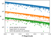Fig. A.1 Statistical significance of true planets (Eq. (22)), for three different types. The results are computed for 10000 targets in total. The dashed red line refers to the value of the detection threshold ηmin. The blue diamonds refer to the significance values related to Jovian planets using six cameras (δp = 10100 ppm and td = 29.6 hr), the orange stars refer to Super-Earths using six cameras (δp = 522 ppm and td = 42 hr), and the green circles refer to Earth-like planets using 24 cameras (δp = 84 ppm and td = 13 hr). The chosen δp and td values for the Jovian and Earth-like planets come from Fig. 18 from Marchiori et al. (2019). The chosen δp and td values for the Super-Earths were estimated interpolating between the Earth and Neptune values reported in Table 1 from Borucki et al. (1996).

Our analysis show that the significance of Earth-like planets around Sun-like stars has a magnitude limit at P~11.7, using N_T = 24 and n_tr = 3. This is consistent with the results provided by Fig. 18 from Marchiori et al. (2019). Another consistent result from Fig. A.1 is that PLATO is able to detect Jovian planets even if only using N_T = 6. In the case of Super-Earths, there was no previous analysis by Marchiori et al. (2019), but our results show as well that only using N_T = 6 could be enough for PLATO to detect Super-Earths since they appear to be well above the detectability threshold η_min when using 6 cameras.

Appendix B Nominal mask computation

The NSR expression useful to obtain the nominal mask is Eq. (36) from Marchiori et al. (2019): $${\mathrm{N}\mathrm{S}\mathrm{R}}_{\mathrm{n}}=\frac{\sqrt{{\mathrm{I}}_{\mathrm{n}}^{\mathrm{T}}+\sum _{\mathrm{k}=1}^{{\mathrm{N}}_{\mathrm{C}}}{\mathrm{I}}_{\mathrm{n}}^{\mathrm{k}}+\mathrm{B}\mathrm{\Delta }{\mathrm{t}}_{\exp }+{\sigma }_{\mathrm{D}}^2+{\sigma }_{\mathrm{Q}}^2}}{{\mathrm{I}}_{\mathrm{n}}^{\mathrm{T}}}.$$(B.1)

The terms used in Eq. (B.1) are defined in Table 1 since they are the same than the ones from Eq. (3). The subscript “n” indicates that we compute the NSR for every window pixel. Once we computed it for 36 pixels of the window, we sort them in increasing order. We use the subscript “m” for denoting the index of the sorted window pixels. These pixels are used to compute what Marchiori et al. (2019) called the “aggregate NSR,” which is written as $${\mathrm{N}\mathrm{S}\mathrm{R}}_{\text{agg}}(\mathrm{m})=\frac{\sqrt{\sum _{\mathrm{n}=1}^{\mathrm{m}}({\mathrm{I}}_{\mathrm{n}}^{\mathrm{T}}+\sum _{\mathrm{k}=1}^{{\mathrm{N}}_{\mathrm{C}}}{\mathrm{I}}_{\mathrm{n}}^{\mathrm{k}}+\mathrm{B}\mathrm{\Delta }{\mathrm{t}}_{\text{exp\hspace{0.17em}}}+{\sigma }_{\mathrm{D}}^2+{\sigma }_{\mathrm{Q}}^2)}}{\sum _{\mathrm{n}=1}^{\mathrm{m}}{\mathrm{I}}_{\mathrm{n}}^{\mathrm{T}}}.$$(B.2)

Finally, we obtained the nominal mask, ω_n, by looking for the collection of pixels that minimizes Eq. (B.2). This is shown in Figs. 13 and 14c of Marchiori et al. (2019) and in Figs. B.1a and B.1b of this work. This refers to a star with P = 11.12.

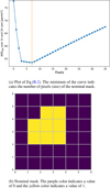Fig. B.1 Top: Example of NSR plot. Bottom: Consequent shape of the nominal mask. For this case, the size of the nominal mask is 8 pixels.

The way for building a secondary mask is completely analogous to what have just been described. The only difference is that we substitute ${\mathrm{I}}_{\mathrm{n}}^{\mathrm{T}}$ by ${\mathrm{I}}_{\mathrm{n}}^{\mathrm{k}\mathrm{m}\mathrm{a}\mathrm{x}}$ since for the secondary mask the star with the highest SPR value in the window is regarded as the target. Furthermore, the way of building the extended mask is simply by surrounding the nominal mask by a single pix. Fig. B.2 shows the average size in pixels of the three types of masks as a function of the P target magnitude.

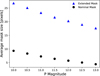Fig. B.2 Average mask size in pixels for the nominal (black circles) and extended (blue triangles) masks as a function of the target P magnitude.

Appendix C Change in efficiency when switching from 24 to 6 cameras

To investigate the change in efficiency of both double-aperture photometry and centroid shifts when shifting from 24 to 6 cameras, we use the extended mask as an example. The analysis for other versions of both methods is analogous. We begin with the following expression involving N_FP and ${\mathrm{N}}_{\mathrm{F}\mathrm{P}}^{\text{ext}}$ for both 24 and 6 cameras: $$\frac{{\mathrm{N}}_{\mathrm{F}\mathrm{P}}^{\text{ext,}6\text{cameras}}}{{\mathrm{N}}_{\mathrm{F}\mathrm{P}}^{6\text{cameras}}}=\frac{{\mathrm{N}}_{\mathrm{F}\mathrm{P}}^{\text{ext,24cameras}}}{{\mathrm{N}}_{\mathrm{F}\mathrm{P}}^{24\text{cameras}}}\left[\frac{(1-\alpha )}{(1-\beta )}\right],$$(C.1)

where α and β are terms useful for investigating the efficiency change with different camera numbers. This change results from the loss of a certain number of stars when switching the camera number. We denote this loss as Loss^ext, defined as $${\mathrm{Loss}}^{\mathrm{e}\mathrm{x}\mathrm{t}}=\alpha {\mathrm{N}}_{\mathrm{F}\mathrm{P}}^{\mathrm{e}\mathrm{x}\mathrm{t},24\text{cameras}}.$$(C.2)

We observe that switching from 6 to 24 cameras can double the signal. The efficiency change can be attributed to the distribution change of ${\eta }_{\mathrm{k}}^{\text{ext}}$ (denoted as L₁), the distribution change of ${\eta }_{\mathrm{k}}^{\mathrm{n}\mathrm{o}\mathrm{m}}$ (denoted as L₂), or a combination of both (L₁ + L₂). Additionally, the efficiency change might depend on the denominator, the distribution change of ${\eta }_{\mathrm{k}}^{\text{nom}}$ (denoted as L₂). This is expressed by $$\begin{array}{rl}& {\mathrm{L}}_1=({\eta }_{min}<{\eta }_{\mathrm{k}}^{\mathrm{e}\mathrm{x}\mathrm{t}}<2{\eta }_{min})\wedge ({\eta }_{\mathrm{k}}^{\mathrm{n}\mathrm{o}\mathrm{m}}<2{\eta }_{min}),\\ & {\mathrm{L}}_2=({\eta }_{min}<{\eta }_{\mathrm{k}}^{\mathrm{n}\mathrm{o}\mathrm{m}}<2{\eta }_{min})\wedge ({\eta }_{\mathrm{k}}^{\mathrm{e}\mathrm{x}\mathrm{t}}<2{\eta }_{min}),\\ & {\mathrm{L}}_3={\mathrm{L}}_1+{\mathrm{L}}_2,\\ & {\mathrm{L}}_4=({\eta }_{min}<{\eta }_{\mathrm{k}}^{\mathrm{n}\mathrm{o}\mathrm{m}}<2{\eta }_{min}).\end{array}$$(C.3)

Then equation (C.2) becomes $$\begin{array}{rl}{\mathrm{Loss}}^{\mathrm{e}\mathrm{x}\mathrm{t}}=& \alpha {\mathrm{N}}_{\mathrm{F}\mathrm{P}}^{\mathrm{e}\mathrm{x}\mathrm{t},24\text{cameras}}=\sum _{\text{targets}}\sum _{\mathrm{k}=1}^{{\mathrm{N}}_{\mathrm{C}}}({\delta }_{\mathrm{k}}^{\mathrm{e}\mathrm{x}\mathrm{t}}>{\delta }_{\mathrm{k}}^{\mathrm{n}\mathrm{o}\mathrm{m}})\times \\ & \left[{\mathrm{L}}_1\text{\hspace{0.17em}or\hspace{0.17em}}{\mathrm{L}}_2\text{\hspace{0.17em}or\hspace{0.17em}}{\mathrm{L}}_3\text{\hspace{0.17em}and\hspace{0.17em}}{\mathrm{L}}_4\right].\end{array}$$(C.4)

We then obtained the values for L₁, L₂, L₃, and L₄. From equation C.4 we derived $$\alpha =\frac{{\mathrm{L}}_1+{\mathrm{L}}_2+{\mathrm{L}}_3}{{\mathrm{N}}_{\mathrm{F}\mathrm{P}}^{\mathrm{e}\mathrm{x}\mathrm{t},24\text{cameras}}},$$(C.5)

and $$\beta =\frac{{\mathrm{L}}_4}{{\mathrm{N}}_{\mathrm{F}\mathrm{P}}^{\text{ext,24cameras\hspace{0.17em}}}}.$$(C.6)

Our analysis shows that (1 − α) is always greater than (1 − β)

Appendix D Reference table

With the aim to make our results as reproducible as possible, the interested reader can have Table D.1 as reference. Table D.1 shows the most relevant metrics for a given target in our stellar sample and the ten most significant contaminants around it.

All Tables

All Figures

Fig. 1 Schematic view (from left to right) of example nominal, extended, and secondary masks. For the extended and secondary masks, the respective nominal mask is represented with dashed lines. In this case, the nominal mask consists of 5 pixels, the extended mask has 19 pixels, and the secondary mask has 3 pixels. The red circle represents the target star, and the cyan triangle represents a nearby contaminant star that could be an EB. Nominal masks are used to extract target photometry and were built to have the lowest NSR. The extended masks are constructed by enlarging the nominal masks, typically by surrounding each nominal mask with a ring of one pixel. Secondary masks are typically smaller and are centered on the most problematic contaminant star in the window.

In the text

Fig. 2 Simulated PLATO PSFs (1/64 pixel resolution) at different angular positions, α, of a flux source in the FoV of a PLATO camera. When α = 0° the source is in the center of the FoV and when α = 18° the source is at the edge of the FoV. The top row shows the PSFs without charge diffusion, while in the middle row a Gaussian kernel was applied to simulate charge diffusion in the CCD. The bottom row shows the PSF integrated over the pixels of a 6x6 window. The color scheme goes from the highest value (red) to the smallest values (blue).

In the text

	Fig. 3 Distribution of the number of contaminants with ${\eta }_{\mathrm{k}}^{\mathrm{n}\mathrm{o}\mathrm{m}}>{\eta }_{min}$ for the targets in the magnitude range 10 ≤ P ≤ 13 from the catalog described in Sect. 5 and observed with 24 cameras.
In the text

	Fig. 4 Cumulative count of unique mask shapes as a function of target P magnitude. The plot shows the unique number of each mask, i.e., extended (blue triangles), secondary (red crosses), and nominal (black circles), and the three types of masks together (orange squares).
In the text

Fig. 5 Comparison of centroid shifts and flux measurements with double-aperture photometry for detecting FPs. The results are produced for the case of variable transit parameters for the EBs. On the left, we show the efficiency for centroid shift measurements using the three types of masks mentioned in this work so far. On the right, we show the efficiency for both the secondary and extended masks. Both figures were obtained using 24 and 6 cameras for each mask. The Earth-like planet detection region is colored in light blue. The vertical dot-dashed red line corresponds to the P = 10.7 magnitude threshold. The pink colored region is the region where light curves will be produced on board for the P5 sample. The threshold of P = 11.7 is the vertical dashed green line.

In the text

	Fig. 6 Distribution of the average uncertainty of the centroid shift (Eq. (37)) along target P magnitude for the extended (blue triangles) and nominal (black circles) masks.
In the text

Fig. A.1 Statistical significance of true planets (Eq. (22)), for three different types. The results are computed for 10000 targets in total. The dashed red line refers to the value of the detection threshold ηmin. The blue diamonds refer to the significance values related to Jovian planets using six cameras (δp = 10100 ppm and td = 29.6 hr), the orange stars refer to Super-Earths using six cameras (δp = 522 ppm and td = 42 hr), and the green circles refer to Earth-like planets using 24 cameras (δp = 84 ppm and td = 13 hr). The chosen δp and td values for the Jovian and Earth-like planets come from Fig. 18 from Marchiori et al. (2019). The chosen δp and td values for the Super-Earths were estimated interpolating between the Earth and Neptune values reported in Table 1 from Borucki et al. (1996).

In the text

	Fig. B.1 Top: Example of NSR plot. Bottom: Consequent shape of the nominal mask. For this case, the size of the nominal mask is 8 pixels.
In the text

	Fig. B.2 Average mask size in pixels for the nominal (black circles) and extended (blue triangles) masks as a function of the target P magnitude.
In the text

References

- Astropy Collaboration (Price-Whelan, A. M., et al.) 2022, ApJ, 935, 167 [NASA ADS] [CrossRef] [Google Scholar]
- Auvergne, M., Bodin, P., Boisnard, L., et al. 2009, A&A, 506, 411 [NASA ADS] [CrossRef] [EDP Sciences] [Google Scholar]
- Batalha, N. M., Rowe, J. F., Gilliland, R. L., et al. 2010, ApJ, 713, L103 [NASA ADS] [CrossRef] [Google Scholar]
- Börner, A., Paproth, C., Cabrera, J., et al. 2024, Exp. Astron., 58, 1 [CrossRef] [Google Scholar]
- Borucki, W. J., Dunham, E. W., Koch, D. G., et al. 1996, Astrophys. Space Sci., 241, 111 [Google Scholar]
- Borucki, W., Koch, D., Basri, G., et al. 2007, Proc. Int. Astron. Union, 3, 17 [NASA ADS] [CrossRef] [Google Scholar]
- Borucki, W. J., Koch, D., Basri, G., et al. 2010, Science, 327, 977 [Google Scholar]
- Bray, J. C., Kolb, U., Rowden, P., et al. 2023, MNRAS, 518, 3637 [Google Scholar]
- Bryson, S. T., Jenkins, J. M., Gilliland, R. L., et al. 2013, PASP, 125, 889 [NASA ADS] [CrossRef] [Google Scholar]
- Bryson, S., Coughlin, J., Batalha, N. M., et al. 2020, AJ, 159, 279 [NASA ADS] [CrossRef] [Google Scholar]
- Cabrera, J., Barros, S. C. C., Armstrong, D., et al. 2017, A&A, 606, A75 [NASA ADS] [CrossRef] [EDP Sciences] [Google Scholar]
- Christiansen, J. L., Clarke, B. D., Burke, C. J., et al. 2020, AJ, 160, 159 [NASA ADS] [CrossRef] [Google Scholar]
- Díaz, R. F., Almenara, J. M., Santerne, A., et al. 2014, MNRAS, 441, 983 [Google Scholar]
- ESA. 2021, PLATO Science Requirements Document [Google Scholar]
- Gaia Collaboration (Prusti, T., et al.) 2016, A&A, 595, A1 [NASA ADS] [CrossRef] [EDP Sciences] [Google Scholar]
- Gaia Collaboration (Vallenari, A., et al.) 2023, A&A, 674, A1 [NASA ADS] [CrossRef] [EDP Sciences] [Google Scholar]
- Goupil, M. J., Catala, C., Samadi, R., et al. 2024, A&A, 683, A78 [NASA ADS] [CrossRef] [EDP Sciences] [Google Scholar]
- Günther, M. N., Queloz, D., Gillen, E., et al. 2017, MNRAS, 472, 295 [Google Scholar]
- Gutierrez Canales, C. F. 2025, Theses, Université Paris sciences et lettres; Max-Planck-Institut für Sonnensystemforschung [Google Scholar]
- Hedges, C. 2021, RNNAS, 5, 262 [Google Scholar]
- Heller, R., Harre, J.-V., & Samadi, R. 2022, A&A, 665, A11 [NASA ADS] [CrossRef] [EDP Sciences] [Google Scholar]
- Hsu, D. C., Ford, E. B., Ragozzine, D., & Morehead, R. C. 2018, AJ, 155, 205 [NASA ADS] [CrossRef] [Google Scholar]
- Jenkins, J. M., Caldwell, D. A., Chandrasekaran, H., et al. 2010, ApJ, 713, L120 [Google Scholar]
- Kirk, B., Conroy, K., Prša, A., et al. 2016, AJ, 151, 68 [Google Scholar]
- Kunimoto, M., & Matthews, J. M. 2020, AJ, 159, 248 [NASA ADS] [CrossRef] [Google Scholar]
- Lissauer, J. J., Marcy, G. W., Rowe, J. F., et al. 2012, ApJ, 750, 112 [NASA ADS] [CrossRef] [Google Scholar]
- Marchiori, V. 2019, PhD thesis, LESIA, Paris Observatory, France, thèse de doctorat dirigée par Samadi, Réza David et Oliveira Fialho, Fabio de Astronomie et Astrophysique, Paris Sciences et Lettres (ComUE) [Google Scholar]
- Marchiori, V., Samadi, R., Fialho, F., et al. 2019, A&A, 627, A71 [NASA ADS] [CrossRef] [EDP Sciences] [Google Scholar]
- Melton, E. J., Feigelson, E. D., Montalto, M., et al. 2024, AJ, 167, 203 [NASA ADS] [CrossRef] [Google Scholar]
- Montalto, M., Piotto, G., Marrese, P. M., et al. 2021a, A&A, 653, A98 [NASA ADS] [CrossRef] [EDP Sciences] [Google Scholar]
- Montalto, M., Piotto, G., et al. 2021b, A&A, 653, A98 [NASA ADS] [CrossRef] [EDP Sciences] [Google Scholar]
- Mowlavi, N., Holl, B., Lecoeur-Taïbi, I., et al. 2023, A&A, 674, A16 [NASA ADS] [CrossRef] [EDP Sciences] [Google Scholar]
- Nascimbeni, V., Piotto, G., Börner, A., et al. 2022, A&A, 658, A31 [NASA ADS] [CrossRef] [EDP Sciences] [Google Scholar]
- Pertenais, M., Cabrera, J., Griessbach, D., et al. 2021a, SPIE Conf. Ser., 11852, 1185209 [NASA ADS] [Google Scholar]
- Pertenais, M., Cabrera, J., Paproth, C., et al. 2021b, SPIE Conf. Ser., 11852, 18524Y [Google Scholar]
- Prša, A., Batalha, N., Slawson, R. W., et al. 2011, AJ, 141, 83 [Google Scholar]
- Prša, A., Kochoska, A., Conroy, K. E., et al. 2022, ApJS, 258, 16 [CrossRef] [Google Scholar]
- Rauer, H., & Heras, A. M. 2018, Space Missions for Exoplanet Science: PLATO, eds. H. J. Deeg & J. A. Belmonte (Cham: Springer International Publishing), 1309 [Google Scholar]
- Rauer, H., Catala, C., Aerts, C., et al. 2014, Exp. Astron., 38, 249 [Google Scholar]
- Rauer, H., Aerts, C., Cabrera, J., et al. 2025, Exp. Astron., 59, 26 [Google Scholar]
- Ricker, G. R., Winn, J. N., Vanderspek, R., et al. 2015, J. Astron. Telesc. Instrum. Syst., 1, 014003 [Google Scholar]
- Samadi, R., Deru, A., Reese, D., et al. 2019, A&A, 624, A117 [NASA ADS] [CrossRef] [EDP Sciences] [Google Scholar]
- Söderhjelm, S., & Dischler, J. 2005, A&A, 442, 1003 [NASA ADS] [CrossRef] [EDP Sciences] [Google Scholar]
- Torres, G., Fressin, F., Batalha, N. M., et al. 2011, ApJ, 727, 24 [NASA ADS] [CrossRef] [Google Scholar]
- Ziemke, C., Grießbach, D., Eising, J., et al. 2023, in 2023 European Data Handling & Data Processing Conference (EDHPC), 1 [Google Scholar]
As of 29 July 2025 from the NASA Exoplanet Archive.
The introduction present in Melton et al. (2024) shows an extensive list of papers regarding the vetting of exoplanet candidates from transit signals.
It requires only one measurement per imagette for flux and two for centroid computations (x and y positions) per imagette.
This estimation is ~50% higher than another, previous one produced with Hipparcos data. The authors suggest that the increase is due to Kepler’s photometric superiority.
This number includes the stars from the guest observer program, that is about 20 000 targets per camera and for a single pointing.
The fractions of FP detection were computed by considering the proportion of contaminant stars that meet the detection criteria for each metric described in Sect. 6 in each magnitude bin. These fractions were then weighted based on the actual distribution of stars across magnitude bins, with error estimates derived from the weighted variance assuming a binomial distribution.
The thesis is available here: https://theses.hal.science/tel-05165095