| Issue |
A&A
Volume 707, March 2026
|
|
|---|---|---|
| Article Number | A291 | |
| Number of page(s) | 12 | |
| Section | Stellar structure and evolution | |
| DOI | https://doi.org/10.1051/0004-6361/202554366 | |
| Published online | 12 March 2026 | |
The impact of differential rotation on the stochastic excitation of acoustic modes in solar-like pulsators
1
Université Paris-Saclay, Université Paris Cité, CEA, CNRS, AIM, Gif-sur-Yvette F-91191, France
2
Université PSL, Paris 75006, France
★ Corresponding author: This email address is being protected from spambots. You need JavaScript enabled to view it.
Received:
4
March
2025
Accepted:
2
July
2025
Abstract
Context. Acoustic modes are excited by turbulent convection in the outer convective envelope of solar-like stars. Observational results from asteroseismic studies have shown that 44% of solar-like stars do not present detectable stochastically excited acoustic modes. This phenomenon appears to be related to their rotation rate and magnetic activity. Indeed, rotation locally modifies the properties of convection, which in turn influences the stochastic excitation of stellar oscillation modes. In a first paper, we showed that uniform rotation tends to diminish the mode amplitudes significantly. However, convective envelopes in solar-type stars differentially rotate, and the rotation rate difference between mid-latitudes and the equator can reach up to 60%, as shown by recent asteroseismic works.
Aims. In this paper, we examine the impact of differential rotation on the stochastic excitation of acoustic modes in solar-like stars.
Methods. We provide theoretical predictions for the excitation of acoustic modes in a differentially rotating solar-like star. We used rotating mixing length theory to model the local influence of differential rotation on convection. We then estimated the resulting impact on power injection by turbulent convection into oscillation modes numerically, using a combination of the MESA stellar structure and evolution code and GYRE stellar pulsation code.
Results. We show that the power injected in acoustic modes differs by up to 30% for stars with the same mean rotation rate (i.e. 5Ω⊙) but a distinct differential rotation rate. The excitation of axisymmetric acoustic modes is further inhibited in the anti-solar differential rotation regime, where the poles of stars rotate faster than their equators compared to the uniform rotation case. This could hinder mode detection in such configurations. In contrast, in solar differential rotation regimes, where the equator rotates faster than the poles, acoustic mode excitation is less inhibited compared to the uniform rotation case. We also studied the influence of the azimuthal order and show that the amplitudes can differ by up to 30% for modes with the same order, ℓ, and a different azimuthal order, m. The trends for sectoral modes (with |m|=l) is the opposite than the one observed for the axisymmetric modes.
Conclusions. This study permits a first prediction of the excitation of acoustic modes as a function of the differential rotation in solar-like pulsators. On the one hand, efficient mode excitation may enable the detection of rotational frequency splittings. On the other hand, weaker-than-expected or stronger-than-expected excitation compared to predictions based on uniform rotation could provide valuable hints into differential rotation. The results are crucial to interpret data from past and ongoing asteroseismic space missions, such as Kepler/K2 and TESS, and to prepare for PLATO.
Key words: asteroseismology / convection / turbulence / stars: oscillations / stars: rotation / stars: solar-type
G. Biscarrat and L. Bessila equally contributed to this work.
© The Authors 2026
 Open Access article, published by EDP Sciences, under the terms of the Creative Commons Attribution License (https://creativecommons.org/licenses/by/4.0), which permits unrestricted use, distribution, and reproduction in any medium, provided the original work is properly cited.
This article is published in open access under the Subscribe to Open model. This email address is being protected from spambots. You need JavaScript enabled to view it. to support open access publication.
1. Introduction
Acoustic modes are a powerful probe of stellar interiors (see the reviews on helioseismology and asteroseismology by Aerts et al. 2010; García & Ballot 2019; Christensen-Dalsgaard 2021). As pressure fluctuations lead to luminosity variations, acoustic oscillation modes have been observed at the surface of solar-like stars through photometric data (Michel et al. 2008; Chaplin et al. 2010; Huber et al. 2019) from space missions such as CoRoT (Convection, Rotation, and Transits, Baglin et al. 2006), Kepler/K2 (Borucki et al. 2008, 2010; Howell et al. 2014), and TESS (Transiting Exoplanet Survey Satellite, Ricker et al. 2014). Amplitudes of solar-like oscillations result from a balance between stochastic excitation due to turbulent convection (see e.g. Samadi & Goupil 2001) and damping (e.g. Grigahcène et al. 2005) near the surface of the outer convection zone. The driving mechanism has been investigated in many studies (Goldreich & Keeley 1977; Balmforth 1992; Samadi & Goupil 2001; Chaplin et al. 2005; Belkacem 2008), and it has been shown (see e.g. Samadi et al. 2005) that the main contribution driving the oscillations in solar-like pulsators is the Reynolds stresses source term due to turbulent convection.
However, acoustic modes are not detected in a large fraction of stars with a convective envelope and hence where stochastically excited oscillations would be expected (e.g. Chaplin et al. 2011). Mathur et al. (2019) studied a sample of 867 solar-like stars observed with the Kepler space mission and found that acoustic modes are detected in only 44% of the stars. This non-detection could result from high magnetic activity, rapid rotation, or other factors, such as metallicity or binarity. Including those physical phenomena in the theoretical modelling of stochastic excitation is therefore paramount.
When it comes to rotation, Belkacem et al. (2009) generalised the formalism by Samadi & Goupil (2001), taking into account the perturbation of acoustic modes due to uniform rotation. Previously, in Bessila et al. (2025), we introduced the direct impact of a uniform rotation on turbulent convection, which results in a diminution of the mode excitation rates for rapid rotation. To do so, we used the prescriptions of the rotating mixing length theory (R-MLT) to describe the modification of the rms velocity and scale of turbulent convection by rotation (e.g. Stevenson 1979; Augustson & Mathis 2019). This theory relies on the idea that the mode that maximises the heat transport is dominant in the convective flow according to Malkus (1954). The whole turbulent convective spectrum is then modelled by this single mode. Despite this simplification, R-MLT prescriptions have been successfully compared to 3D non-linear hydrodynamical numerical simulations in a Cartesian geometry in which the rotation axis is aligned with gravity (Barker et al. 2014). Next, Currie et al. (2020) computed the same type of Cartesian numerical simulations with a tilted rotation axis, allowing configurations representative of all latitudes in stars to be studied. Again, the prescriptions from Stevenson (1979) agree well with the results from numerical simulations and hold over several decades in Rossby numbers at most latitudes. However, as pointed out in Currie et al. (2020), this single-mode theory fails to capture the anisotropy of heat transport near the equator. In a previous work, we thus generalised the existing formalism of the stochastic excitation of stellar oscillation modes to include uniform rotation by taking into account the local modification of convection by rotation using R-MLT (Bessila et al. 2025). We showed that the resulting amplitude of acoustic modes can decrease by up to 70% for a 20Ω⊙ rotation rate when compared to the non-rotating case, in agreement with the observational tendency highlighted in Mathur et al. (2019).
In this article, we extend this formalism to include differential rotation (hereafter DR). Acoustic oscillations at the Sun’s surface detected using helioseismology have revealed its rotation profile in the convective zone (Chaplin et al. 1999; Schou et al. 1998; Thompson et al. 2003; Couvidat et al. 2003; García et al. 2007). The latitudinal DR rate between the poles and the equator in the convective envelope is nearly 30%, whereas the radiative core exhibits a solid-body rotation until 0.25 R⊙. Other ways exist to access information on the rotation of stars other than the Sun. For instance, spectroscopic measurements can estimate surface velocity and the related DR by observing the broadening of absorption lines caused by the Doppler effect (Donati & Cameron 1997; Barnes et al. 2005). The photometric variability of starspots at different latitudes can also be used (Oláh et al. 2009). More recently, significant progress has been made in detecting the magnitude of the latitudinal DR by analysing its impact on rotational frequency-splittings of mixed and acoustic modes (see e.g. Deheuvels et al. 2015; Benomar et al. 2015, 2018; Bazot et al. 2019). For example, Benomar et al. (2018) detected latitudinal DR in some solar-like stars, with a median value of 64% difference between mid-latitudes and the equator. The unexpectedly high values for the shear pose a challenge to understanding the angular momentum transport in the convective envelope of low-mass stars (e.g. Käpylä et al. 2014; Brun et al. 2022) and highlight that DR should not be neglected or treated as a small perturbation in theoretical models.
Characterising the DR in the convective envelope of solar-type stars is key, as it is one of the most important ingredients for dynamo action (e.g. Saar & Brandenburg 1999; Charbonneau 2005; Jouve et al. 2010; Brun & Browning 2017; Noraz et al. 2022a). For a given star, the DR profile is directly related to the dimensionless fluid Rossby number, ℛof (defined in Eq. 25), which quantifies the ratio between the inertia term and the Coriolis acceleration in the Navier-Stokes equation (see e.g. Gilman 1977; Gilman & Glatzmaier 1981; Matt et al. 2011; Guerrero et al. 2013; Gastine et al. 2013; Käpylä et al. 2014; Brun et al. 2017, 2022; Noraz et al. 2022a). Studies using direct numerical simulations have highlighted a change in the DR profile between intermediate and slow rotators. The transition between these two states occurs around ℛof = 1 in numerical simulations (Gastine et al. 2013; Käpylä et al. 2014; Karak et al. 2015; Brun et al. 2022). Intermediate rotators (0.15 ≲ ℛof ≲ 1) exhibit a solar-like conical DR characterized by a slow rotation at the poles and a faster rotation at the equator (e.g. Brun et al. 2017). In contrast, slow rotators (ℛof ≳ 1) are the seat of an anti-solar DR, with a slower equator and faster poles. Following these numerical results, Benomar et al. (2018) analysed the DR in 40 solar-like stars using asteroseismology and found that some stars could have an anti-solar DR profile. Doppler imaging spectroscopy has allowed for some other detections in subgiants and red giants stars (see e.g. Kovári et al. 2007). Noraz et al. (2022b) also identified main sequence stars potentially hosting anti-solar DR in the Kepler sample. Finally, several trends for the DR in solar-like stars have been uncovered by numerical simulations and observations: The DR ΔΩ appears to increase with the stellar mass. Numerical simulations have also revealed dependencies between the DR and the rotation: ΔΩ ∼ Ω★r, with r as a positive exponent between 0.2 and 0.7 (e.g. Reinhold & Reiners 2013). However, the exact value of the exponent r is still under investigation (e.g. Brun et al. 2022).
In this framework, we have demonstrated how a uniform rotation can impact the injection of energy by turbulent convection into acoustic modes propagating in solar-type stars (Bessila et al. 2025), and therefore their potentially strong DR must be taken into account. In this work, we aim to understand how acoustic mode amplitudes are affected by the DR of a star through the modification it induces on turbulent convection that in turn excites these modes. Since acoustic modes enable one to characterise the DR in the convective envelope of low-mass stars, it is indeed crucial to coherently predicting their excitation rate and amplitude. This knowledge then allows us to better constrain the observed DR, which is key to understanding magnetism and angular momentum redistribution in these regions. This paper is organised as follows: We present the theoretical model of acoustic mode excitation in a differentially rotating convective envelope in Section 2. We then implement the obtained theoretical prescriptions to estimate the energy injected into acoustic oscillation modes in a differentially rotating solar-type star modelled using the MESA and GYRE stellar modelling suite in Section 3. In Section 4 we explore the influence of stellar mass on DR and its subsequent effect on the excitation of acoustic modes. Finally, we present the key results of our study and discuss their implications for understanding observed acoustic mode amplitudes in differentially rotating solar-like stars in Section 5.
2. Turbulent stochastic excitation in differentially rotating stars
2.1. Differential rotation
Helioseismology has demonstrated that the Sun’s convective zone rotates nearly uniformly in the radial direction (see e.g. Schou et al. 1998; Thompson et al. 2003; García et al. 2007; Eff-Darwich & Korzennik 2013). In addition, stars exhibit different DR profiles depending on their evolutionary stage (Noraz et al. 2024). The DR profile is first mostly cylindrical during the pre-main sequence (when ℛof ≲ 0.15). During this phase, low-mass stars are fast rotators, and the Coriolis acceleration constrains the flows because of the Taylor-Proudman constraint (Proudman 1916; Taylor 1917). In this case, the local rotation rate depends on the distance to the rotation axis: Ω(r, θ) = Ω(r sin θ), where θ is the co-latitude and r is the radius (see e.g. Brun et al. 2017, 2022). During the main sequence, the DR becomes conical (when ℛof ≳ 0.15). The local rotation rate depends mainly on the co-latitude, as in the Sun, where the equator rotates faster than the poles. For more massive or evolved stars, the conical DR can become anti-solar if ℛof ≳ 1, with stellar poles rotating faster than the equator. As the Kepler observational sample is dominated by main sequence stars, we thus focus on a conical DR profile in this study in order to provide a tractable model that can easily be applied to a broad sample of stars. We modelled the rotation profile as follows:
 (1)
(1)
where Ωp is the rotation rate at the poles and ΔΩ ≡ Ωeq − Ωp is the difference between the rotation rate at the equator and the poles. If ΔΩ > 0, the rotation rate at the equator is higher than the one at the poles: It is a solar DR profile. On the contrary, if ΔΩ < 0, the rotation profile is anti-solar. As we aimed to compare the impact of DR to the uniformly rotating case, we defined the mean rotation rate over the convective zone as
 (2)
(2)
We then chose  as the reference rotation rate in our model.
According to the observational study by Benomar et al. (2018), the relative DR rate between the equator and mid-latitude can go up to (Ω45 − Ωeq)/Ωeq ∼ 0.6, which corresponds to  in our model, following Eqs. (1) and (2). For simplicity, we defined the relative DR rate as
 (3)
(3)
so that the DR profile writes
 (4)
(4)
We plot in Fig. 1 the conical DR profile, where we chose the solar value for the mean rotation rate:  nHz, where Ωeq, ⊙ and Ωp, ⊙ are the solar rotation rates at the equator and the poles, respectively.
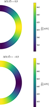 |
Fig. 1. Conical DR profile for a solar regime (top) and an anti-solar regime (bottom) following Eq. (1). In both cases, |

2.2. Excitation by turbulent convection
We build on the formalisms by Samadi & Goupil (2001), Belkacem et al. (2009), and Bessila et al. (2025). We only take into account the Reynolds stresses in the convective envelope as the source that drives the oscillation modes in the stellar cavity. Indeed, Samadi et al. (2007) showed that the entropy fluctuations account for only 10% of the total injected power, and Belkacem et al. (2009) demonstrated that the source terms coming from the Coriolis acceleration and the DR are negligible as well. Nonetheless, DR plays a role in locally modifying convective properties, thereby influencing the Reynolds stresses as a source term. By linearising Navier-Stokes and continuity equations and then separating the velocity due to the oscillations, uosc, from the one due to turbulent convection, Ut, we derived the forced wave equation (we refer the reader to Belkacem et al. 2009, for more details about this derivation):
 (5)
(5)
where ρ0 is the density, ℒ is the linear operator describing the propagation of waves, 𝒟 is the damping term, and ∂𝒞/∂t contains negligible source terms. The symbol 𝒮R is the Reynolds stresses source term defined as
![Mathematical equation: $$ \begin{aligned} \frac{\partial \mathcal{S} _R}{\partial t} = -\frac{\partial }{\partial t} \left[\nabla : \left(\rho _0 {\boldsymbol{U}}_{\rm t} {\boldsymbol{U}}_{\rm t}\right)\right], \end{aligned} $$](/articles/aa/full_html/2026/03/aa54366-25/aa54366-25-eq10.gif) (6)
(6)
which acts as the forcing for the waves.
The wave velocity field is related to the displacement by the expression
![Mathematical equation: $$ \begin{aligned} {\boldsymbol{u}}_{\rm osc} = A(t) \left[i\widehat{\omega } \boldsymbol{\xi }(\boldsymbol{r}) - (\boldsymbol{\xi }(\boldsymbol{r}) \cdot \nabla \boldsymbol{\Omega }) r \sin \theta \, {\boldsymbol{e}}_{\phi }\right] e^{i \omega _0 t}, \end{aligned} $$](/articles/aa/full_html/2026/03/aa54366-25/aa54366-25-eq11.gif) (7)
(7)
where  and ω0 is the mode frequency in the inertial frame without rotation, ξ(r) is the adiabatic Lagrangian displacement of the waves (i.e. with no forcing), and A(t) is the instantaneous amplitude due to the turbulent forcing (Unno et al. 1989). In this work, we consider purely radial modes, with a conical DR profile that only depends on the co-latitude θ. In this framework, the second term in the right-hand side of Eq. (7) does not contribute. Moreover, we consider acoustic modes with high frequencies, which are weakly perturbed by the rotation such that ω0 ≫ |m|Ω. The wave velocity therefore becomes:
 (8)
(8)
In this framework, for a mode of given ℓ, m, the displacement function ξ(r) is expanded on the vectorial spherical harmonics (e.g. Unno et al. 1989):
![Mathematical equation: $$ \begin{aligned} \boldsymbol{\xi }(\boldsymbol{r}) = \left[\xi _{r; n, \ell , m} (r) {\boldsymbol{e}}_r +\xi _{h; n, \ell , m} (r) {\boldsymbol{\nabla }}_h +\xi _{t ; n, \ell , m}(r) {\boldsymbol{\nabla }}_h \times {\boldsymbol{e}}_r \right] Y_{\ell , m} (\theta , \varphi ), \end{aligned} $$](/articles/aa/full_html/2026/03/aa54366-25/aa54366-25-eq14.gif) (9)
(9)
where ξr, ξh, and ξt are respectively the radial, horizontal, and toroidal components of the displacement eigenfunctions. We introduced the spherical harmonics Yℓ, m(θ, φ). We also introduced the horizontal gradient
 (10)
(10)
Using the forced wave equation (5) and Eq. (8), we found the mean square amplitude ⟨|A(t)|2⟩ of uosc, which is directly related to the power, 𝒫, injected into each mode of a given radial, latitudinal, and azimuthal order (n, ℓ, m) (Samadi & Goupil 2001; Belkacem et al. 2009) through
 (11)
(11)
where η is the damping rate of the studied mode. We introduce the mode inertia:
![Mathematical equation: $$ \begin{aligned} I = \int \int \int _{\mathcal{V} } \rho _{0} d^{3} r \left({\boldsymbol{\xi }}^{*} \cdot {\boldsymbol{\xi }}\right) = \int _{0}^{R_\star } \left[\xi _r^2 + \ell (\ell + 1) \xi _h^2\right]\rho _{0} \mathrm{d}r, \end{aligned} $$](/articles/aa/full_html/2026/03/aa54366-25/aa54366-25-eq17.gif) (12)
(12)
where the exponent * denotes the complex conjugate and R★ is the stellar radius. We performed the integral over the whole star volume, 𝒱. Since our focus is on high-frequency acoustic modes, we could neglect the inertia correction introduced in the rapid rotation regime by Neiner et al. (2020). In addition, in this work we study modes with frequencies between 1 mHz and 5 mHz and low-angular degree ℓ modes, where ℓ ≪ n. Such modes are essentially radial, i.e. ξr ≫ ξh (e.g. Belkacem et al. 2008). We thus assumed purely radial modes as a first step. Following the derivation in Samadi & Goupil (2001), Belkacem et al. (2009), and Bessila et al. (2025), under this assumption, we found
 (13)
(13)
where CR is the Reynolds stress contribution,
 (14)
(14)
where we define the Reynolds stresses source contribution as
 (15)
(15)
We introduced E(k), the spatial kinetic energy spectrum of turbulence, and χk(ω), the associated eddy time-correlation function, following Stein (1967). Although rotating turbulence is anisotropic (see e.g. Ecke & Shishkina 2023), we made the simplification of isotropic turbulence. This approximation is commonly adopted to have a more tractable model while effectively capturing the dynamics of the stochastic excitation occurring at small scales (e.g. Samadi & Goupil 2001). As demonstrated in our previous work (Bessila et al. 2025), rotation does not significantly impact mode excitation when a Gaussian eddy time-correlation function is assumed. However, observations indicate that mode amplitudes depend on rotation (e.g. Mathur et al. 2019). When choosing a Lorentzain eddy-time correlation, the injected power becomes sensitive to rotation (Bessila et al. 2025), suggesting that a Lorentzian spectrum provides a more accurate representation. Additionally, a Lorentzian time-correlation spectrum shows better agreement with solar observations (e.g. Belkacem et al. 2010). We therefore modelled the eddy time-correlation spectrum using a Lorentzian function:
 (16)
(16)
where ωk is the frequency of an eddy of wavenumber k. When it comes to the spatial kinetic energy spectrum, E(k), we chose a Kolmogorov spectrum: E(k)∝k−5/3 (Kolmogorov 1941). More choices for the turbulent spectra, E(k)∝k−α, in rotating convection have been discussed in our previous study (Bessila et al. 2025), and we have highlighted that higher values for α lead to higher values for the resulting power injected into the acoustic modes, although the global tendency for the power injection does not change depending on this choice.
In this framework, the power injected into a given acoustic mode is
 (17)
(17)
Even if uniform and DR do not add directly any non-negligible source term in this formalism, convection is modified by the local rotation and thus by the DR (e.g. Stevenson 1979; Augustson & Mathis 2019), hence indirectly influencing mode excitation. Fig. 2 sums up the complex interplay between waves, convection, DR, and stochastic mode excitation.
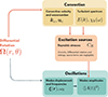 |
Fig. 2. Interdependencies in the stochastic excitation formalism with DR. The red arrows denote the direct impact of DR on convection we take into account, while the dotted arrows represent phenomena we do not take into account. The dark arrows represent the general interdependencies in the stochastic excitation formalism. |
2.3. Rotating convection
To model the local influence of DR on turbulent convection, we made use of the prescription from Augustson & Mathis (2019) of R-MLT. This formalism is a modified version of the mixing length theory (e.g. Böhm-Vitense 1958), and it takes into account the effects of the Coriolis acceleration. It is a single-mode approach that follows the heat flux maximisation principle proposed by Malkus (1954): The convective flow is dominated and modelled by the mode that transports the most amount of heat. R-MLT has been successfully compared with local direct numerical simulations in a Cartesian geometry (see e.g. Barker et al. 2014; Currie et al. 2020) as well as with global large eddy simulations for the prediction of the convective penetration (Korre & Featherstone 2021). It also has given some insightful results for the modelling of light elements mixing in low-mass stars (Dumont et al. 2021) and the thermal properties of the convective core boundary in early-type stars (Michielsen et al. 2019). Augustson & Mathis (2019) do not account for the term  in the momentum equation in their model (e.g. Unno et al. 1989). We thus considered convective length scales, which are much smaller than those associated with the latitudinal variation of the angular velocity. By doing so, we treat the impact of DR on convection locally.
The convective velocity (resp. convective wavenumber) with rotation, uc (resp. kc), is expressed as a function of the convective velocity (resp. convective wavenumber) without rotation, u0 (resp. k0):
 (18)
(18)
We introduced the Rossby number into the equation following Stevenson (1979), which represents the ratio between the advection and Coriolis acceleration:
 (19)
(19)
with θ being the co-latitude. In this definition, the Rossby number represents the ratio between the convective turnover frequency and the frequency associated with the vertical component of the rotation vector. Augustson & Mathis (2019) have shown that only the local vertical component of the rotation vector influences convection when assuming the principle of heat-flux maximisation, in which the heat is transported by the most unstable mode within R-MLT. Note that in other studies, such as Augustson & Mathis (2019), the Rossby number is defined without the explicit cos θ dependence. In these cases, the latitudinal variation of the rotation vector is instead incorporated directly into the governing equations.
In the formalism by Augustson & Mathis (2019), one can find the velocity modulation and the wavenumber modulation:
 (20)
(20)
 (21)
(21)
where z is the solution of the polynomial equation corresponding to Eq. (46) in Augustson & Mathis (2019):
 (22)
(22)
Here,  is a dimensionless prefactor defined as
  . (For more information, see Appendix A of Bessila et al. 2025, where we detail the R-MLT model from Augustson & Mathis 2019).
3. Impact of the differential rotation on the excitation of acoustic modes
3.1. Method
In this section, we compute the power injected by turbulent convection into the acoustic modes as a function of the DR. We follow the theoretical derivation expounded upon above. We used a solar-like 1 M⊙, Z = 0.02 1D model computed with the stellar evolution code MESA (Paxton et al. 2011, 2013, 2015, 2018, 2019; Jermyn et al. 2023) to evaluate convective non-rotating velocity and scale (u0, k0) and thermodynamical quantities (i.e. pressure and density). We used the stellar oscillation code GYRE (Townsend & Teitler 2013; Townsend et al. 2014) to compute stellar acoustic radial mode eigenfunctions, ξr; n, ℓ, m, and their eigenfrequencies.
For each mode, we used the following methodology:
-
We defined the DR rate, ΔΩ, and computed the resulting rotation profile.
-
For a given value of the local rotation, Ω, at a given radius and latitude, we computed the local effective Rossby number using the convective non-rotating properties u0 and k0 from MESA.
-
We then computed the convective velocity and convective wavenumber modified by rotation using Augustson & Mathis (2019) prescriptions for R-MLT (Equations 20 and 21).
-
Finally, we computed the resulting power injected into the modes by following the set of equations (14), (15) and (17).
In the following section, we take the mean rate of the Sun as a reference:  days (Thompson et al. 2012).
3.2. Results
We first examined the impact of DR on a fixed acoustic mode ℓ = 0, m = 0, n = 7. In our study of the uniform rotation (Bessila et al. 2025), we demonstrated that this mode’s amplitude is among the most significantly inhibited in rapidly rotating stars. Therefore, we focus on this mode in the present work. We used a 1 M⊙ solar-like model, with metallicity Z = 0.02 (see Appendix C for the MESA inlists). Here, we consider a fixed value for the turbulent spectrum slope: α = −5/3 (Kolmogorov 1941). For each value of the DR, we computed the power, 𝒫0, injected into the oscillations without rotation (Ω = 0) and the power, 𝒫Ω, injected taking DR into account.
Figure 3 shows the ratio 𝒫Ω/𝒫0 as a function of rotation for different values of the DR. Rotation tends to reduce the convection strength for the convective mode that transports the most amount of heat in the framework of R-MLT (Stevenson 1979; Augustson & Mathis 2019). In other words, the higher the rotation rate, the weaker the convective velocity with this model and the lower the power injected by the stochastic excitation. The impact of the DR on the Rossby number; convective velocity modulation,  ; and convective wavenumber modulation,
  , are shown in Fig. 4.
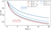 |
Fig. 3. Influence of the DR on the power injected in the acoustic mode (n = 7, ℓ = 0, m = 0) in a 1 M⊙, Z = 0.02 solar-like model. Anti-solar regimes, characterised by |


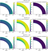 |
Fig. 4. Modification of the Rossby number (left panel), convective velocity (centre panel), and convective wavenumber (right panel) following Augustson & Mathis (2019) for a fixed mean rotation rate |


We note that for solar DR regimes (i.e. for ΔΩ > 0, in blue in Fig. 3), mode amplitudes are less influenced by the rotation, and hence they decrease less rapidly than in the case of uniform rotation when the rotation rate increases. The Rossby number as defined in Eq. (19) scales as ℛo ∼ 1/(Ω(θ)cos θ) and increases towards the equator. This means that rotation has less impact on convection near the equator than near the poles. For this reason, a rapidly rotating pole has more impact on convection than a slowly rotating pole. As a consequence, in the anti-solar DR regime (i.e. for ΔΩ < 0), where the poles rotate faster, mode amplitudes diminish more rapidly than in the uniform rotation case when rotation increases.
Secondly, there is an asymmetry in this result. For the same value of  , the difference in power injected between DR and uniform rotation is more pronounced in solar DR regimes than in anti-solar DR regimes. This is due to the local modification of the Rossby number: For a given value of the mean rotation rate,
  , at a fixed radius r and at the poles θ = 0, it scales as
 ![Mathematical equation: $ {\mathcal{R}\mathrm{o}} \sim u_0/[2\ell_0 \tilde{\Omega}(1+2A/3)] $](/articles/aa/full_html/2026/03/aa54366-25/aa54366-25-eq42.gif) . This function is not symmetric, and it increases more rapidly for A > 0 (i.e. solar DR regime) than for A < 0 (i.e. anti-solar DR regime). We illustrate this behaviour in Fig. 6. It then influences the convection in R-MLT differently and in turn the stochastic excitation of acoustic modes as well. Consequently, solar DR profiles exhibit a greater difference in the excitation power when compared to the uniform rotation case due to the more rapid variation in the Rossby number.
. This function is not symmetric, and it increases more rapidly for A > 0 (i.e. solar DR regime) than for A < 0 (i.e. anti-solar DR regime). We illustrate this behaviour in Fig. 6. It then influences the convection in R-MLT differently and in turn the stochastic excitation of acoustic modes as well. Consequently, solar DR profiles exhibit a greater difference in the excitation power when compared to the uniform rotation case due to the more rapid variation in the Rossby number.
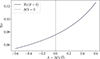 |
Fig. 6. Rossby number computed at the pole θ = 0 and at radius r = 0.8 R⊙ for |

Third, for a given |ΔΩ| value, the difference between solar and anti-solar DR rates increases with rotation rate. For a relative DR  , we find a difference of approximately 20% between the solar and anti-solar cases, for a 1Ω⊙ mean rotation rate.
Finally, Fig. 3 has to be considered with caution. Indeed, the relative DR is not a free parameter in our modelling, as it depends on the star’s age, mass, and its overall rotation rate (see e.g. Saar 2010; Brun et al. 2017, 2022). In particular, the anti-solar DR regime displayed in this figure is found in slowly rotating stars only, according to numerical simulations (see e.g. Noraz et al. 2022b).
As we have previously shown in Bessila et al. (2025), the power injected into the oscillations depends on the azimuthal order, m, due to the integral over the spherical harmonics in Eq. (14). Since the Rossby number is larger at the equator, the source term triggering the oscillations is weaker near the poles than at the equator. Axisymmetric modes, for which the spherical harmonics integral over the azimuth is maximum near the poles, thus exhibit lower amplitudes than their non-axisymmetric counterparts. We show in Fig. 5 the ℓ = 1, n = 7 mode amplitudes as a function of the mean rotation for different values of DR and for different azimuthal orders, m. As opposed to the trend for the m = 0 modes, the m = ±1 mode amplitudes are more inhibited in the solar DR regime. Indeed, the integral over the spherical harmonics in Eq. (14) gives more weight to the latitudes towards the equator than the polar region for this sectoral mode, as illustrated in Fig. 7. As the rotation rate at the equator is faster than the poles in the solar DR regime, the power injected into the m = 1 mode is more inhibited. Additionally, mode amplitudes vary significantly with azimuthal order. For example, for the ℓ = 1, n = 7 mode, amplitudes with m = ±1 are about 30% higher than the corresponding m = 0 mode amplitudes, for a 10Ω⊙ rotation rate. This is an interesting result, as it is often assumed in the literature that modes sharing the same radial order and spherical degree, ℓ, but differing in azimuthal order, m, carry the same energy. This hypothesis of equipartition is, for example, used to infer stellar inclinations from solar-like oscillations (Gizon & Solanki 2003). It would be interesting to extend such work to include the effects of the azimuthal order on the mode excitation. While the present paper focuses on the injection of energy in the modes, accounting for the effects of (differential) rotation on mode damping rates will also be essential to properly modelling mode amplitudes. Finally, better constraining the amplitudes of acoustic modes could provide valuable constrains on DR in solar-like stars. If this effect is detectable in observations, the amplitude ratio between axisymmetric and non-axisymmetric modes could serve as a proxy to constrain DR in solar-like stars. When a star’s average rotation rate is known, measuring the relative amplitudes of modes with the same ℓ and n but varying the m could provide insights into the rotational shear.
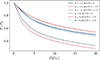 |
Fig. 5. Influence of the azimuthal order, m, on the power injected by the stochastic excitation for the ℓ = 1, n = 7 mode for different values of the DR. |
4. Dependance on the stellar mass and rotation
Differential rotation is not independent of the masses and rotation of the stars. Observational studies with Kepler have underlined that the DR tends to increase when stars rotate faster (Reinhold & Arlt 2015). It has been predicted that the DR scales similarly to a power law with the rotation  . The observational trends vary from r = 0.2 to r = 0.7, depending on the types of stars (Donahue et al. 1996; Reinhold & Reiners 2013; Balona & Abedigamba 2016). Through numerical simulations, the relationship between the DR and the rotation period has also been investigated (e.g. Brun et al. 2017, 2022). The exponent r was found to be r = 0.66 for hydrodynamical simulations (Brun et al. 2017), while it reduces to r = 0.46 in the framework of magnetohydrodynamical simulations (Brun et al. 2022). Another way to evaluate the DR is to assess the relative DR ΔΩ/Ω★. It depends on the star’s fluid Rossby number, which is defined as
 (23)
(23)
where  is the rms vorticity at the middle of the convective zone. The fluid Rossby number is a direct comparison of the convective advection term and the Coriolis acceleration in the Navier–Stokes equation. Saar (2010) and later Brun et al. (2022) both noticed that the relative DR is nearly constant for ℛof > 0.2, and it drops for fast rotators, ℛof ≤ 0.2, following
 (24)
(24)
The exponent was found to be p = 2 in the work by Saar (2010), while Brun et al. (2022) finds larger values: p ∈ [2, 6]. As mentioned in the introduction of this section, some transitions between different DR regimes have been found in numerical simulations (Gastine et al. 2013; Käpylä et al. 2014; Karak et al. 2015; Noraz et al. 2022a). For a fluid Rossby number above ℛof ∼ 1, stars exhibit an anti-solar DR profile.
In this section, we assess the impact of DR on the stochastic excitation of modes using Saar (2010), Brun et al. (2022) observations for the exponent p in Eq. (24). To this end, we first computed the stellar models with masses ranging from M = 0.8 M⊙ to M = 1.1 M⊙ and a Z = 0.02 metallicity at the mid-main sequence. Their path on the Hertzsprung-Russell diagram as well as their profiles for density, non-rotating convective velocity, and convective mixing length (the inverse of the non-rotating convective wavenumber k0 in our formalism) are detailed in Appendix A. Second, we computed their fluid Rossby number depending on their rotation rate. We used the scaling proposed by Noraz et al. (2022b) in their equation (18):
 (25)
(25)
where Teff, ⊙ and ℛof, ⊙ are the effective temperature and fluid Rossby number of the Sun, respectively. The solar fluid Rossby number is between 0.6 and 0.9 according to numerical simulations (e.g. Brun et al. 2022). The difference arises from the convective conundrum, which reflects uncertainties in our understanding of solar convection (Hanasoge et al. 2015; Noraz et al. 2025). In this work, we chose to take ℛof, ⊙ = 0.75 and Teff, ⊙ = 5772 K. We then assessed the relative DR rate of the stars following Eq. (24), with p ∈ [2, 6] as an exponent, which gives the lower and upper limits for the relative DR rate according to Brun et al. (2022). The results for the fluid Rossby number and the relative DR according to Eqs. (24) and (25) are plotted in Fig. 8. In agreement with other works such as Noraz et al. (2024), the relative DR is smaller for low-mass stars at a given mean rotation rate. This is due to the fluid Rossby number being smaller for smaller stellar masses. In addition, we took the relative DR as a constant for low rotation rates, i.e. for ℛof > 0.2, as highlighted by previous works (Saar 2010; Brun et al. 2022).
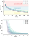 |
Fig. 8. Top: Fluid Rossby number according to Eq. (25) from Noraz et al. (2022b). Here, we specify the predicted DR regime. Bottom: Relative DR according to the scaling Eq. (24) from Brun et al. (2022). As the exponent p for these scaling laws is between p = 2 and 6, we represent for each model the range of possible values. The choice for the exponent p = 6 leads to a steeper diminution of the DR, when the overall rotation increases. |
Next, we computed the power injected in the oscillations using the stochastic excitation formalism. For values of fluid Rossby number greater than one (i.e. low-rotation rates), we assumed an anti-solar DR profile. We show the resulting power injected into the mode (ℓ = 0, m = 0, n = 7) while taking into account DR in Fig. 9. In the anti-solar case, the power injected into the modes diminishes more rapidly when rotation increases compared to the uniform rotation case. For a given stellar mass, when the rotation rate increases, the fluid Rossby number diminishes. When the fluid Rossby number goes below unity, around  , the rotation regime switches to a solar DR profile. From there, the power diminishes less when rotation increases compared to the uniform rotation case, in agreement with Fig. 3 where we highlight that a solar DR makes the modes less inhibited by rotation than in the uniformly rotating case. Acoustic modes in stars with anti-solar DR would then be more difficult to detect than stars in the uniformly rotating case. This must be taken into account when hunting stars hosting potentially anti-solar DR (Noraz et al. 2022b).
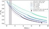 |
Fig. 9. Relative power injected into the oscillations with rotation compared to the non-rotating case for mode (ℓ = 0, n = 7, m = 0) using the scalings given in Eqs. (24) and (25). The dashed line represents the anti-solar DR regimes. As in Fig. 8, from |

Finally, we computed the power injected in the modes with the same angular degree, ℓ, but a different azimuthal number, m. We show the result in Fig. 10, for a 1 M⊙ stellar model. In this figure, all the modes are not equally influenced by rotation. For the sectoral modes with m = ±ℓ, taking solar DR into account results in more inhibited mode amplitudes in the solar DR regime, as opposed to what we witnessed for the other modes. As explained in Sect. 4, for the sectoral modes, the azimuthal integral of the spherical harmonics modulus in Eq. (14) gives more weight to equatorial amplitudes, resulting in less power injected into the acoustic modes than for the uniform rotation case (see Figs. 7 and 10). Moreover, we find the same trend for less massive solar-like stars (with M = 0.8 M⊙ and for more massive solar-like stars (with M = 1.2 M⊙), as shown in Appendix B in Figs. B.1 and B.2.
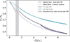 |
Fig. 10. Influence on the angular degree and azimuthal number on the power injected by the stochastic excitation. Top: ℓ = 1, n = 7 modes. Bottom: ℓ = 2, n = 7 modes. |
5. Conclusion and perspectives
In this work, we have studied for the first time the impact of DR on acoustic mode excitation by turbulent convection in pulsating main-sequence solar-like stars while taking into account a conical DR profile in their convective zone. We extended the theoretical formalism derived by Samadi & Goupil (2001), Belkacem et al. (2009) and Bessila et al. (2025), and we considered that turbulent convection is locally modified by DR. We modelled this modification using R-MLT (Stevenson 1979; Augustson & Mathis 2019), a single-mode approach of convection that predicts that rapid rotation modifies convection. According to this approach, the convective velocity and the characteristic turbulent eddy size become diminished when rotation increases.
In this framework, we find in general that the higher the rotation rate, the lower the mode amplitudes. More specifically, an anti-solar DR leads to a stronger diminution compared to the uniformly rotating case. Conversely, a solar DR profile leads to a slower diminution when the overall rotation rate increases compared to the uniform rotation case. We found asymmetry in this tendency. For the same value of |ΔΩ|, modes are more affected by rotation for a solar DR. Next, we applied these results to compute the power injected by the stochastic excitation for mid-main sequence solar-like stars with masses ranging from 0.8 to 1.1 M⊙. We used the scaling provided by Saar (2010), Brun et al. (2022), Noraz et al. (2022b) to model the variation of the DR with stellar mass and rotation based on state-of-the-art observations and large-eddy numerical simulations of the dynamics of differentially rotating convective envelopes of low-mass stars in spherical geometry, both in the hydrodynamical and magnetohydrodynamical cases. Such relations are suitable for qualitative estimates, although one must keep in mind that reality is more complex. We find that the power injected into the modes diminishes more slowly for values of Ω ≈ 1Ω⊙ when the stars are predicted to transition from an anti-solar to a solar DR profile. We also studied the influence of the azimuthal order m, which leads to a variation in the mode amplitudes, as highlighted before for the uniform rotation case (Bessila et al. 2025). It would be interesting to take this result into account when inferring stellar inclinations for observations and go beyond the equipartition hypothesis (Gizon & Solanki 2003). We have also shown that for the sectoral modes, with ℓ = ±m, the solar DR regime results in more inhibited amplitudes than for the uniform rotation case. These results highlight that the anti-solar rotation regime observed in numerical simulations might be more difficult to detect with asteroseismology, as acoustic modes are less excited when compared to the uniform rotation case at a fixed mean rotation. This outcome will be useful to predict the mode detection probability in the preparation of the PLATO mission (Rauer et al. 2014, 2025; Goupil et al. 2024). However, mode amplitudes involve a balance between driving and damping (see e.g. Samadi et al. 2015). To correctly assess the detection probability, one must also model the damping with DR. This is not investigated in the present paper and left for future work. Additionally, evaluating the impact of metallicity on the relative variation of DR (see e.g. See et al. 2021; Noraz et al. 2022b), and consequently on stochastic excitation, would provide further insights.
To go further, deriving a model with both the magnetic field and DR is crucial. Magnetic fields are ubiquitous in solar-like stars and are known to reduce the amplitudes of stochastically excited acoustic modes (Bessila & Mathis 2024), in agreement with observational trends reported by Garcia et al. (2010), Chaplin et al. (2011), and Mathur et al. (2019). In late-type stars, magnetic fields are generated through dynamo action within their convective envelopes. This process involves a complex interplay between latitudinal shear and the magnetic field, such as the Ω-effect, which is one of the key mechanisms driving this dynamo (Charbonneau 2014; Brun et al. 2022). Consequently, DR plays a critical role in our understanding of the generation of magnetic fields and the redistribution of angular momentum as a back reaction in the convective envelope of low-mass stars. For these reasons, our model of the stochastic excitation of acoustic modes must be extended to tackle the combined impact of DR and magnetic fields. This would allow for more accurate predictions of acoustic mode amplitudes within a more general and realistic framework.
Acknowledgments
L.B. and S.M. thank the referee for their comments that considerably improved the manuscript. L.B. and S.M. acknowledge support from the European Research Council (ERC) under the Horizon Europe programme (Synergy Grant agreement 101071505: 4D-STAR), from the CNES SOHO-GOLF and PLATO grants at CEA-DAp, and from PNPS (CNRS/INSU). While partially funded by the European Union, views and opinions expressed are, however, those of the authors only and do not necessarily reflect those of the European Union or the European Research Council. Neither the European Union nor the granting authority can be held responsible for them.
References
- Aerts, C., Christensen-Dalsgaard, J., & Kurtz, D. W. 2010, Asteroseismology (Springer Science+Business Media) [Google Scholar]
- Augustson, K. C., & Mathis, S. 2019, ApJ, 874, 83 [Google Scholar]
- Baglin, A., Auvergne, M., Boisnard, L., et al. 2006, 36th COSPAR Scientific Assembly, 36, 3749 [Google Scholar]
- Balmforth, N. J. 1992, MNRAS, 255, 639 [NASA ADS] [Google Scholar]
- Balona, L. A., & Abedigamba, O. P. 2016, MNRAS, 461, 497 [NASA ADS] [CrossRef] [Google Scholar]
- Barker, A. J., Dempsey, A. M., & Lithwick, Y. 2014, ApJ, 791, 13 [Google Scholar]
- Barnes, J. R., Cameron, A. C., Donati, J.-F., et al. 2005, MNRAS, 357, L1 [NASA ADS] [CrossRef] [Google Scholar]
- Bazot, M., Benomar, O., Christensen-Dalsgaard, J., et al. 2019, A&A, 623, A125 [NASA ADS] [CrossRef] [EDP Sciences] [Google Scholar]
- Belkacem, K. 2008, Theses, Observatoire de Paris [Google Scholar]
- Belkacem, K., Samadi, R., Goupil, M. J., & Dupret, M. A. 2008, A&A, 478, 163 [NASA ADS] [CrossRef] [EDP Sciences] [Google Scholar]
- Belkacem, K., Mathis, S., Goupil, M. J., & Samadi, R. 2009, A&A, 508, 345 [NASA ADS] [CrossRef] [EDP Sciences] [Google Scholar]
- Belkacem, K., Samadi, R., Goupil, M. J., et al. 2010, A&A, 522, L2 [NASA ADS] [CrossRef] [EDP Sciences] [Google Scholar]
- Benomar, O., Takata, M., Shibahashi, H., Ceillier, T., & García, R. A. 2015, MNRAS, 452, 2654 [Google Scholar]
- Benomar, O., Bazot, M., Nielsen, M. B., et al. 2018, Science, 361, 1231 [Google Scholar]
- Bessila, L., & Mathis, S. 2024, A&A, 690, A270 [NASA ADS] [CrossRef] [EDP Sciences] [Google Scholar]
- Bessila, L., Ruys, A. D. V., Buriasco, V., et al. 2025, A&A, 700, A25 [NASA ADS] [CrossRef] [EDP Sciences] [Google Scholar]
- Böhm-Vitense, E. 1958, Z. Astrophys., 46, 108 [Google Scholar]
- Borucki, W., Koch, D., Batalha, N., et al. 2008, Proc. Int. Astron. Union, 4, 289 [CrossRef] [Google Scholar]
- Borucki, W. J., Koch, D., Basri, G., et al. 2010, Science, 327, 977 [Google Scholar]
- Brun, A. S., & Browning, M. K. 2017, Liv. Rev. Sol. Phys., 14, 4 [Google Scholar]
- Brun, A. S., Strugarek, A., Varela, J., et al. 2017, ApJ, 836, 192 [Google Scholar]
- Brun, A. S., Strugarek, A., Noraz, Q., et al. 2022, ApJ, 926, 21 [NASA ADS] [CrossRef] [Google Scholar]
- Chaplin, W. J., Elsworth, Y., Isaak, G. R., Miller, B. A., & New, R. 1999, MNRAS, 308, 424 [Google Scholar]
- Chaplin, W. J., Houdek, G., Elsworth, Y., et al. 2005, MNRAS, 360, 859 [NASA ADS] [CrossRef] [Google Scholar]
- Chaplin, W. J., Appourchaux, T., Elsworth, Y., et al. 2010, ApJ, 713, L169 [NASA ADS] [CrossRef] [Google Scholar]
- Chaplin, W. J., Kjeldsen, H., Bedding, T. R., et al. 2011, ApJ, 732, 54 [CrossRef] [Google Scholar]
- Charbonneau, P. 2005, Dynamo Models of the Solar Cycle Living Reviews in Solar Physics, Tech. Rep. [Google Scholar]
- Charbonneau, P. 2014, ARA&A, 52, 251 [NASA ADS] [CrossRef] [Google Scholar]
- Christensen-Dalsgaard, J. 2021, Liv. Rev. Sol. Phys., 18, 2 [NASA ADS] [CrossRef] [Google Scholar]
- Couvidat, S., Garca, R. A., Turck-Chize, S., et al. 2003, ApJ, 597, L77 [Google Scholar]
- Currie, L. K., Barker, A. J., Lithwick, Y., & Browning, M. K. 2020, MNRAS, 493, 5233 [CrossRef] [Google Scholar]
- Deheuvels, S., Ballot, J., Beck, P. G., et al. 2015, A&A, 580, A96 [NASA ADS] [CrossRef] [EDP Sciences] [Google Scholar]
- Donahue, R. A., Saar, S. H., & Baliunas, S. L. 1996, ApJ, 466, 384 [Google Scholar]
- Donati, J.-F., & Cameron, A. C. 1997, MNRAS, 291, 1 [NASA ADS] [CrossRef] [Google Scholar]
- Dumont, T., Palacios, A., Charbonnel, C., et al. 2021, A&A, 646, A48 [EDP Sciences] [Google Scholar]
- Ecke, R. E., & Shishkina, O. 2023, Annu. Rev. Fluid Mech., 55, 603 [Google Scholar]
- Eff-Darwich, A., & Korzennik, S. G. 2013, Sol. Phys., 287, 43 [NASA ADS] [CrossRef] [Google Scholar]
- García, R. A., & Ballot, J. 2019, Liv. Rev. Sol. Phys., 16, 4 [Google Scholar]
- García, R. A., Turck-Chièze, S., Jiménez-Reyes, S. J., et al. 2007, Science, 316, 1591 [Google Scholar]
- Garcia, R. A., Mathur, S., Salabert, D., et al. 2010, Science, 329, 1032 [NASA ADS] [CrossRef] [Google Scholar]
- Gastine, T., Yadav, R. K., Morin, J., Reiners, A., & Wicht, J. 2013, MNRAS, 438, L76 [NASA ADS] [CrossRef] [Google Scholar]
- Gilman, P. A. 1977, Geophys. Astrophys. Fluid Dyn., 8, 93 [NASA ADS] [CrossRef] [Google Scholar]
- Gilman, P. A., & Glatzmaier, G. A. 1981, ApJS, 45, 335 [CrossRef] [Google Scholar]
- Gizon, L., & Solanki, S. K. 2003, ApJ, 589, 1009 [Google Scholar]
- Goldreich, P., & Keeley, D. A. 1977, ApJ, 212, 243 [NASA ADS] [CrossRef] [Google Scholar]
- Goupil, M. J., Catala, C., Samadi, R., et al. 2024, A&A, 683, A78 [NASA ADS] [CrossRef] [EDP Sciences] [Google Scholar]
- Grigahcène, A., Dupret, M.-A., Gabriel, M., Garrido, R., & Scuflaire, R. 2005, A&A, 434, 1055 [NASA ADS] [CrossRef] [EDP Sciences] [Google Scholar]
- Guerrero, G., Smolarkiewicz, P. K., Kosovichev, A. G., & Mansour, N. N. 2013, ApJ, 779, 176 [NASA ADS] [CrossRef] [Google Scholar]
- Hanasoge, S., Miesch, M. S., Roth, M., et al. 2015, Space Sci. Rev., 196, 79 [NASA ADS] [CrossRef] [Google Scholar]
- Howell, S. B., Sobeck, C., Haas, M., et al. 2014, PASP, 126, 398 [Google Scholar]
- Huber, D., Chaplin, W. J., Chontos, A., et al. 2019, AJ, 157, 245 [Google Scholar]
- Jermyn, A. S., Bauer, E. B., Schwab, J., et al. 2023, ApJS, 265, 15 [NASA ADS] [CrossRef] [Google Scholar]
- Jouve, L., Brown, B. P., & Brun, A. S. 2010, A&A, 509, 1 [Google Scholar]
- Käpylä, P. J., Käpylä, M. J., & Brandenburg, A. 2014, A&A, 570, A43 [NASA ADS] [CrossRef] [EDP Sciences] [Google Scholar]
- Karak, B. B., Käpylä, P. J., Käpylä, M. J., et al. 2015, A&A, 576, A26 [NASA ADS] [CrossRef] [EDP Sciences] [Google Scholar]
- Kolmogorov, A. N. 1941, Doklady Akad. Nauk. SSR, 434 [Google Scholar]
- Korre, L., & Featherstone, N. A. 2021, ApJ, 923, 52 [NASA ADS] [CrossRef] [Google Scholar]
- Kovári, Z., Bartus, J., Švanda, M., et al. 2007, Astron. Nachr., 328, 1081 [CrossRef] [Google Scholar]
- Malkus, W. V. R. 1954, Proc. R. Soc. London Ser. A, 225, 196 [Google Scholar]
- Mathur, S., Garcia, R. A., Bugnet, L., et al. 2019, Front. Astron. Space Sci., 6, 46 [Google Scholar]
- Matt, S. P., Do Cao, O., Brown, B. P., & Brun, A. S. 2011, Astron. Nachr., 332, 897 [NASA ADS] [CrossRef] [Google Scholar]
- Michel, E., Baglin, A., Auvergne, M., et al. 2008, Science, 322, 558 [Google Scholar]
- Michielsen, M., Pedersen, M. G., Augustson, K. C., Mathis, S., & Aerts, C. 2019, A&A, 628, A76 [NASA ADS] [CrossRef] [EDP Sciences] [Google Scholar]
- Neiner, C., Lee, U., Mathis, S., et al. 2020, A&A, 644, A9 [EDP Sciences] [Google Scholar]
- Noraz, Q., Brun, A. S., Strugarek, A., & Depambour, G. 2022a, A&A, 658, A144 [NASA ADS] [CrossRef] [EDP Sciences] [Google Scholar]
- Noraz, Q., Breton, S. N., Brun, A. S., et al. 2022b, A&A, 667, A50 [NASA ADS] [CrossRef] [EDP Sciences] [Google Scholar]
- Noraz, Q., Brun, A. S., & Strugarek, A. 2024, arXiv e-prints [arXiv:2401.14460] [Google Scholar]
- Noraz, Q., Brun, A. S., Strugarek, A., et al. 2025, arXiv e-prints [arXiv:2501.13169] [Google Scholar]
- Oláh, K., Kolláth, Z., Granzer, T., et al. 2009, A&A, 501, 703 [NASA ADS] [CrossRef] [EDP Sciences] [Google Scholar]
- Paxton, B., Bildsten, L., Dotter, A., et al. 2011, ApJS, 192, 3 [Google Scholar]
- Paxton, B., Cantiello, M., Arras, P., et al. 2013, ApJS, 208, 4 [Google Scholar]
- Paxton, B., Marchant, P., Schwab, J., et al. 2015, ApJS, 220, 15 [Google Scholar]
- Paxton, B., Schwab, J., Bauer, E. B., et al. 2018, ApJS, 234, 34 [NASA ADS] [CrossRef] [Google Scholar]
- Paxton, B., Smolec, R., Schwab, J., et al. 2019, ApJS, 243, 10 [Google Scholar]
- Proudman, J. 1916, Proc. Roy. Soc. London Ser. A, 92, 408 [Google Scholar]
- Rauer, H., Catala, C., Aerts, C., et al. 2014, Exp. Astron., 38, 249 [Google Scholar]
- Rauer, H., Aerts, C., Cabrera, J., et al. 2025, Exp. Astron., 59, 26 [Google Scholar]
- Reinhold, T., & Arlt, R. 2015, A&A, 576, A15 [NASA ADS] [CrossRef] [EDP Sciences] [Google Scholar]
- Reinhold, T., & Reiners, A. 2013, A&A, 557, A11 [NASA ADS] [CrossRef] [EDP Sciences] [Google Scholar]
- Ricker, G. R., Winn, J. N., Vanderspek, R., et al. 2014, Proc. SPIE, 9143, 914320 [Google Scholar]
- Saar, S. H. 2010, Proc. Int. Astron. Union, 6, 61 [Google Scholar]
- Saar, S. H., & Brandenburg, A. 1999, ApJ, 524, 295 [NASA ADS] [CrossRef] [Google Scholar]
- Samadi, R., & Goupil, M.-J. 2001, A&A, 370, 136 [NASA ADS] [CrossRef] [EDP Sciences] [Google Scholar]
- Samadi, R., Goupil, M. J., Alecian, E., et al. 2005, JApA, 26, 171 [NASA ADS] [Google Scholar]
- Samadi, R., Georgobiani, D., Trampedach, R., et al. 2007, A&A, 463, 297 [NASA ADS] [CrossRef] [EDP Sciences] [Google Scholar]
- Samadi, R., Belkacem, K., & Sonoi, T. 2015, EAS Publ. Ser., 73–74, 111 [Google Scholar]
- Schou, J., Antia, H. M., Basu, S., et al. 1998, ApJ, 505, 390 [Google Scholar]
- See, V., Roquette, J., Amard, L., & Matt, S. P. 2021, ApJ, 912, 127 [Google Scholar]
- Stein, R. F. 1967, Sol. Phys., 2, 385 [NASA ADS] [CrossRef] [Google Scholar]
- Stevenson, D. J. 1979, Geophys. Astrophys. Fluid Dyn., 12, 139 [NASA ADS] [CrossRef] [Google Scholar]
- Taylor, G. I. 1917, Proc. Roy. Soc. London Ser. A, 93, 99 [Google Scholar]
- Thompson, M. J., Christensen-Dalsgaard, J., Miesch, M. S., & Toomre, J. 2003, ARA&A, 41, 599 [Google Scholar]
- Thompson, S. E., Everett, M., Mullally, F., et al. 2012, ApJ, 753, 86 [Google Scholar]
- Townsend, R. H. D., & Teitler, S. A. 2013, MNRAS, 435, 3406 [Google Scholar]
- Townsend, R., Teitler, S., & Paxton, B. 2014, Proc. Int. Astron. Union, 301, 505 [Google Scholar]
- Unno, W., Osaki, Y., & Ando, H. 1989, Non-radial Oscillations of Stars, 2nd edn. (Tokyo: University of Tokyo Press) [Google Scholar]
Appendix A: Properties of the computed stellar models
We detail in this section the properties of the stellar models used in Sec. 4. The radial profiles of the density and the non-rotating convective characteristic mixing-length and velocity are displayed in Fig. A.1. The corresponding Hertzsprung-Russell diagrams are plotted in Fig. A.2. We study models with different stellar masses from 0.8 M⊙ to 1.1 M⊙, at a metallicity Z = 0.02, at mid-main sequence.
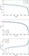 |
Fig. A.1. Density profile, ρ0 (top), and non-rotating convective characteristic mixing-length, ℓ0 (middle), and velocity, u0 (bottom). Note that the radius, r, is normalised to each stellar radius, R★. |
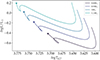 |
Fig. A.2. Position of the different stellar models in the Hertzsprung-Russell diagram. |
Appendix B: Influence of the azimuthal number for different stellar models
In this section, we compute the power injected by the stochastic excitation for stellar models with M = 0.8 M⊙ and M = 1.1 M⊙. We retrieve the same trend as in Fig. 9: in the models with a higher mass, the modes are less inhibited by the rotation.
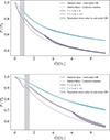 |
Fig. B.1. Influence of the DR on the stochastic excitation of the modes ℓ = 1, n = 7 and different values of m. (Top) 0.8 M⊙ model (Bottom) 1.1 M⊙ model. |
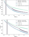 |
Fig. B.2. Influence of the DR on the stochastic excitation of the modes ℓ = 2, n = 7 and different values of m. (Top) 0.8 M⊙ model (Bottom) 1.1 M⊙ model. |
Appendix C: MESA inlists for the solar model
&kap
  ! kap options
  ! see kap/defaults/kap.defaults
  use_Type2_opacities = .true.
    Zbase = 0.016

/ ! end of kap namelist

&controls
      initial_mass = 1.0

      ! MAIN PARAMS
      mixing_length_alpha = 1.9446893445
      initial_z = 0.02 ! 0.04, 0.002, 0.026
      do_conv_premix = .true.
      use_Ledoux_criterion = .true.

      ! OUTPUT
      max_num_profile_models = 100000
      profile_interval = 300
      history_interval = 1
      photo_interval = 300

      ! WHEN TO STOP
      xa_central_lower_limit_species(1) = 'h1'
      xa_central_lower_limit(1) = 0.01
      max_age = 6.408d9

      ! RESOLUTION
      mesh_delta_coeff = 0.5
      time_delta_coeff = 1.0

      ! GOLD TOLERANCES
      use_gold_tolerances = .true.
      use_gold2_tolerances = .true.
      delta_lg_XH_cntr_limit = 0.01
      min_timestep_limit = 1d-1

      !limit on magnitude
      delta_lgTeff_limit = 0.25 ! 0.005
      delta_lgTeff_hard_limit = 0.25 ! 0.005
      delta_lgL_limit = 0.25 ! 0.005

      ! asteroseismology
      write_pulse_data_with_profile = .true.
      pulse_data_format = 'FGONG'
      ! add_atmosphere_to_pulse_data = .true.


/ ! end of controls namelist


&pgstar


/ ! end of pgstar namelist
All Figures
|
Fig. 1. Conical DR profile for a solar regime (top) and an anti-solar regime (bottom) following Eq. (1). In both cases, |
| In the text | |
|
Fig. 2. Interdependencies in the stochastic excitation formalism with DR. The red arrows denote the direct impact of DR on convection we take into account, while the dotted arrows represent phenomena we do not take into account. The dark arrows represent the general interdependencies in the stochastic excitation formalism. |
| In the text | |
|
Fig. 3. Influence of the DR on the power injected in the acoustic mode (n = 7, ℓ = 0, m = 0) in a 1 M⊙, Z = 0.02 solar-like model. Anti-solar regimes, characterised by |
| In the text | |
|
Fig. 4. Modification of the Rossby number (left panel), convective velocity (centre panel), and convective wavenumber (right panel) following Augustson & Mathis (2019) for a fixed mean rotation rate |
| In the text | |
|
Fig. 6. Rossby number computed at the pole θ = 0 and at radius r = 0.8 R⊙ for |
| In the text | |
|
Fig. 5. Influence of the azimuthal order, m, on the power injected by the stochastic excitation for the ℓ = 1, n = 7 mode for different values of the DR. |
| In the text | |
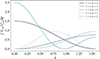 |
Fig. 7. Azimuthal integral of the modulus of the spherical harmonics |
| In the text | |
|
Fig. 8. Top: Fluid Rossby number according to Eq. (25) from Noraz et al. (2022b). Here, we specify the predicted DR regime. Bottom: Relative DR according to the scaling Eq. (24) from Brun et al. (2022). As the exponent p for these scaling laws is between p = 2 and 6, we represent for each model the range of possible values. The choice for the exponent p = 6 leads to a steeper diminution of the DR, when the overall rotation increases. |
| In the text | |
|
Fig. 9. Relative power injected into the oscillations with rotation compared to the non-rotating case for mode (ℓ = 0, n = 7, m = 0) using the scalings given in Eqs. (24) and (25). The dashed line represents the anti-solar DR regimes. As in Fig. 8, from |
| In the text | |
|
Fig. 10. Influence on the angular degree and azimuthal number on the power injected by the stochastic excitation. Top: ℓ = 1, n = 7 modes. Bottom: ℓ = 2, n = 7 modes. |
| In the text | |
|
Fig. A.1. Density profile, ρ0 (top), and non-rotating convective characteristic mixing-length, ℓ0 (middle), and velocity, u0 (bottom). Note that the radius, r, is normalised to each stellar radius, R★. |
| In the text | |
|
Fig. A.2. Position of the different stellar models in the Hertzsprung-Russell diagram. |
| In the text | |
|
Fig. B.1. Influence of the DR on the stochastic excitation of the modes ℓ = 1, n = 7 and different values of m. (Top) 0.8 M⊙ model (Bottom) 1.1 M⊙ model. |
| In the text | |
|
Fig. B.2. Influence of the DR on the stochastic excitation of the modes ℓ = 2, n = 7 and different values of m. (Top) 0.8 M⊙ model (Bottom) 1.1 M⊙ model. |
| In the text | |
Current usage metrics show cumulative count of Article Views (full-text article views including HTML views, PDF and ePub downloads, according to the available data) and Abstracts Views on Vision4Press platform.
Data correspond to usage on the plateform after 2015. The current usage metrics is available 48-96 hours after online publication and is updated daily on week days.
Initial download of the metrics may take a while.