| Issue |
A&A
Volume 707, March 2026
|
|
|---|---|---|
| Article Number | A387 | |
| Number of page(s) | 19 | |
| Section | Astronomical instrumentation | |
| DOI | https://doi.org/10.1051/0004-6361/202554409 | |
| Published online | 25 March 2026 | |
Mutual impedance experiments in a laboratory plasma
Experimental validation of numerical modeling
1
Laboratoire de Physique et Chimie de l’Environnement et de l’Espace (LPC2E), CNRS, Université d’Orléans,
Orléans,
France
2
LESIA, Observatoire de Paris, PSL Research University, CNRS, Sorbonne Université, UPMC, Université Paris Diderot, Sorbonne Paris Cité,
Meudon,
France
3
Laboratoire Lagrange, OCA, UCA, CNRS,
Nice,
France
4
LPP, Sorbonne Université, CNRS, Ecole Polytechnique,
91128
Palaiseau,
France
5
Space Physics Division, Royal Belgian Institute for Space Aeronomy (BIRA-IASB),
Ringlaan 3,
1180
Brussels,
Belgium
6
Center for mathematical Plasma Astrophysics, Katholieke Universiteit Leuven,
Celestijnenlaan 200B,
3001
Heverlee,
Belgium
7
Swedish Institute of Space Physics (IRF),
Uppsala,
Sweden
8
Laboratoire Plasma et Conversion d’Energie (LAPLACE), Université de Toulouse, CNRS,
31062
Toulouse,
France
★ Corresponding author: This email address is being protected from spambots. You need JavaScript enabled to view it.
Received:
7
March
2025
Accepted:
30
January
2026
Abstract
Context. In situ measurements of space plasma are necessary to explore heliospheric and planetary ionized environments. Mutual impedance experiments are an active plasma diagnostic technique used to measure the properties of space plasmas, including the plasma density and the electron temperature. Although various models have been developed for unmagnetized space plasmas, they fail to describe the instrument behavior in magnetized plasmas, such as the ionosphere and magnetosphere of magnetized planets and moons. A quantitative instrument model of the mutual impedance experiment is required, however, for current and future space missions, including ESA/JAXA BepiColombo and ESA JUICE, which will both conduct mutual impedance experiments (PWI/AM2P and RPWI/MIME, respectively).
Aims. We develop an instrument model for exploring and quantitatively characterizing mutual impedance experiment measurements performed in planetary plasmas, with the goal of providing in situ diagnostics of the plasma density and electron temperature.
Methods. To reach this goal, we combined numerical investigation and laboratory experiments. We investigated the experimental regime of high magnetization for the first time, where the electron gyrofrequency is higher than the plasma frequency, both experimentally and numerically. On the experimental side, we built a setup composed of a plasma chamber, a mutual impedance experiment, and a Langmuir probe. With this, we achieved a controlled plasma environment representative of magnetized space plasmas, which we diagnosed with two independent plasma instruments. On the numerical side, we developed a model for magnetized mutual impedance experiments that took the geometry of the mutual impedance antennas and the plasma chamber into account and that employed a kinetic linear description of the plasma electrons.
Results. First, we characterized the plasma environment generated in the plasma chamber: the achievable plasma parameters, the stability, and the repeatability of the plasma conditions. Second, we validated the instrument model by comparing the numerical model predictions to the measurements obtained in the plasma chamber. Third, we extracted the plasma density and temperature from in situ mutual impedance measurements using our new numerical instrument model, and we validated them using the independent in situ measurements from the Langmuir probe.
Conclusions. This work (i) proves that mutual impedance experiments are able to provide robust plasma diagnostics in a magnetized space plasma environment, and (ii) develops a methodological framework that will be used for the planetary space missions BepiColombo and JUICE to perform both the in-flight calibration and the exploitation of the measurements from PWI/AM2P and RPWI/MIME, respectively, in the magnetospheres of Mercury, Jupiter, and Ganymede.
Key words: instrumentation: miscellaneous / methods: data analysis / planets and satellites: magnetic fields
© The Authors 2026
 Open Access article, published by EDP Sciences, under the terms of the Creative Commons Attribution License (https://creativecommons.org/licenses/by/4.0), which permits unrestricted use, distribution, and reproduction in any medium, provided the original work is properly cited.
This article is published in open access under the Subscribe to Open model. This email address is being protected from spambots. You need JavaScript enabled to view it. to support open access publication.
1 Introduction
Mutual impedance experiments are an in situ space plasma diagnostic technique that is used in particular for measuring the properties of the plasma electrons, including their density and temperature. These experiments measure the mutual impedance between a pair of electric antennas that are embedded in the plasma. The measurement is carried out by generating an electric perturbation inside the plasma with one antenna (defined as the emitting antenna) while simultaneously measuring the plasma response with the other antenna (defined as the receiving antenna). A detailed definition of the measurement procedure is provided in this paper. The quantity that is examined in mutual impedance experiments is the frequency spectrum of the plasma response. The underlying physics is the propagation of waves inside the plasma.
Different previous space missions have employed mutual impedance experiments in order to study a variety of plasma environments. Among them are the Earth’s ionosphere, for example with the FR-1 (Storey et al. 1969), DRAGON-3 (Beghin 1971), CISASPE (Chasseriaux et al. 1972), and PORCUPINE (Haeusler et al. 1979) missions, and magnetosphere, for example with the GEOS-1 (Decreau et al. 1978), ARCAD-3 (Béghin et al. 1982), and Viking (Perraut et al. 1990; Bahnsen et al. 1988) missions, as well as the atmosphere of Titan (Huygens probe (Hamelin et al. 2007)) and the plasma environment of comet 67P/Churyumov-Gerasimenko with the Rosetta plasma consortium mutual impedance probe (RPC/MIP) (Trotignon et al. 2007). Current planetary space missions also count mutual impedance experiments in their scientific payload, notably the active measurement of Mercury’s plasma experiment (AM2P) of the plasma wave investigation (PWI) (Kasaba et al. 2020; Karlsson et al. 2020) consortium onboard the ESA/JAXA BepiColombo mission (Benkhoff et al. 2010), the mutual impedance measurements (MIME) experiment of the radio wave plasma investigation (RPWI) (Wahlund et al. 2025) consortium onboard the ESA Jupiter ici moons explorer (JUICE) mission (Grasset et al. 2013), and the dust field plasma (DFP) cometary light plasma instrument (COMPLIMENT) (Snodgrass & Jones 2019) onboard the ESA Comet Interceptor mission (Snodgrass & Jones 2019).
When a mutual impedance experiment is used, a key step is obtaining a set of physically meaningful plasma parameters (e.g., the electron density and temperature) from the calibrated measurements, namely the mutual impedance spectrum. Different approaches can be employed, but nearly all of them require the use of an instrument model to interpret the measurements. One way to analyze these measurements is to find a best fit between the instrument model and the measurements as a function of the plasma parameters. Such an instrument model strongly benefits from being validated with measurements obtained in a controlled plasma environment. A laboratory plasma chamber, where a controlled plasma is produced, is therefore able to support the instrumental development. This was one of the reasons for the development of the testing facility Plasma Environment Platform for Satellite tests in Orléans (PEPSO) at the LPC2E (CNRS, Orléans, France) space laboratory. This plasma chamber has already been used to explore new instrumental modes for mutual impedance experiments by Bucciantini et al. (2023).
The instrument models used for the analysis of mutual impedance experiments have been developed with a particular focus on the limit of an unmagnetized plasma. This means that the effects of the magnetic field on the plasma diagnostic are not taken into account. This approximation is valid when the plasma frequency fpe is much higher than the electron cyclotron frequency fce: fpe/fce ≫ 1, with ![Mathematical equation: $\[f_{p e}=\frac{1}{2 \pi} \sqrt{\frac{n_{e} e^{2}}{m_{e} \varepsilon_{0}}}\]$](/articles/aa/full_html/2026/03/aa54409-25/aa54409-25-eq1.png) and
and ![Mathematical equation: $\[f_{c e}=\frac{1}{2 \pi} \frac{e B}{m_{e}}\]$](/articles/aa/full_html/2026/03/aa54409-25/aa54409-25-eq2.png) , where e and me are the electron charge and mass, respectively, B is the magnetic field strength, and ε0 is the vacuum electric permittivity. A new mutual impedance instrument model that extends to magnetized plasma has recently been developed (Dazzi et al. 2025). However, it is still lacking an experimental validation provided by the comparison of the modeling expectations to actual measurements. This validation step is necessary in order to prove the applicability of the new magnetized mutual impedance model to the PWI/AM2P and RPWI/MIME experiments.
, where e and me are the electron charge and mass, respectively, B is the magnetic field strength, and ε0 is the vacuum electric permittivity. A new mutual impedance instrument model that extends to magnetized plasma has recently been developed (Dazzi et al. 2025). However, it is still lacking an experimental validation provided by the comparison of the modeling expectations to actual measurements. This validation step is necessary in order to prove the applicability of the new magnetized mutual impedance model to the PWI/AM2P and RPWI/MIME experiments.
In this context, we here first validate the modeling of mutual impedance experiments in a magnetized plasma using laboratory measurements, and we then prove experimentally that it is possible to retrieve the plasma density and electron temperature in a magnetized plasma from mutual impedance experiments. We remark that in the context of mutual impedance experiments, we use the term magnetized plasma to indicate a plasma in which the ratio of plasma to electron cyclotron frequency is low (i.e., approximately fpe/fce ≲ 10); in this regime, the magnetic field affects the measurements significantly.
This paper is organized as follows. In Sect. 2 we introduce the model and the experimental setup. In Sect. 3 we describe the measurement sets we used. In Sect. 4 we detail the analysis technique used to interpret these measurements, in particular, the comparison between the measurements and the mutual impedance model, as well as the plasma parameters obtained from the mutual impedance experiment. We summarize our conclusions in Sect. 5.
2 Theoretical and experimental methods for mutual impedance experiments
In this section, we define the experimental setup and numerical modelling used to interpret mutual impedance experiments. The section is organized as follows: we define mutual impedance experiments (Sect. 2.1), we present the mutual impedance setup inside the plasma chamber (Sect. 2.2), and we describe the numerical mutual impedance instrument model (Sect. 2.3).
2.1 Definition of a mutual impedance experiment
In the following, we define the mutual impedance spectrum and describe the experimental procedure we used to perform mutual impedance measurements. These considerations also lead to the requirements for the model that is used to interpret these measurements.
As described in Sect. 1, the mutual impedance is defined for a set of two electrical antennas, embedded in a plasma. A schematic view of this antenna configuration is presented in the left panel of Fig. 1. An alternating current I(f) at a fixed frequency f is imposed between the electrodes of one of the antennas (defined as the emitting antenna). Simultaneously, the electric potential difference V(f) between the electrodes of the other antenna (defined as the receiving antenna) is measured. The ratio of the potential to the current is defined as the mutual impedance Z(f) = V(f)/I(f) between the two antennas. The mutual impedance spectrum is therefore defined as in standard antenna theory (Kraus 1997). In the context of plasma diagnostics, the mutual impedance Z is often normalized to its value obtained in vacuum Z0 to isolate the plasma contribution itself. Therefore, the quantity that is analyzed is Z/Z0.
A first possible experimental setup measuring the mutual impedance is made of a current generator connected to the emitting antenna and a voltmeter connected to the receiving antenna. The current generator, considered as ideal, delivers a constant current whatever the plasma conditions around the antenna and the chosen frequency. In this case, the normalized mutual impedance is Z/Z0 = V/V0, where V (respectively V0) is the electric potential measured in the presence (absence) of a plasma.
A second possible experimental setup instead relies on an ideal voltage generator delivering an alternating voltage difference of fixed amplitude between the electrodes of the emitting antenna. The fixed voltage amplitude is achieved by imposing a low-output impedance at the connection to the emitting antenna electrodes. With this experimental setup, the current at the emitting antenna is frequency dependent on a plasma. The measured quantity to be analyzed is V/V0, the ratio of voltages at the receiving antenna in the presence or absence of a plasma. As a consequence, V/V0 ≠ Z/Z0 when a voltage generator is used. In this case, the quantity V/V0 is used instead of the normalized mutual impedance Z/Z0. An instrument model that is used to interpret mutual impedance measurements obtained using a voltage generator therefore needs to be able to quantify the current flowing into the plasma from the emitting antenna. It must also take the voltage on the emitting antenna as input.
In order to reconstruct the mutual impedance spectrum, measurements of V/V0 are repeated by changing the frequency of emission f. We show an illustrative example of the potential imposed on the emitting antenna and of the potential measured at the receiving antenna in the upper middle panel of Fig. 1. For illustration purposes, we only show the first 4 μs of the signals at five selected frequencies. The potential difference measured simultaneously between the electrodes of the receiving antenna is shown in the lower middle panel of the same Fig. 1. The mutual impedance spectrum reconstructed from these measurements is shown in the right panel of Fig. 1 for the selected five frequencies in color and for the full spectrum in gray. This measurement procedure is referred to as a frequency sweep, and we used this to obtain the measurements described in this paper. We wish to highlight that it is not the only procedure that has been investigated (Bucciantini et al. 2023).
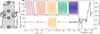 |
Fig. 1 Left: schematic view of a mutual impedance emitting and receiving antenna. Middle: emission and reception signals measured by a typical mutual impedance experiment for five selected frequencies (in different colors). Right: mutual impedance measured for these five frequencies using the same colors, together with the mutual impedance spectrum measured for many frequencies in gray. |
2.2 Experimental setup: PEPSO plasma chamber
In this section, we describe in detail the experimental setup. This section is organized as follows: we describe how the plasma chamber works (Sect. 2.2.1), the properties of the plasma that it produces (Sect. 2.2.2 and Sect. 2.2.3), and we finish by describing the plasma diagnostics present inside (Sect. 2.2.4).
2.2.1 Functioning principles of the PEPSO plasma chamber
The vacuum chamber is cylindrical and measures 1 m in diameter and 1.8 m in length. It is made of a AISI 304L stainless-steel alloy. This alloy is essentially nonmagnetic.
The pumping system is composed of two pumps acting in series: a primary multistage roots pump (Pfeiffer/ACP 40), and a secondary turbomolecular pump (Pfeiffer/ATH 3204 M). Together, they can reach a final pressure as low as 5 · 10−7 mbar measured at the bottom of the plasma chamber, close to the vacuum pump inlet.
The plasma source was based on the design of a Kaufman ion source for sputtering applications (Kaufman et al. 1982). It is used to produce a plasma starting from a neutral gas.
The employed gas was argon >99.999% pure, which has an ionization energy of around 15.8 eV. The argon gas was first injected in the ionization chamber. The ionization chamber was separated from the vacuum chamber and smaller.
An ionization filament, made of 0.25 mm diameter tungsten and around 80 mm long, was present inside the ionization chamber. This ionization filament was heated to a temperature Ti by passing a current inside it, named the ionization current Ii, and therefore, it emitted electrons by thermionic emission. The current density of emitted electrons J(i) is approximately described by Richardson’s law
![Mathematical equation: $\[J_{(i)} \propto T_{i}^{2} e^{-W /\left(k_{B} T_{i}\right)}\]$](/articles/aa/full_html/2026/03/aa54409-25/aa54409-25-eq3.png) , where W is the tungsten work function of around 5 eV (Grosso & Pastori Parravicini 2014). These electrons collide onto the neutral argon gas, ionizing part of it. An external solenoid surrounding the ionization chamber can be used to increase the electron path inside the ionization chamber, due to the electron gyration. This increases the probability to ionize argon by electron ionization and therefore increases the rate of plasma generation. This capability was only used to reach high plasma densities in the chamber.
, where W is the tungsten work function of around 5 eV (Grosso & Pastori Parravicini 2014). These electrons collide onto the neutral argon gas, ionizing part of it. An external solenoid surrounding the ionization chamber can be used to increase the electron path inside the ionization chamber, due to the electron gyration. This increases the probability to ionize argon by electron ionization and therefore increases the rate of plasma generation. This capability was only used to reach high plasma densities in the chamber.The produced positive Ar+ ions escape from the ionizing chamber, while the electrons remain inside thanks to the filtering grid that was kept at a fixed negative potential.
The last step consisted of neutralizing the positive argon ions escaping from the ionization chamber. This was done by heating the neutralizing filament by passing a current In through it. This filament was located just outside the filtering grid and also produced electrons by thermionic emission. These electrons neutralized the ion flow, so that a quasi-neutral plasma drifted inside the plasma chamber.
The typical values for the plasma density and electron temperature inside PEPSO, measured by the Langmuir probe are shown in Fig. 2, together with the associated values of the plasma frequency fpe and the Debye length ![Mathematical equation: $\[\lambda_{D e}=\sqrt{\frac{\varepsilon_{0} k_{B} T_{e}}{n_{e} e^{2}}}\]$](/articles/aa/full_html/2026/03/aa54409-25/aa54409-25-eq4.png) , where kB is Boltzmann’s constant. We worked under the assumption that the parallel and perpendicular electron temperature are equal. The argon gas injected in the plasma source was not completely ionized, so that some neutral argon flowed inside the plasma chamber. The electron-neutral argon mean-free-path was estimated to be about 100 m (Bucciantini et al. 2023; Gargioni & Grosswendt 2008), so that the plasma was considered to be collisionless.
, where kB is Boltzmann’s constant. We worked under the assumption that the parallel and perpendicular electron temperature are equal. The argon gas injected in the plasma source was not completely ionized, so that some neutral argon flowed inside the plasma chamber. The electron-neutral argon mean-free-path was estimated to be about 100 m (Bucciantini et al. 2023; Gargioni & Grosswendt 2008), so that the plasma was considered to be collisionless.
The magnetized mutual impedance model was tested in different plasma conditions by varying the plasma density inside the plasma chamber. The current imposed on the ionization filament Ii controls the flux of emitted electrons. These in turn ionize the Argon gas. The ionization current therefore controls the plasma density. Figure 3 shows the experimental relation between Ii and the plasma density and electron temperature, measured by a Langmuir probe. These measurements were obtained by using a fixed argon gas flow of 3 SCCM (standard cubic centimeters per minute). Figure 3 shows the expected increase in the plasma density with Ii, over about two decades, until a saturation of the argon gas ionization is reached for a high ionization current. The electron temperature was instead almost constant and kept within the range [0.2, 0.6] eV, regardless of the imposed ionization current. The electron temperature was essentially controlled by the properties (e.g., material or work function) of the neutralizing filament.
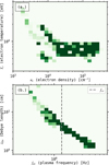 |
Fig. 2 Typical plasma parameters achievable in the plasma chamber. Panel a: plasma density and electron temperature. Panel b: associated plasma frequency and Debye length. The measurements are weighted according to their uncertainty: the brighter the color, the preciser the measurement. The electron cyclotron frequency associated with Earth’s magnetic field is shown as a vertical dashed gray line. |
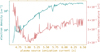 |
Fig. 3 Experimental relation between the measured plasma density, the electron temperature, and the ionization current Ii controlled on the plasma source. |
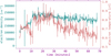 |
Fig. 4 Measurements of the plasma density and electron temperature shown as a function of the time elapsed since the plasma source was turned on. The plasma stabilized with time, with a typical timescale of 30 minutes. |
2.2.2 Plasma stability and experimental repeatability
In this section, we analyze two properties of the plasma generated inside the plasma chamber that are relevant to the design of our experiments: the temporal plasma stability, and the experimental repeatability of the measurements.
First, we analyze the stability of the plasma when the plasma source was turned on. A transient effect was observed for both the plasma density and electron temperature, shown in Fig. 4. To avoid the impact of this transient on our measurements, we waited at least 45 minutes after the plasma source was powered on (i.e., after the plasma was first created) before performing any experiment.
Second, we discuss the repeatability of the plasma produced inside the plasma chamber (i.e., the ability to consistently recreate a plasma of a given density and electron temperature). For this purpose, we introduce another experimental relation between the different properties of the plasma source. Figure 3 shows that the ionization current Ii controls the plasma density. The plasma can also be monitored using another proxy current, namely the discharge current Id, which is measured between the ionization filament and the walls of the ionization chamber. In the absence of a plasma, the two elements are not electrically connected, so that Id = 0. Instead, in the presence of a plasma in the ionization chamber, a discharge current Id ≠ 0 is carried by the plasma. The experimental relation observed between these two currents is shown in Fig. 5. A given (experimentally imposed) ionization current Ii can correspond to different (measured) discharge currents Id, as shown by the several oblique lines in Fig. 5. The reason for this experimental behavior is not currently understood. Therefore, it is not possible to reliably retrieve the same plasma conditions using a given Ii. In other words, measurement repeatability is affected by the lack of control of the discharge current when imposing a given ionization current. To prevent this effect from impacting our experiments, we chose to perform diagnostics of the plasma every time we changed Ii using a Langmuir probe instead of directly relying on a plasma source calibration.
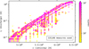 |
Fig. 5 Relation between the ionization current Ii and the discharge current Id measured in the plasma source of the plasma chamber. A total number of 146 245 measurements were used. |
2.2.3 Magnetic field inside the PEPSO plasma chamber
The Earth’s magnetic field is present inside the plasma chamber with a strength B ≃ 40 μT, corresponding to an electron cyclotron frequency fce ≃ 1.1 MHz (vertical dashed line in Fig. 2). The plasma inside the plasma chamber is therefore to be considered as magnetized. In other words, the ratio fpe/fce is not ≫ 1. The axis of the plasma chamber is oriented parallel to the north-south direction. As a result, the magnetic field lies on a plane that is parallel to the plasma chamber axis (within 5%). The magnetic field is also measured to have a downward inclination of ≃50°, compatible with the expected Earth magnetic field dip inclination (≈60°) at the location of the plasma chamber. In the context of this work, we considered antenna alignments either parallel or perpendicular to the axis of the plasma chamber. Therefore, the antenna directions are either inclined by approximately 50° degrees with respect to the magnetic field or are approximately perpendicular to it.
In the remainder of this paper, including the analysis performed in Sect. 3 and Sect. 4, we assumed a fixed and homogeneous geomagnetic field of 48111.7 nT and a downward inclination of 51°, named BEarth.
2.2.4 Instrumentation inside the PEPSO plasma chamber
We introduce the two plasma diagnostic instruments: a Langmuir probe, and a mutual impedance experiment. The plasma chamber with all the instruments highlighted in color is presented in Fig. 6. The Langmuir probe was positioned on a moving support and is shown in the figure in its extended position.
The Langmuir probe (Impedans company/Langmuir Probe system) is composed of a spherical sensor 5 cm in diameter and an electronics box placed outside the plasma chamber. The sensor is placed on a one-axis translating support, so that it can be placed either close to the mutual impedance experiment or farther away. Having both the Langmuir probe and the mutual impedance experiment sensors located in close vicinity means that they both measure the same plasma. When the mutual impedance measurement was performed, the Langmuir probe was retracted away from the mutual impedance experiment sensors in order to avoid perturbing its measurement. In its retracted position, the Langmuir probe becomes nearly flush with the wall of the plasma chamber. The explanation of how we retrieved the plasma density and electron temperature from the Langmuir probe measurements is provided in Appendix E.
The quadrupolar mutual impedance experiment is composed of two aligned electric antennas, both made of a pair of spherical electrodes with a diameter of 2 cm: a dipolar emitting antenna (E1, E2 in Fig. 6), and a dipolar receiving antenna (R1, R2 in Fig. 6). The distance between E1 and E2 (R1 and R2) was 9 cm (26 cm). This aligned configuration was chosen because it defines a single antenna direction relative to the magnetic field to facilitate the measurement analysis. Pre-amplifiers were connected to both the emitting and receiving antennas to adapt to the cable impedance toward the emitting antenna and to provide high-input impedance from the point of view of the receiving antennas. Their gain, set to 1 for most experiments, can also be increased when the mutual impedance signal is found to be too low. We used a PicoScope 5000D (equipped with an arbitrary signal generator and a digital oscilloscope) to simultaneously produce an alternating potential difference and measure an electric potential, as required in Sect. 2.1. This choice is validated in Appendix D by comparison to other solutions. The PicoScope performed a frequency sweep in the range [100 kHz, 20 MHz], encompassing the electron cyclotron frequency and the plasma frequency expected in the plasma chamber. For each of the frequencies in the sweep, we fixed a total duration for the emitted signal equal to 60 times its period. The relative change from one frequency to the next in the sweep was 1.5%. The amplitude of the emitted signal was 1 V peak to peak. Before reaching the pre-amplifiers, the signal generated by the PicoScope was split in two, and one signal was dephased by 180 degrees; both were finally fed into the emitting antenna pre-amplifiers. The two electrodes of the emitting antenna are therefore at opposite potentials ±V. The signal coming out of the receiving antenna pre-amplifiers was fed into a differential amplifier, so that the final measured signal was a differential (dipolar) measurement (E1-E2). The PicoScope together with the pre-amplifier behaved as a voltage generator.
2.3 Numerical model for mutual impedance experiments in the PEPSO plasma chamber
The experimental procedure detailed in Sect. 2.1 and the setup described in Sect. 2.2 led to the requirements for our instrument model.
The instrument model must take as input the voltage imposed on the emitting antenna and must provide as output the voltage difference between the electrodes of the receiving antenna.
The model must take as inputs the plasma parameters, in particular, the plasma density and electron temperature (assumed to be isotropic).
It must take into account the three-dimensional structure of the mutual impedance experiment, as well as the conductive plasma chamber boundaries.
It must take into account the presence of Earth’s magnetic field, since fpe/fce ≃ 1.
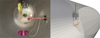
Fig. 6 Left: interior of the PEPSO plasma chamber, with the mutual impedance antennas (orange) and pre-amplifiers (yellow), the Langmuir probe (red), the plasma source (green), and the inlet for the vacuum pumps (violet). The Langmuir probe in the retracted position is hidden in the hole located on the right, at the support base. Right: three-dimensional mesh used to discretize the PEPSO plasma chamber in the DSCD mutual impedance numerical model. The pair of electrodes of the emitting (receiving) antenna are indicated as E1 and E2 (R1, R2).
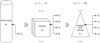
Fig. 7 Hierarchy of our DSCD model. From left to right: DSCD model M, made of a collection of three-dimensional elements En. Each element is described by a triangular mesh composed of a number of triangles Tm.
The emitting voltage amplitude is low enough so that the plasma behavior is considered linear (Bucciantini et al. 2022).
The antennas are small enough so that the electrostatic approximation holds (Dazzi et al. 2025).
At the considered frequencies, the plasma ions are considered as an immobile neutralizing background.
The plasma inside the plasma chamber is considered homogeneous.
The plasma sheath formed around the antenna and the chamber walls is neglected.
Our numerical model used the discrete surface charge distribution (hereafter DSCD) technique (Béghin & Kolesnikova 1998; Kolesnikova & Béghin 1998; Geiswiller 2001; Wattieaux et al. 2019, 2020) to reconstruct the electric charge distribution over all the conducting boundaries (e.g., antennas, metallic elements, and walls) present in the plasma chamber.
The initial step was to discretize the geometry. The three-dimensional model geometry we used is presented in the right panel of Fig. 6. We now describe the construction of the model in more detail. It is illustrated in Fig. 7. The model geometry was composed of an ensemble of elements En with n = 1, ..., N, each of which was considered as a perfect conductor, namely, the antennas, their support system, the pre-amplifier box, and the inner walls of the chamber. Each of these elements was at a potential VEn,
![Mathematical equation: $\[V_{E_n}=V_{S C}+V_{B_n}-i \omega Z_{E_n} Q_n,\]$](/articles/aa/full_html/2026/03/aa54409-25/aa54409-25-eq5.png) (1)
(1)
where VSC is the ground potential, VBn the bias potential imposed on the element, and Qn the total electric charge present on the element. ZEn is the equivalent impedance connecting the element to the bias voltage generator, that is, the impedance of the equivalent Thévenin dipole between the element En and the ground. For space applications, VSC corresponds to the floating potential at frequency ω of the electrically isolated spacecraft in space. VBn is zero for most of the elements, except for the emitting antenna. Thanks to the choice of the electronics used in this work, ZEn was set to zero for all elements, except for the receiving antenna, for which ![Mathematical equation: $\[Z_{E_{n}}=\frac{1}{i \omega C_{R}}\]$](/articles/aa/full_html/2026/03/aa54409-25/aa54409-25-eq6.png) with CR = 15 pF.
with CR = 15 pF.
Each of these conducting elements was discretized with a numerical mesh that defined its surface, where the electric charge was distributed. We used triangular meshes such that a total of Mn triangles made up the element. The total number of triangles was ![Mathematical equation: $\[K=\sum_{n=1}^{N} M_{n}\]$](/articles/aa/full_html/2026/03/aa54409-25/aa54409-25-eq7.png) . We assumed that the electric charge distribution σm was homogeneous over each of the triangles, and we defined the total charge on one triangle as qm,
. We assumed that the electric charge distribution σm was homogeneous over each of the triangles, and we defined the total charge on one triangle as qm,
![Mathematical equation: $\[q_m=\iint_{T_m} \sigma_m d^2 \boldsymbol{s}=\sigma_m T_m,\]$](/articles/aa/full_html/2026/03/aa54409-25/aa54409-25-eq8.png) (2)
(2)
where the surface integration was performed over the triangle Tm. The total charge on one element En is then
![Mathematical equation: $\[Q_n=\sum_{m=1}^{M_n} q_m.\]$](/articles/aa/full_html/2026/03/aa54409-25/aa54409-25-eq9.png) (3)
(3)
The combination of Eqs. (1), (2), (3) provides a relation between the electric potential of each element VEn and the charge distribution qm it carries. Each of the triangles of the model was approximated as a point-like charge, located in the center of the triangle cm and having a charge equal to the total charge distributed on the triangle itself qm. This means that the multipole contributions given by the triangular charge distribution were neglected, and only the monopole contribution was kept. This is validated in Appendix C.
The potential Vm of each of the triangles composing the conducting elements reads
![Mathematical equation: $\[4 \pi \varepsilon_0 V_m=\frac{q_m}{\alpha_m}+\sum_{n=1}^N \sum_{j=1, j \neq m}^{M_n} \frac{q_j}{r_{m j}} \frac{V}{V_0}\left(\boldsymbol{r}_{m j}\right),\]$](/articles/aa/full_html/2026/03/aa54409-25/aa54409-25-eq10.png) (4)
(4)
where
rmj = rm − rj is the vector connecting the center of the triangles m and j,
V/V0 is the potential generated by a point-like charge embedded in the plasma normalized to its value in vacuum, in other words, the problem’s Green function.
![Mathematical equation: $\[\frac{q_{m}}{\alpha_{m}}\]$](/articles/aa/full_html/2026/03/aa54409-25/aa54409-25-eq11.png) is the potential generated by the electric charge that is deposited on the triangle m itself.
is the potential generated by the electric charge that is deposited on the triangle m itself.
In a magnetized plasma, V/V0 reads (Dazzi et al. 2025)
![Mathematical equation: $\[\frac{V}{V_0}=\frac{2 \sqrt{r^2+z^2}}{\pi} \int_0^{+\infty} d k_r \int_0^{+\infty} d k_z \frac{k_r J_0\left(k_r r\right) ~\cos \left(k_z z\right)}{k^2 \varepsilon_L\left(k_r, k_z, \omega\right)} \delta\left(\omega-\omega_e\right),\]$](/articles/aa/full_html/2026/03/aa54409-25/aa54409-25-eq12.png) (5)
(5)
where (r, z) represent the rmj vector in cylindrical coordinates, ωe is the emitting angular frequency, and J0 is the Bessel function of the first kind.
The self-potential ![Mathematical equation: $\[\frac{q_{m}}{\alpha_{m}}\]$](/articles/aa/full_html/2026/03/aa54409-25/aa54409-25-eq13.png) reads
reads
![Mathematical equation: $\[\frac{q_m}{\alpha_m}=\frac{q_m}{T_m} \iint_{T_m} \frac{V}{V_0}\left(\boldsymbol{s}-\boldsymbol{c}_m\right) \frac{1}{\left|\boldsymbol{s}-\boldsymbol{c}_m\right|} d^2 \boldsymbol{s}.\]$](/articles/aa/full_html/2026/03/aa54409-25/aa54409-25-eq14.png) (6)
(6)
The details regarding the calculation of Eq. (6) are given in Appendix A.
In order to conclude the definition of our model, it is useful to update the notation used for the potentials and impedances in Eq. (1). For the potentials, each element En was considered as equipotential, and therefore,
![Mathematical equation: $\[T_m \in E_n \Longrightarrow V_m=V_{E_n}.\]$](/articles/aa/full_html/2026/03/aa54409-25/aa54409-25-eq15.png) (7)
(7)
For the impedances, we defined an impedance matrix Zij as
![Mathematical equation: $\[Z_{i j} \equiv\left\{\begin{array}{l}Z_{E_n} \quad\text { for }\quad T_i, T_j \in E_n \\0 \quad\text { otherwise. }\end{array}\right.\]$](/articles/aa/full_html/2026/03/aa54409-25/aa54409-25-eq16.png) (8)
(8)
The K charges qm and VSC are the K + 1 unknowns to be solved. The combination of Eqs. (1) and (4) leads to a system of K linear equations for the electric charges qm. To close the system, we used the total electric charge conservation,
![Mathematical equation: $\[\sum_{n=1}^N \sum_{j=1}^{M_n} q_m=0,\]$](/articles/aa/full_html/2026/03/aa54409-25/aa54409-25-eq17.png) (9)
(9)
bringing the number of equations to K + 1.
The combination of Eqs. (1), (4), (9) leads to the linear system
![Mathematical equation: $\[\boldsymbol{D} \cdot \boldsymbol{q}=k_0 \boldsymbol{V},\]$](/articles/aa/full_html/2026/03/aa54409-25/aa54409-25-eq18.png) (10)
(10)
where the terms are defined as
![Mathematical equation: $\[\boldsymbol{D} \equiv\left(\begin{array}{cccc}\frac{1}{\alpha_1}+i \omega k_0 Z_{11} & \frac{1}{\left|\boldsymbol{r}_1-\boldsymbol{r}_2\right|} \frac{V}{V_0}+i \omega k_0 Z_{12} & \ldots & 1 \\\frac{1}{\left|\boldsymbol{r}_2-\boldsymbol{r}_1\right|} \frac{V}{V_0}+i \omega k_0 Z_{21} & \frac{1}{\alpha_2}+i \omega k_0 Z_{22} & \ldots & 1 \\\ldots & \ldots & \ldots & 1 \\1 & 1 & \ldots & 0\end{array}\right)_{(K+1) \times(K+1)}\]$](/articles/aa/full_html/2026/03/aa54409-25/aa54409-25-eq19.png) (11)
(11)
and
![Mathematical equation: $\[\boldsymbol{q} \equiv\left(\begin{array}{c}q_1 \\q_2 \\\ldots \\-k_0 V_{S C}\end{array}\right)_{(K+1)} \quad, \quad \boldsymbol{V} \equiv\left(\begin{array}{c}V_{B_1} \\V_{B_2} \\\ldots \\0\end{array}\right)_{(K+1)},\]$](/articles/aa/full_html/2026/03/aa54409-25/aa54409-25-eq20.png) (12)
(12)
with k0 = 4πε0. We used the LU decomposition to factor the matrix D in Eq. (10) and solve for the charges qm and the potential VSC. From Eq. (1) and the charges qm, we finally derived the electric potentials on each of the model elements. We present the validation of this model in Appendix B for a variety of cases with and without a plasma.
The computation we just described was performed for each of the emission frequencies composing a mutual impedance spectrum. The modeled mutual impedance spectrum was obtained from the potential difference between the receiving antennas and was computed for each frequency.
3 Measurements of mutual impedance experiments in a laboratory plasma
In this section we present our measurements. The plasma density was progressively increased by increasing the ionization current Ii, while performing a mutual impedance measurement and a Langmuir probe I–V sweep iteratively, with the experimental setup shown in Fig. 6 and described in Sect. 2.2. We present the totality of our mutual impedance measurements in the form of a dynamic spectrum in Fig. 8 for the amplitude of the mutual impedance, normalized to vacuum and shown in dB. The horizontal axis shows the ionization current, to be considered as an experimental proxy for the plasma density. To facilitate the interpretation of the results, we also chose to normalize each spectrum to its maximum value in panels b and d. The measurements in panels a and b (c and d) were obtained with the antenna axis perpendicular (parallel) to the plasma chamber axis.
A few representative examples of mutual impedance spectra from these measurements are shown in Fig. 9, where we show in the upper row (lower row) measurements obtained with the antenna perpendicular (parallel) to the axis of the plasma chamber (as in Fig. 8). The plasma density also increases from left to right. The characteristic frequencies of a magnetized mutual impedance measurement are shown in Fig. 9 as colored vertical lines, namely: the harmonics of the electron cyclotron frequency n · fce, the upper hybrid frequency ![Mathematical equation: $\[f_{u h}=\sqrt{f_{p e}^{2}+f_{c e}^{2}}\]$](/articles/aa/full_html/2026/03/aa54409-25/aa54409-25-eq21.png) , and the series of fqn frequencies. The upper hybrid frequency fuh was obtained from the measured plasma density and BEarth. The electron cyclotron frequency was also obtained from BEarth. The fqn frequencies were obtained by using the Hamelin diagram (Pottelette 1981) constructed from the numerical solution of the linear plasma dispersion relation (Rönnmark 1982).
, and the series of fqn frequencies. The upper hybrid frequency fuh was obtained from the measured plasma density and BEarth. The electron cyclotron frequency was also obtained from BEarth. The fqn frequencies were obtained by using the Hamelin diagram (Pottelette 1981) constructed from the numerical solution of the linear plasma dispersion relation (Rönnmark 1982).
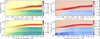 |
Fig. 8 Two sets of measurements of mutual impedance spectra. The ionization current is on the horizontal axis, the frequency on the vertical axis, and we show the amplitude of the mutual impedance in color. Panels (a) and (b) (c and d): measurements taken with the antenna perpendicular (parallel) to the axis of the plasma chamber. Panel (a) and (c) (b and d) show measurements that were normalized to the mutual impedance in vacuum (to their maximum value, for illustration purposes). |
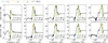 |
Fig. 9 Representative set of magnetized mutual impedance amplitude spectra, normalized to vacuum, in the upper (lower) row with the antenna perpendicular (parallel) to the axis of the plasma chamber. The plasma density increases from left to right. The ionization filament current Ii is indicated in each panel, with the ratio of the plasma to electron cyclotron frequency fpe/fce. The following characteristic frequencies are shown as vertical lines: the harmonics of the electron cyclotron frequency, the upper hybrid frequency, and the series of fqn frequencies. |
4 Analysis of mutual impedance measurements in a magnetized plasma
In this section, we describe the analysis of the mutual impedance measurements from Sect. 3.
Figure 8 shows that the frequency of the maximum mutual impedance spectrum increases as the plasma density increases (i.e., for larger Ii). This is consistent with the fact that the maximum is close to the local upper hybrid frequency fuh. The alignment between the upper hybrid frequency and the maximum of the upper hybrid frequency is also shown in Fig. 9. This reinforces the conclusions that fuh is located close to the absolute maximum of the mutual impedance spectrum.
The amplitude of the absolute maximum close to fuh is also expected to increase as the Debye length decreases. This behavior is known for an unmagnetized plasma (Gilet et al. 2019) and has only been proven numerically in the magnetized case (Dazzi et al. 2025). This trend is shown experimentally in panels a and c of Fig. 8, where, as the density increases (increasing Ii), the Debye length decreases because the electron temperature is approximately constant (Fig. 2). This trend is also observed in Fig. 9. We confirm the previous numerical predictions of Dazzi et al. (2025) experimentally in this way.
The mutual impedance spectrum is known to have local minima close to the harmonics of the electron cyclotron frequency n · fce (Dazzi et al. 2025). This is because the wavelength of the electron Bernstein waves that are excited by the mutual impedance experiment tends to either zero or infinity at these frequencies. These wavelengths are not measurable by the receiving electric antenna and therefore appear as a minimum. This behavior is also visible in the measurements presented in Fig. 9, where fce and 2fce are both close to local minima in the mutual impedance spectra.
Electron Bernstein waves also cause the local maxima in Fig. 9. These local maxima are located at the fqn frequencies, defined as the frequencies at which electron Bernstein waves have zero group velocity for f ≥ fuh. We can also define the fqn as the frequencies that delimit the Bernstein mode forbidden bands, meaning that for fqn < f < (n + 1) · fce, no Bernstein modes exist. The typical wavelengths of the electron Bernstein waves at zero group velocity, oscillating at the so-called fqn frequencies, is ≃60 Debye lengths at most. The wavelengths are comparable with the diameter of the plasma chamber (1m). We still expect the antenna to be able to emit and receive these wavelengths, as illustrated, for example, by Wattieaux et al. (2019).
In the high-frequency limit f ≫ fuh, the mutual impedance tends to its value in vacuum, meaning that the normalized spectrum presented in Fig. 9 tends to one. This behavior validates the normalization procedure of our measurements.
We now focus on obtaining a plasma diagnostic from magnetized mutual impedance measurements. We also compare the diagnostics obtained for the plasma density ne and electron temperature Te with those provided independently by a Langmuir probe. We remark that in the remainder of this section, we only use the measurements obtained with ionization current Ii ≥ 5 A. In this way, for all measurements, the Debye length is ≃2.5 cm at most, so that the plasma sheath is not larger than the separation between the antennas. We derived the plasma density and electron temperature from the measured mutual impedance spectra by comparison (best fit) with the instrument model defined in Sect. 2.3. We followed a two-step approach that had the objective of successively refining the measurements of the plasma parameters while at the same time avoiding local minima in the best-fit determination. We began by finding the best fit between the measurements and the instrument model in the unmagnetized limit, assuming a Maxwellian distribution for the electrons. The three-dimensional mesh we used was composed of 3812 triangular elements. We employed the Levenberg-Marquardt algorithm (Watson 1978), and the two free parameters in the best fit were the plasma density and the electron temperature. In this procedure, we need to specify a first guess for each of the two free parameters. For the plasma density first guess, we identified the maximum of the spectrum and assumed that it was the upper hybrid frequency fuh. We derived the density from fuh assuming that the magnetic field strength was BEarth. For the electron temperature first guess, we chose the temperature measured by the Langmuir probe. This unmagnetized best fit provides an initial approximation of the plasma density and electron temperature, which we named ![Mathematical equation: $\[n_{e}^{unmag.}\]$](/articles/aa/full_html/2026/03/aa54409-25/aa54409-25-eq22.png) and
and ![Mathematical equation: $\[T_{e}^{unmag.}\]$](/articles/aa/full_html/2026/03/aa54409-25/aa54409-25-eq23.png) , respectively.
, respectively.
We used ![Mathematical equation: $\[n_{e}^{unmag.}\]$](/articles/aa/full_html/2026/03/aa54409-25/aa54409-25-eq24.png) and
and ![Mathematical equation: $\[T_{e}^{unmag.}\]$](/articles/aa/full_html/2026/03/aa54409-25/aa54409-25-eq25.png) as initial guesses for finding the best fit between the measurements and the magnetized instrument model. We employed the same approach as before, and we again left the plasma density and electron temperature as free parameters. In this case, we also needed to specify the magnetic field amplitude and direction. Because of the implementation of the numerical calculation of V/V0 in Eq. (5), we needed to define the ratio of the plasma to electron cyclotron frequency fpe/fce. Therefore, we started by computing V/V0 over an ensemble of values of fpe/fce. For each of the measured mutual impedance spectra, we computed the ratio of fpe/fce using
as initial guesses for finding the best fit between the measurements and the magnetized instrument model. We employed the same approach as before, and we again left the plasma density and electron temperature as free parameters. In this case, we also needed to specify the magnetic field amplitude and direction. Because of the implementation of the numerical calculation of V/V0 in Eq. (5), we needed to define the ratio of the plasma to electron cyclotron frequency fpe/fce. Therefore, we started by computing V/V0 over an ensemble of values of fpe/fce. For each of the measured mutual impedance spectra, we computed the ratio of fpe/fce using ![Mathematical equation: $\[n_{e}^{unmag.}\]$](/articles/aa/full_html/2026/03/aa54409-25/aa54409-25-eq26.png) and BEarth. We chose the closest value of fpe/fce of the available values and performed the fit using this fixed value of fpe/fce. This second best fit provided the final determination of the plasma density and electron temperature, named
and BEarth. We chose the closest value of fpe/fce of the available values and performed the fit using this fixed value of fpe/fce. This second best fit provided the final determination of the plasma density and electron temperature, named ![Mathematical equation: $\[n_{e}^{mag.}\]$](/articles/aa/full_html/2026/03/aa54409-25/aa54409-25-eq27.png) and
and ![Mathematical equation: $\[T_{e}^{mag.}\]$](/articles/aa/full_html/2026/03/aa54409-25/aa54409-25-eq28.png) . A set of representative examples of the best fits is presented in Appendix F.
. A set of representative examples of the best fits is presented in Appendix F.
We compare the density and temperature measurements obtained by the mutual impedance experiment ![Mathematical equation: $\[n_{e}^{mag.}\]$](/articles/aa/full_html/2026/03/aa54409-25/aa54409-25-eq29.png) and
and ![Mathematical equation: $\[T_{e}^{mag.}\]$](/articles/aa/full_html/2026/03/aa54409-25/aa54409-25-eq30.png) with those obtained by the Langmuir probe
with those obtained by the Langmuir probe ![Mathematical equation: $\[n_{e}^{L P}\]$](/articles/aa/full_html/2026/03/aa54409-25/aa54409-25-eq31.png) and
and ![Mathematical equation: $\[T_{e}^{L P}\]$](/articles/aa/full_html/2026/03/aa54409-25/aa54409-25-eq32.png) in Fig. 10. The top panel shows the density and temperature ratios
in Fig. 10. The top panel shows the density and temperature ratios ![Mathematical equation: $\[n_{e}^{L P} / n_{e}^{mag.}\]$](/articles/aa/full_html/2026/03/aa54409-25/aa54409-25-eq33.png) and
and ![Mathematical equation: $\[T_{e}^{L P} / T_{e}^{mag.}\]$](/articles/aa/full_html/2026/03/aa54409-25/aa54409-25-eq34.png) as a function of Ii, in other words, as a function of the increasing plasma density. The bottom panel shows a direct comparison of the densities
as a function of Ii, in other words, as a function of the increasing plasma density. The bottom panel shows a direct comparison of the densities ![Mathematical equation: $\[n_{e}^{L P}\]$](/articles/aa/full_html/2026/03/aa54409-25/aa54409-25-eq35.png) versus
versus ![Mathematical equation: $\[n_{e}^{mag.}\]$](/articles/aa/full_html/2026/03/aa54409-25/aa54409-25-eq36.png) . (bottom left) and temperatures
. (bottom left) and temperatures ![Mathematical equation: $\[T_{e}^{L P}\]$](/articles/aa/full_html/2026/03/aa54409-25/aa54409-25-eq37.png) versus
versus ![Mathematical equation: $\[T_{e}^{mag.}\]$](/articles/aa/full_html/2026/03/aa54409-25/aa54409-25-eq38.png) (bottom right), obtained with the two independent measurement methods. The density and temperature measurements are both compatible within the measurement uncertainties. While the density variation spans over one order of magnitude, the variation in the electron temperature is relatively small, about a factor of 2. These measurements show (i) the consistency of the diagnostic performed by the two instrumental methods and (ii) validated the mutual impedance model developed in this paper for magnetized plasmas.
(bottom right), obtained with the two independent measurement methods. The density and temperature measurements are both compatible within the measurement uncertainties. While the density variation spans over one order of magnitude, the variation in the electron temperature is relatively small, about a factor of 2. These measurements show (i) the consistency of the diagnostic performed by the two instrumental methods and (ii) validated the mutual impedance model developed in this paper for magnetized plasmas.
Fig. F.1 shows that the experimental measurements obtained in the presence of a certain level of plasma inhomogeneity (i.e., for the lowest values of the plasma density, and thus, for the longest Debye lengths) agree with the model derived under the assumption of an homogeneous plasma. This suggests that the model is actually robust to the presence of plasma inhomogeneities, at least in the regime of a ratio of the Debye length (i.e., smaller than 2.5 cm) over antenna distance (i.e., 9 cm) smaller than 4, as this is the regime we investigated.
5 Conclusions and perspective
We presented a quantitative comparison between mutual impedance experiments in a magnetized plasma and an instrument model that is able to reproduce these measurements. This comparison enabled us for the first time to obtain a diagnostic for the plasma density and electron temperature from mutual impedance experiments in a magnetized plasma, such as those encountered in our Solar System. We reached this result by developing two tools, one numerical and one experimental tool.
On the one hand, the numerical tool is a flexible numerical model of mutual impedance experiments in magnetized space plasma. It is based on, first, a generalization of the modeling used to interpret the mutual impedance measurements obtained by the Rosetta RPC/MIP experiment (Wattieaux et al. 2019), and second, on the numerical computation of the plasma Green function presented by Dazzi et al. (2025). The model takes into account (i) the instrument geometry and the surrounding experimental geometry setup and (ii) the kinetic nature of the plasma electron dynamics in a homogeneous magnetized plasma.
On the other hand, the experimental tool is a laboratory plasma chamber (Bucciantini et al. 2023) containing two plasma instruments: a mutual impedance experiment, and a Langmuir probe to provide independent plasma diagnostics. We characterized the plasma chamber properties, including (i) the range of available plasma parameters, (ii) the stability, and (iii) the repeatability of the generated plasma. With this setup, we performed mutual impedance and Langmuir probe measurements in a controlled plasma environment.
We achieved a qualitative and quantitative interpretation of the acquired mutual impedance spectra to show their dependence on the plasma density, and in particular, on the ratio fpe/fce. As expected, we observed spectral features (Dazzi et al. 2025) at the upper hybrid frequency (local maximum), harmonics of the electron cyclotron frequency (local minima), and so-called electron Bernstein fqn frequencies (local maxima). We observed and explained their respective strengths for low (fpe/fce ≳ 3.5) to high (fpe/fce ≲ 0.5) plasma densities. Mutual impedance experiments were experimentally investigated for the first time in this parameter range.
Our mutual impedance numerical model is able to reproduce the measured mutual impedance spectra from the plasma chamber experiments, which experimentally validated the model. In particular, one of the hypotheses we used to construct the numerical model was the electrostatic hypothesis ∂tB = 0. This hypothesis, conjectured in previous works (Chasseriaux et al. 1972; Kuehl 1974; Pottelette 1981) and justified theoretically by Dazzi et al. (2025), is based on the fact that the wavelength of electromagnetic waves is far larger than that of electrostatic ones, so that their effect on the mutual impedance spectrum is thought to be negligible. We indeed showed that no effect associated with electromagnetic waves is required to reproduce the measured mutual impedance spectra, and we therefore validated this approximation a posteriori and experimentally. This is central in our modeling approach and in the interpretation of the experimental results.
We employed the numerical model we developed to extract a diagnostic for the plasma density and the electron temperature from our experimental plasma chamber measurements by comparing them to predictions from our numerical model. Practically, by finding the best-fit between the model and the measurements, we were able to determine the plasma density and electron temperature. We compared these parameters with those measured independently by the Langmuir probe. The plasma density and electron temperature obtained by these two independent instruments were compatible within the measurement uncertainty. This proves experimentally that it is possible to retrieve the plasma density and electron temperature in a magnetized plasma from mutual impedance experiments.
The model we used is based on strong assumptions: that the plasma density, temperature, and magnetic field are homogeneous in the region surrounding the instrument. This is hardly achievable in a plasma chamber, and in particular, around an antenna in space because of the plasma sheath. We estimate (measurements not shown here) that the density and temperature might vary by up to a factor of 5 in the plasma surrounding the instruments. Nonetheless, it is remarkable that the model results are coherent even though the plasma is inhomogeneous inside the plasma chamber. This further illustrates the robustness of the diagnostic.
This work also illustrates that the development of an instrument used for space plasma diagnostics, such as a mutual impedance experiment, strongly benefits from testing in a controlled plasma environment, such as a plasma chamber.
We plan to use the modeling framework we developed and validated here in the context of future space missions, such as BepiColombo and JUICE, in the magnetosphere of Mercury, Jupiter, and Ganymede for the mutual impedance experiments PWI/AM2P and RPWI/MIME, respectively. In the case of a space instrument onboard of a spacecraft, a relevant subset or the entire spacecraft geometry will be implemented instead of the plasma chamber geometry.
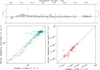 |
Fig. 10 Comparison results of the mutual impedance and Langmuir probe. Top: ratio of the plasma density |
![Mathematical equation: $\[n_{e}^{L P}\left(n_{e}^{M I}\right)\]$](/articles/aa/full_html/2026/03/aa54409-25/aa54409-25-eq39.png)
![Mathematical equation: $\[T_{e}^{L P}\left(T_{e}^{M I}\right)\]$](/articles/aa/full_html/2026/03/aa54409-25/aa54409-25-eq40.png)
![Mathematical equation: $\[n_{e}^{M I}\]$](/articles/aa/full_html/2026/03/aa54409-25/aa54409-25-eq41.png)
![Mathematical equation: $\[n_{e}^{L P}\]$](/articles/aa/full_html/2026/03/aa54409-25/aa54409-25-eq42.png)
![Mathematical equation: $\[T_{e}^{M I}\]$](/articles/aa/full_html/2026/03/aa54409-25/aa54409-25-eq43.png)
![Mathematical equation: $\[T_{e}^{L P}\]$](/articles/aa/full_html/2026/03/aa54409-25/aa54409-25-eq44.png)
Acknowledgements
The authors benefited from the use of the computation cluster made available by the CaSciModOT federation at the Centre de Calcul Scientifique in the Centre-Val de Loire region. The work performed at LPC2E and in particular the development of the PEPSO plasma chamber is supported by the CNES APR (Appel à Propositions de Recherche scientifique).
References
- Bahnsen, A., Jespersen, M., Ungstrup, E., et al. 1988, Phys. Scr., 37, 469 [Google Scholar]
- Beghin, C. 1971, Space Res. XI, 1, 1071 [Google Scholar]
- Benkhoff, J., van Casteren, J., Hayakawa, H., et al. 2010, Planet. Space Sci., 58, 2 [NASA ADS] [CrossRef] [Google Scholar]
- Blackwell, D. D., Walker, D. N., & Amatucci, W. E. 2005, Rev. Sci. Instrum., 76, 023503 [Google Scholar]
- Bucciantini, L., Henri, P., Wattieaux, G., et al. 2022, J. Geophys. Res.: Space Phys., 127, e2022JA030813 [Google Scholar]
- Bucciantini, L., Henri, P., Dazzi, P., et al. 2023, J. Geophys. Res.: Space Phys., 128, e2022JA031055 [Google Scholar]
- Béghin, C., & Kolesnikova, E. 1998, Radio Sci., 33, 503 [Google Scholar]
- Béghin, C., Berthelier, J., Debrie, R., et al. 1982, Adv. Space Res., 2, IN5 [Google Scholar]
- Chasseriaux, J. M., R. Debrie, & C. Renard. 1972, J. Plasma Phys., 8, 231 [Google Scholar]
- Dazzi, P., Henri, P., Bucciantini, L., et al. 2025, A&A, 696, A39 [NASA ADS] [CrossRef] [EDP Sciences] [Google Scholar]
- Decreau, P. M. E., Beghin, C., & Parrot, M. 1978, Space Sci. Rev., 22, 581 [Google Scholar]
- Diaconis, P., & Miclo, L. 2011, Combinatorics Probab. Comput., 20, 213 [Google Scholar]
- Gargioni, E., & Grosswendt, B. 2008, Rev. Mod. Phys., 80, 451 [Google Scholar]
- Geiswiller, J. 2001, PhD thesis, Université d’Orléans, Orléans, France [Google Scholar]
- Gilet, N., Henri, P., Wattieaux, G., et al. 2019, Front. Astron. Space Sci., 6, 16 [NASA ADS] [Google Scholar]
- Grasset, O., Dougherty, M., Coustenis, A., et al. 2013, Planet. Space Sci., 78, 1 [CrossRef] [Google Scholar]
- Grosso, G., & Pastori Parravicini, G. 2014, Solid State Physics, 2nd edn. (Amsterdam: Academic Press, an imprint of Elsevier) [Google Scholar]
- Haeusler, B., Haerendel, G., Bauer, O., et al. 1979, Sounding Rocket Program Magnetosphere. Project PORCUPINE, Final report, Max-Planck-Inst. fuer Physik und Astrophysik, Garching (Germany, F.R.). Inst. fuer Extraterrestrische Physik [Google Scholar]
- Hamelin, M., Béghin, C., Grard, R., et al. 2007, Planet. Space Sci., 55, 1964 [NASA ADS] [Google Scholar]
- Jaeger, E. F., Berry, L. A., & Batchelor, D. B. 1991, J. Appl. Phys., 69, 6918 [Google Scholar]
- Karlsson, T., Kasaba, Y., Wahlund, J.-E., et al. 2020, Space Sci. Rev., 216, 132 [Google Scholar]
- Kasaba, Y., Kojima, H., Moncuquet, M., et al. 2020, Space Sci. Rev., 216, 65 [NASA ADS] [CrossRef] [Google Scholar]
- Kaufman, H. R., Cuomo, J. J., & Harper, J. M. E. 1982, J. Vac. Sci. Technol., 21, 725 [Google Scholar]
- Kolesnikova, E., & Béghin, C. 1998, Radio Sci., 33, 491 [Google Scholar]
- Kraus, J. D. 1997, Antennas, 2nd edn. (Tata McGraw-Hill) [Google Scholar]
- Kuehl, H. H. 1974, Phys. Fluids, 17, 1275 [Google Scholar]
- Laframboise, J. G. 1966, Report No. 100, University of Toronto, Institute for Aerospace Studies, Fort Belvoir, VA [Google Scholar]
- Lobbia, R. B., & Beal, B. E. 2017, J. Propuls. Power, 33, 566 [Google Scholar]
- Meyer-Vernet, N., & Perche, C. 1989, J. Geophys. Res., 94, 2405 [NASA ADS] [CrossRef] [Google Scholar]
- Miyake, Y. 2009, PhD thesis, Kyoto University, Kyoto [Google Scholar]
- Perraut, S., De Feraudy, H., Roux, A., et al. 1990, J. Geophys. Res.: Space Phys., 95, 5997 [Google Scholar]
- Pottelette, R. 1981, Phys. Fluids, 24, 1517 [Google Scholar]
- Reichert, B., & Ristivojevic, Z. 2020, Phys. Rev. Res., 2, 013289 [Google Scholar]
- Rönnmark, K. 1982, WHAMP – Waves in Homogeneous Anisotropic Multicomponent Plasmas, 179 (Kiruna: Kiruna Geophysical Institute) [Google Scholar]
- Snodgrass, C., & Jones, G. H. 2019, Nat. Commun., 10, 5418 [NASA ADS] [CrossRef] [Google Scholar]
- Spencer, E., Clark, D., & Vadepu, S. K. 2019, IEEE Trans. Plasma Sci., 47, 1322 [Google Scholar]
- Storey, L. R. O., Aubrey, M. P., & Meyer, P. 1969, in Plasma Waves in Space and in the Laboratory, 1 (Roeros, Norway: New York American Elsevier Publishing Co.), 303 [Google Scholar]
- Trotignon, J. G., Michau, J. L., Lagoutte, D., et al. 2007, Space Sci. Rev., 128, 713 [NASA ADS] [CrossRef] [Google Scholar]
- Wahlund, J.-E., Bergman, J. E. S., Åhlén, L., et al. 2025, Space Sci. Rev., 221, 1 [Google Scholar]
- Watson, G. A. 1978, Numerical Analysis: Proceedings of the Biennial Conference Held at Dundee, June 28-July 1 1977, Lecture Notes in Mathematics Ser No. v. 630 (Berlin, Heidelberg: Springer Berlin / Heidelberg) [Google Scholar]
- Wattieaux, G., Gilet, N., Henri, P., Vallières, X., & Bucciantini, L. 2019, A&A, 630 [Google Scholar]
- Wattieaux, G., Henri, P., Gilet, N., Vallières, X., & Deca, J. 2020, A&A, 638 [Google Scholar]
Appendix A Computation of the DSCD α parameter
In this section we detail how we compute the αm parameter by solving numerically the integral of Eq. 6. This computation is performed differently, depending on whether a plasma is present or not.
In the absence of a plasma V/V0 = 1, so that the computation of α depends only on the shape of the triangle used to define the mesh element Tm. For ease of reference, we rewrite the definition of αm in the absence of plasma here:
![Mathematical equation: $\[\frac{1}{\alpha_m}=\frac{1}{T_m} \iint_{T_m} \frac{1}{\left|\boldsymbol{s}-\boldsymbol{c}_m\right|} d^2 \boldsymbol{s}.\]$](/articles/aa/full_html/2026/03/aa54409-25/aa54409-25-eq45.png) (A.1)
(A.1)
The center cm is chosen to be its barycenter. We compare three different techniques used to compute αm in Eq. A.1, that we name the “sing_int,” “gilet,” and “wattx” techniques.
We start from the “sing_int” technique, by observing that the surface integral in Eq. (A.1) reads
![Mathematical equation: $\[\iint_{T_m} \frac{1}{\left|\boldsymbol{s}-\boldsymbol{c}_m\right|} d^2 \boldsymbol{s}=\sum_{t=1}^3 \iint_{T_m^t} \frac{1}{\left|\boldsymbol{s}-\boldsymbol{c}_m\right|} d^2 \boldsymbol{s}=\sum_{t=1}^3 \int_0^{\Theta} \int_0^{r(\theta)} d r d \theta,\]$](/articles/aa/full_html/2026/03/aa54409-25/aa54409-25-eq46.png) (A.2)
(A.2)
where we divided the triangle Tm in three smaller triangles ![Mathematical equation: $\[T_{m}^{t}\]$](/articles/aa/full_html/2026/03/aa54409-25/aa54409-25-eq47.png) (as shown in Fig. A.1), each sharing two vertices with Tm and having cm as the last vertex. The angle Θ is the angular aperture of each of the smaller triangles. The surface integral is computed in polar coordinates (r, θ) on each of the
(as shown in Fig. A.1), each sharing two vertices with Tm and having cm as the last vertex. The angle Θ is the angular aperture of each of the smaller triangles. The surface integral is computed in polar coordinates (r, θ) on each of the ![Mathematical equation: $\[T_{m}^{t}\]$](/articles/aa/full_html/2026/03/aa54409-25/aa54409-25-eq48.png) , and reads
, and reads
![Mathematical equation: $\[\int_0^{\Theta} \int_0^{r(\theta)} d r d \theta=\int_0^{\Theta} \frac{q}{\sin~ \theta-m ~\cos~ \theta} d \theta,\]$](/articles/aa/full_html/2026/03/aa54409-25/aa54409-25-eq49.png) (A.3)
(A.3)
where we used the fact that r sin θ = y = m · x + q, with the parameters m and q defining the line passing through two corners of ![Mathematical equation: $\[T_{m}^{t}\]$](/articles/aa/full_html/2026/03/aa54409-25/aa54409-25-eq50.png) as described in Fig. A.1. The one-dimensional integral over θ is computed numerically.
as described in Fig. A.1. The one-dimensional integral over θ is computed numerically.
The “gilet” technique is derived from Gilet et al. (2019). In order to compute the surface integral in Eq. A.1, the triangle is subdivided into six sub-triangles of equal areas, as presented in the “gilet” panel of Fig. A.1. The distance between the center of such sub-triangles ci and the center of the original triangle cm is di, and therefore
![Mathematical equation: $\[\alpha_m=\frac{6}{\sum_{i=1}^6 d_i^{-1}}.\]$](/articles/aa/full_html/2026/03/aa54409-25/aa54409-25-eq51.png) (A.4)
(A.4)
We describe the last approach, named the “wattx” technique, and that is derived from the work of Wattieaux et al. (2019). As done in the “gilet” technique, the triangle is subdivided into smaller triangles. The longest side of the triangle is defined as lmax. The triangle is then subdivided recursively by selecting the longest side and splitting it into two if it is longer then lmax./n, generating two sub-triangles. This procedure is repeated to the point when all triangles have their longest side smaller than lmax./n. Such a subdivision, obtained with n = 5, is presented in the “wattx” panel of Fig. A.1. Defining the distance between the center of each of the sub-triangles and the center of the original triangle di and the surface of each of the sub-triangles Si, the final expression for αm is
![Mathematical equation: $\[\alpha_m=\frac{T_m}{\sum_i S_i d_i^{-1}}.\]$](/articles/aa/full_html/2026/03/aa54409-25/aa54409-25-eq52.png) (A.5)
(A.5)
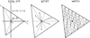 |
Fig. A.1 Subdivision of a triangle mesh element Tm used to compute the αm of Eq. A.1, using one of the three different techniques: “sing_int,” “gilet,” or “wattx.” |
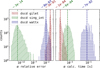 |
Fig. A.2 Left: Relative error obtained by the calculation of the αm parameter Eq. A.1 using different techniques. Right: Computation time for each technique. The histograms are computed using 5000 sample triangles, randomly generated. |
We compare the results of the computation of the αm parameter. We generate an ensemble of 5000 triangles with random shapes, and we compute the αm parameter for each using the three “sing_int,” “gilet,” and “wattx” techniques, as well as by computing the parameter directly from Eq. A.1. The relative uncertainty between the three techniques and the correct result are presented in Fig. A.2 as histograms. In the same figure, we also present the computation time for each of the techniques, also as histograms. We highlight here that the most precise technique is the “sing_int,” which also does not require a considerably long computational time.
In the presence of a plasma, V/V0 is given by the numerical calculation of Eq. 5. This means that in the calculation of the αm parameter depends on both: (i) the shape of the Tm triangle, and (ii) the value of the potential V/V0. As a result, a derivation as the one that leads to Eq. A.3 using the “sing_int” approach is not applicable. The technique we employ in this case therefore follows the approach of the “gilet” technique. In this case, we obtain
![Mathematical equation: $\[\alpha_m=\frac{6}{\sum_{i=1}^6 \frac{1}{d_i} \frac{V}{V_0}\left(\boldsymbol{c}_i-\boldsymbol{c}_m\right)},\]$](/articles/aa/full_html/2026/03/aa54409-25/aa54409-25-eq53.png) (A.6)
(A.6)
where the potential V/V0 is computed as a function of both: the distance between the center of the six sub-triangles and the center of the original triangle |ci − cm|, and the direction of ci − cm relative to the magnetic field.
Appendix B Validation of the numerical implementation of the DSCD technique
In this section we present a number of validations of the implementation of the DSCD technique.
Appendix B.1 Determination of the triangular mesh quality
We present a method to determine the quality of the mesh used in our DSCD approach. We also present an application of this technique to the three-dimensional model used to interpret the measurements presented in this paper.
The DSCD technique requires the definition of a numerical mesh that represents the conductive surfaces present in our experiment, as detailed in Sect. 2.3. In this work, we use triangular meshes. In order for a numerical mesh to be suitable for our DSCD technique, it needs to meet at least two conditions. First, it needs to accurately describe the geometry, meaning that the resolution of the mesh must be low enough as to reproduce the surface details down to the size of the Debye length. This condition is validated when constructing the model, as the Debye length (or at least its order of magnitude) is known. Second, the mesh triangles should be as close as possible to equilateral. This is because each triangle is approximated in the DSCD technique as a point-like charge, located in the center of the triangle. In other words, the multipole expansion of the potential emitted by the triangular charge distribution is truncated to its first term. The moments of order higher than one (the dipole and quadrupole, for example) are omitted, and they are larger if the charge distribution is less close to an equilateral triangle. In the rest of this section, we show how to reliably check that this second (equilateral triangles) condition is met.
We define the procedure that we use to define a standard shape for any triangle in the mesh, in order to be able to compare them. This procedure is composed of a succession of steps, detailed below. We start from a generic triangle in three-dimensional space. Without loss of generality, we place ourselves in the plane containing the triangle. We normalize the longest side of the triangle to one. We align such side with the horizontal axis. If necessary, we flip the triangle around the vertical axis so that its shortest side is on the left. With this procedure, we obtain a triangle of the same type as the one shown in Fig. B.1. The coordinates of the point (εX, εY) of a triangle as the one in Fig. B.1 define uniquely the shape of the original triangle.
In order to evaluate the quality of the triangular mesh used in our DSCD model, is it sufficient to represent all the points (εX, εY), each corresponding to the one triangular mesh element. If the points are all close to the upper limit of the shaded region of Fig. B.1, this means that all the triangles are approximately equilateral, and therefore the mesh is of reasonable quality. If the points are close to the bottom, εX ≫ εY the triangles are all flattened out, and therefore the mesh is not of acceptable quality. We now present two examples of such an analysis.
We start with an example of a mesh of reasonable quality. The mesh we analyze is the one we use to model the mutual impedance experiments inside the plasma chamber, presented in Fig. 6. The points (εX, εY) for this mesh are presented in Fig. B.2 as a scatter plot, and their accumulated distribution along the X and Y directions are presented as histograms on the sides. All the points are located in the upper region of the plot (in green), meaning that the mesh is appropriate for the DSCD technique.
We present an example of a mesh that would not be suitable to the DSCD technique. We take as a mesh obtained from a single triangle that is then subdivided progressively, following the approach close to the one of the barycentric subdivision. The subdivision of one triangle is presented in Fig. B.1, where the sub-triangles obtained from the subdivisions are indicated by T1, T2, T3. Such subdivision is then repeated on all the triangles, recursively. Such a method can be used to increase the spatial resolution of the mesh, but this is done at the expense of the mesh quality. After eight steps, the mesh quality is severely deteriorated, as visible in Fig. B.3. We recognize that in this case, most of the triangles lie at the bottom of the (εX, εY) (in red), meaning that they are not equilateral and instead flattened out. This behavior is expected, as discussed in Diaconis & Miclo (2011).
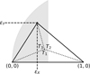 |
Fig. B.1 Definition of the coordinates of the point (εX, εY) that is used to present the quality of the mesh triangles for the DSCD technique. |
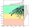 |
Fig. B.2 Mesh quality as defined in Appendix B for the numerical three-dimensional mesh used to describe the mutual impedance experiment inside the PEPSO plasma chamber, as presented in Fig. 6. |
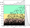 |
Fig. B.3 Mesh quality (as done in Fig. B.2) obtained via the successive barycentric subdivision of a triangle. |
Appendix B.2 Validation using the capacitance of different geometries
We test our implementation of the DSCD technique by computing the capacitance in vacuum of capacitors of different geometries, and comparing such capacitance with their expected value. In particular, we analyze the case of capacitors made of:
Two concentric spherical shells of radii R1 and R2. In this configuration, the capacitance is
![Mathematical equation: $\[C=\frac{4 \pi \varepsilon_{0}}{R_{1}^{-1}+R_{2}^{-1}}\]$](/articles/aa/full_html/2026/03/aa54409-25/aa54409-25-eq54.png) . The capacitor surfaces are closed in this configuration, meaning that the capacitance value C is exact.
. The capacitor surfaces are closed in this configuration, meaning that the capacitance value C is exact.Two parallel planar disks of radii R and separated by a distance d. In this configuration, we use the results of Reichert & Ristivojevic (2020), where approximations are given for the capacitance C in the limit of small and large d/R. The approximation of C take into consideration the edge effects that arise at the border of the disks.
Two thin parallel wires of radii r, length L and separated by a distance d. In this configuration, the capacitance is
![Mathematical equation: $\[C=\frac{\pi \varepsilon_{0} L}{\ln \left(d / 2 / r+\sqrt{d^{2} / 4 / r^{2}-1}\right)}\]$](/articles/aa/full_html/2026/03/aa54409-25/aa54409-25-eq55.png) . In this configuration, the capacitor surfaces are not closed and the approximation of C that we use does not take into account the edge effects. This means that we expect the approximation to not be exact, even if still reasonably correct.
. In this configuration, the capacitor surfaces are not closed and the approximation of C that we use does not take into account the edge effects. This means that we expect the approximation to not be exact, even if still reasonably correct.A thin wire of radius r and length L and a cylinder of radius R and length L, placed concentrically. In this configuration, the capacitance is
![Mathematical equation: $\[C=\frac{2 \pi \varepsilon_{0} L}{\ln (R / r)}\]$](/articles/aa/full_html/2026/03/aa54409-25/aa54409-25-eq56.png) . As discussed in the previous case, also in this configuration the edge effects are not taken into account in the approximation of C.
. As discussed in the previous case, also in this configuration the edge effects are not taken into account in the approximation of C.
The results of our calculations for the capacitance are presented in Figs. B.4, B.5, B.6, B.7. In all cases, the results from the DSCD calculation are in agreement with the expected value of C obtained from the analytical approximations. In the case of Figs. B.6, B.7, the approximation is less satisfactory due to the edge effects.
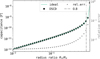 |
Fig. B.4 Capacitance of a concentric spherical capacitor (black dots) as a function of the radio of the radii of the two spherical shells, R1 and R2. The analytical exact result is presented as a green line, and the relative error between the numerical calculation and the exact result are the gray dots. |
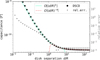 |
Fig. B.5 Same as Fig. B.4 but for a circular planar capacitor. The analytical approximations from Reichert & Ristivojevic (2020) are presented as green and red lines. |
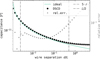 |
Fig. B.6 Same as Fig. B.4 but for a double this wire capacitor. The approximated result is presented as a green line. |
Appendix B.3 One example of validation: The antenna self-impedance
We validate the DSCD technique in the presence of an unmagnetized, Maxwellian plasma using the antenna self-impedance. This quantity is defined as the ratio of the voltage over current present on an electric antenna, in frequency space. We analyze here two case, both with a dipolar antenna composed of two electrodes. In one case, we use a double-wire antenna and in the other a double-sphere antenna.
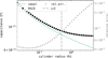 |
Fig. B.7 Same as Fig. B.4 but for a cylindrical and wire capacitor. The approximated result is presented as a green line. |
The self-impedance of an electric antenna is influenced by the presence of the surrounding plasma (Miyake 2009). This quantity can therefore be used for plasma diagnostic (see for example Blackwell et al. 2005 and Spencer et al. 2019). Even if the antenna impedance is not purposely measured, it is directly related to the noise that is measured passively due to the impact of electrons (Meyer-Vernet & Perche 1989). Therefore, knowledge of the antenna self-impedance is beneficial to antenna experiments that aim at characterizing space plasmas. We also note that the BepiColombo AM2P experiment is equipped to perform a self-impedance measurement.
We detail here two formulations of the antenna self-impedance. First, we start with a formulation that we call “EMF formulation.” In this case, the impedance is computed using the Electro-Motive-Force method combining the Maxwell and linearized Vlasov equations. We compute this quantity as presented in Meyer-Vernet & Perche (1989), and we present here the formulation for completeness’ sake:
![Mathematical equation: $\[Z_{e m f}=\frac{4 i}{\pi^2 \varepsilon_0 \omega} \int_0^{\infty} \frac{F(k)}{\varepsilon_L(k)} d k,\]$](/articles/aa/full_html/2026/03/aa54409-25/aa54409-25-eq57.png) (B.1)
(B.1)
where F(k) is the antenna response function and εL is the plasma longitudinal dielectric function. Second, we use the DSCD model to compute the antenna self-impedance, and we call this the “DSCD formulation.” To obtain this quantity, we impose a potential of +/- 1V on the two electrodes of the antenna. As a result of the DSCD model, we obtain the charge qm present on each of the antennas. We use the continuity equation to derive that
![Mathematical equation: $\[Z_{d s c d}=\frac{V}{I}=\frac{V}{i \omega q_m}.\]$](/articles/aa/full_html/2026/03/aa54409-25/aa54409-25-eq58.png) (B.2)
(B.2)
We compare the calculations of the antenna self-impedance using the “EMF formulation” and the “DSCD formulation” in Fig. B.8. We remark how the two provide very similar results, and therefore give an added validation to our numerical implementation of the DSCD technique.
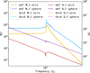 |
Fig. B.8 Antenna self-impedance (real and imaginary parts) for two antennas, one composed of two wire electrodes and the other of two spherical electrodes. Two techniques are used to compute the self-impedance: the “EMF formulation” and the “DSCD formulation,” both detailed in Appendix. B.3. |
Appendix C Monopolar approximation in DSCD
In this section we discuss the monopolar approximation used in the DSCD numerical model (Sect. 2.3) which leads to Eq. 4. We compute the electric potential of a charge distributed uniformly over a triangle, and compare it with the potential generated by the total charge concentrated (as a point-like charge) in the center of the triangle. We use as the center of the triangle its barycenter, meaning that for a triangle defined by its vertices (v1, v2, v3) the center is c = (v1 + v2 + v3)/3.
We generate a random triangle T, defined by its vertices (v1, v2, v3) with v1 = (0, 0, 0), v2 = (1, 0, 0), v3 = (l cos(θ), l sin(θ), 0) and where both l and θ are randomly generated with 0 < l < 1 and 0 < θ ≤ π/2. A total charge of 1 (normalized) is distributed on the triangle.
We compute the electric potential generated by such a triangle in two ways. First, we compute the potential generated as if all the charge is concentrated in the center c. This is the monopolar approximation, and is named Vmonopole. Second, we split the triangle using the same “wattx” approach described in Appendix A, and we sum the contribution of each of such triangles in order to compute an approximation of the potential generated by the triangular charge distribution. This result, which is not obtained in the monopolar approximation and is considered the “correct” one, is named Vint. The potential is computed in both ways in 3D space. In particular, between a distance of 1 and 10 from the center c of the triangle with 50 steps, and 50x50 angles in 3D space are used.
We compute the maximum normalized distance over all the investigated 3D space max.|Vmonopole − Vint.|/Vint.. We present this quantity as a histogram in Fig. C.1, as a function of the characteristic shape of the triangle (εX, εY) as defined in Appendix B.1. We note that as εY becomes smaller, the triangle becomes more “squished” and is less and less equilateral. Figure C.1 shows that smaller εY correspond to larger errors in the determination of the potential using the monopolar approximation. This reinforces the need, expressed in Appendix B.1, to construct the triangular mesh with triangles that lie in the upper part of Fig. C.1, shown in green in Fig. B.2 and Fig. B.3.
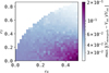 |
Fig. C.1 Maximum error (as defined in Sect. C) of the monopolar approximation for the electric potential generated by a triangular charge distribution. The axis εX and εY indicate the normalized shape of the triangle, as described in Sect. B.1 |
Appendix D Cross-validation of mutual impedance measurements in PEPSO
In this section we present the same mutual impedance measurement obtained using different instrumental setups. This is done in order to check the instrumental setup itself. We use three instruments: a HP4395 Network Analyzer, an Eclypse evaluation board with a Zynq7000 processor (Xilinx) which is equipped with Digital-to-Analog and Analog-to-Digital converters, a PicoScope 5000D oscilloscope. The Eclypse board and the associated software is the same used in Bucciantini et al. (2023) to provide mutual impedance measurements in a similar experimental setup. The schematic for the PicoScope measurement setup is presented in Fig. D.1.
We compare the measurements obtained by these instruments in Fig. D.2. In the case of the PicoScope measurements, we also compare the results with or without an added averaging of multiple measurements. The results of Fig. D.2 show that all the three instruments provide comparable results, validating the instrumental setup. We also present the plasma frequency measured by the Impedans Langmuir probe present inside the plasma chamber. The two lines correspond to a measurement of the electron density done before all the mutual impedance measurements and after. This is done in order to provide an indication of the variation of the plasma density during the course of all the measurements. As expected, the maximum in the mutual impedance spectrum is close to the measured plasma density, and in particular it is located at a slightly larger frequency, as expected (Sect. 4).
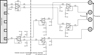 |
Fig. D.1 Circuit schematic for the mutual impedance experiment developed based on the PicoScope, using both its waveform generator (OUT) and oscilloscope (IN) capabilities. |
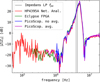 |
Fig. D.2 Comparison of mutual impedance measurements obtained using different instruments, as detailed in Appendix D. All the instruments provide comparable measurements. |
Appendix E Langmuir probe analysis
In this section we detail the analysis performed on the I-V sweeps provided by the Langmuir probe to obtain the plasma density and electron temperature independently from the mutual impedance experiment. We start by describing the Langmuir probe calibration routine performed in vacuum.
We first perform an I-V sweep in the plasma chamber under vacuum and in the absence of plasma. This measurement is presented in Fig. E.1 as a red line and is defined as a “vacuum non-biased” sweep. We remark that in this case, the measured current is around 3.12 μA, while we would expect a value compatible with zero, or at least of zero average over the sweep. This leak current is attributed to a combination of stray resistances present in the Langmuir probe setup. In order to mitigate this effect, we use a DC current compensation available in the Langmuir probe of −3.12 μA. The new I-V sweep obtained in vacuum is presented in Fig. E.1 as an orange line and is named “vacuum biased” sweep. The “vacuum biased” sweep is still not compatible with zero, and presents a resistive (linear) behavior. We average and interpolate a large (>50) number of I-V sweeps obtained in this way in order to construct a vacuum response curve that we define the “average vacuum biased” sweep.
One example of the measurements obtained in the presence of plasma is presented also in Fig. E.1. The I-V sweep obtained by the DC compensated probe is presented in blue, and is defined the “plasma biased” sweep. From this sweep, we subtract the “average vacuum biased” sweep, and with this we obtain the “plasma biased normalized” sweep, also shown in Fig. E.1 as a light blue line. This last “plasma biased normalized” sweep is the measurement we use for our analysis.
The analysis of the I-V sweep is performed following a multistep procedure (Lobbia & Beal 2017) shown in Fig. E.2. We start by identifying the potential at which the current is closest to zero, this is the probe’s floating potential Vfloating. We mark this potential as a vertical gray line in Fig. E.2. We then find the linear best fit with the I-V curve in the region that is defined by V < 0.9 · Vfloating and V < 0 V. This is the ion current, and is shown as a light red line in Fig. E.2. The ratio of Langmuir probe radius rLP over Debye length λDe is smaller than one rLP/λDe < 1 for all measurements we analyze. Thus, the approximation of an ion current varying linearly with the probe potential is validated (Jaeger et al. 1991; Laframboise 1966).
We compute the electron current Ie as the difference between the current measured during the I-V sweep and the linear interpolated ion’s current. We compute the derivative of this current, and present it as a light blue line in the middle panel of Fig. E.2. We smooth this derivative with a moving average (blue line in Fig. E.2), and find its maximum. The potential corresponding to the maximum is the plasma potential Vplasma, highlighted as a gray line in Fig. E.2. In the region between the floating and the plasma potential, we identify the electron retarding region, where we expect the I-V curve to follow approximately an exponential trend Ie ∝ eV/Te with Te measured in eV. We compute the linear best fit of the natural logarithm of the current as a function of the potential, shown in Fig. E.2 as green lines. The inverse of the slope of this line is the electron temperature. The electron density is obtained from the electron saturation current, that is defined as the electron current measured during the I-V sweep at the plasma potential Ie,sat. = Ie(Vplasma). This current satisfies the relation ![Mathematical equation: $\[I_{e, sat.} \simeq q_{e} n_{e} A_{L P} ~\sqrt{\frac{k_{B} T_{e}}{2 \pi m_{e}}}\]$](/articles/aa/full_html/2026/03/aa54409-25/aa54409-25-eq59.png) , and is therefore used to obtain the electron density using the measurement of the electron temperature obtained in the previous step. In the example presented in Fig. E.2ne = 3.6 · 105 cm−3.
, and is therefore used to obtain the electron density using the measurement of the electron temperature obtained in the previous step. In the example presented in Fig. E.2ne = 3.6 · 105 cm−3.
We remark that the ratio of Langmuir probe radius rLP over Debye length λDe is smaller than three rLP/λDe < 3 for all measurements we analyze. Thus, the approximation of an ion current varying linearly with the probe potential is valid (Lobbia & Beal 2017), meaning that the electron current can indeed be obtained from the total (measured) current minus the (fitted) ion current. It is then valid to obtain the plasma density and electron temperature from the analysis of the electron current.
We present an example of the measurements performed by the Langmuir probe while increasing the ionization current Ii. We show the dynamic spectrum of the “plasma biased normalized” Langmuir current as a function of Ii and the sweep voltage in Fig. E.3 in linear (top panel) and logarithmic (bottom panel) scale.
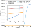 |
Fig. E.1 Vacuum calibration procedure used on the Langmuir probe described in Sect. 2.2. The different curves shown are detailed in Appendix E. |
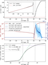 |
Fig. E.2 Analysis procedure employed on the I-V sweeps of the Langmuir probe in order to obtain a measurement of the plasma parameters. We describe in detail this analysis in Appendix E. |
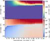 |
Fig. E.3 Dynamic spectrum of the Langmuir probe sweeps (“plasma biased normalized” measurements, as defined in Appendix. E), as a function of the plasma source ionization current, Ii. |
Appendix F Best-fit results for the mutual impedance experiment in a magnetized plasma
We present 12 representative examples of the best-fits between the mutual impedance measurements described in Sect. 3 (Fig. 8) and the modeled spectra using both a magnetized and unmagnetized instrument model, obtained using the procedure detailed in Sect. 4. Note that as the plasma density increases, the distance between the spectra obtained with the magnetized and unmagnetized models tends to decrease, as expected.
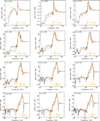 |
Fig. F.1 Examples of best-fit between PEPSO mutual impedance spectra (brown) and DSCD instrument model in the presence (resp. absence) of the magnetic field BEarth in orange (resp. green). Multiple modeled spectra are presented for different fpe/fce, from lighter to darker orange. Arrows indicate: the electron cyclotron frequency harmonics for f < fuh in yellow, the upper-hybrid frequency fuh in orange, the fqn frequencies for f > fuh in yellow. |
All Figures
|
Fig. 1 Left: schematic view of a mutual impedance emitting and receiving antenna. Middle: emission and reception signals measured by a typical mutual impedance experiment for five selected frequencies (in different colors). Right: mutual impedance measured for these five frequencies using the same colors, together with the mutual impedance spectrum measured for many frequencies in gray. |
| In the text | |
|
Fig. 2 Typical plasma parameters achievable in the plasma chamber. Panel a: plasma density and electron temperature. Panel b: associated plasma frequency and Debye length. The measurements are weighted according to their uncertainty: the brighter the color, the preciser the measurement. The electron cyclotron frequency associated with Earth’s magnetic field is shown as a vertical dashed gray line. |
| In the text | |
|
Fig. 3 Experimental relation between the measured plasma density, the electron temperature, and the ionization current Ii controlled on the plasma source. |
| In the text | |
|
Fig. 4 Measurements of the plasma density and electron temperature shown as a function of the time elapsed since the plasma source was turned on. The plasma stabilized with time, with a typical timescale of 30 minutes. |
| In the text | |
|
Fig. 5 Relation between the ionization current Ii and the discharge current Id measured in the plasma source of the plasma chamber. A total number of 146 245 measurements were used. |
| In the text | |
|
Fig. 6 Left: interior of the PEPSO plasma chamber, with the mutual impedance antennas (orange) and pre-amplifiers (yellow), the Langmuir probe (red), the plasma source (green), and the inlet for the vacuum pumps (violet). The Langmuir probe in the retracted position is hidden in the hole located on the right, at the support base. Right: three-dimensional mesh used to discretize the PEPSO plasma chamber in the DSCD mutual impedance numerical model. The pair of electrodes of the emitting (receiving) antenna are indicated as E1 and E2 (R1, R2). |
| In the text | |
|
Fig. 7 Hierarchy of our DSCD model. From left to right: DSCD model M, made of a collection of three-dimensional elements En. Each element is described by a triangular mesh composed of a number of triangles Tm. |
| In the text | |
|
Fig. 8 Two sets of measurements of mutual impedance spectra. The ionization current is on the horizontal axis, the frequency on the vertical axis, and we show the amplitude of the mutual impedance in color. Panels (a) and (b) (c and d): measurements taken with the antenna perpendicular (parallel) to the axis of the plasma chamber. Panel (a) and (c) (b and d) show measurements that were normalized to the mutual impedance in vacuum (to their maximum value, for illustration purposes). |
| In the text | |
|
Fig. 9 Representative set of magnetized mutual impedance amplitude spectra, normalized to vacuum, in the upper (lower) row with the antenna perpendicular (parallel) to the axis of the plasma chamber. The plasma density increases from left to right. The ionization filament current Ii is indicated in each panel, with the ratio of the plasma to electron cyclotron frequency fpe/fce. The following characteristic frequencies are shown as vertical lines: the harmonics of the electron cyclotron frequency, the upper hybrid frequency, and the series of fqn frequencies. |
| In the text | |
|
Fig. 10 Comparison results of the mutual impedance and Langmuir probe. Top: ratio of the plasma density |
| In the text | |
|
Fig. A.1 Subdivision of a triangle mesh element Tm used to compute the αm of Eq. A.1, using one of the three different techniques: “sing_int,” “gilet,” or “wattx.” |
| In the text | |
|
Fig. A.2 Left: Relative error obtained by the calculation of the αm parameter Eq. A.1 using different techniques. Right: Computation time for each technique. The histograms are computed using 5000 sample triangles, randomly generated. |
| In the text | |
|
Fig. B.1 Definition of the coordinates of the point (εX, εY) that is used to present the quality of the mesh triangles for the DSCD technique. |
| In the text | |
|
Fig. B.2 Mesh quality as defined in Appendix B for the numerical three-dimensional mesh used to describe the mutual impedance experiment inside the PEPSO plasma chamber, as presented in Fig. 6. |
| In the text | |
|
Fig. B.3 Mesh quality (as done in Fig. B.2) obtained via the successive barycentric subdivision of a triangle. |
| In the text | |
|
Fig. B.4 Capacitance of a concentric spherical capacitor (black dots) as a function of the radio of the radii of the two spherical shells, R1 and R2. The analytical exact result is presented as a green line, and the relative error between the numerical calculation and the exact result are the gray dots. |
| In the text | |
|
Fig. B.5 Same as Fig. B.4 but for a circular planar capacitor. The analytical approximations from Reichert & Ristivojevic (2020) are presented as green and red lines. |
| In the text | |
|
Fig. B.6 Same as Fig. B.4 but for a double this wire capacitor. The approximated result is presented as a green line. |
| In the text | |
|
Fig. B.7 Same as Fig. B.4 but for a cylindrical and wire capacitor. The approximated result is presented as a green line. |
| In the text | |
|
Fig. B.8 Antenna self-impedance (real and imaginary parts) for two antennas, one composed of two wire electrodes and the other of two spherical electrodes. Two techniques are used to compute the self-impedance: the “EMF formulation” and the “DSCD formulation,” both detailed in Appendix. B.3. |
| In the text | |
|
Fig. C.1 Maximum error (as defined in Sect. C) of the monopolar approximation for the electric potential generated by a triangular charge distribution. The axis εX and εY indicate the normalized shape of the triangle, as described in Sect. B.1 |
| In the text | |
|
Fig. D.1 Circuit schematic for the mutual impedance experiment developed based on the PicoScope, using both its waveform generator (OUT) and oscilloscope (IN) capabilities. |
| In the text | |
|
Fig. D.2 Comparison of mutual impedance measurements obtained using different instruments, as detailed in Appendix D. All the instruments provide comparable measurements. |
| In the text | |
|
Fig. E.1 Vacuum calibration procedure used on the Langmuir probe described in Sect. 2.2. The different curves shown are detailed in Appendix E. |
| In the text | |
|
Fig. E.2 Analysis procedure employed on the I-V sweeps of the Langmuir probe in order to obtain a measurement of the plasma parameters. We describe in detail this analysis in Appendix E. |
| In the text | |
|
Fig. E.3 Dynamic spectrum of the Langmuir probe sweeps (“plasma biased normalized” measurements, as defined in Appendix. E), as a function of the plasma source ionization current, Ii. |
| In the text | |
|
Fig. F.1 Examples of best-fit between PEPSO mutual impedance spectra (brown) and DSCD instrument model in the presence (resp. absence) of the magnetic field BEarth in orange (resp. green). Multiple modeled spectra are presented for different fpe/fce, from lighter to darker orange. Arrows indicate: the electron cyclotron frequency harmonics for f < fuh in yellow, the upper-hybrid frequency fuh in orange, the fqn frequencies for f > fuh in yellow. |
| In the text | |
Current usage metrics show cumulative count of Article Views (full-text article views including HTML views, PDF and ePub downloads, according to the available data) and Abstracts Views on Vision4Press platform.
Data correspond to usage on the plateform after 2015. The current usage metrics is available 48-96 hours after online publication and is updated daily on week days.
Initial download of the metrics may take a while.