| Issue |
A&A
Volume 707, March 2026
|
|
|---|---|---|
| Article Number | A226 | |
| Number of page(s) | 13 | |
| Section | Astronomical instrumentation | |
| DOI | https://doi.org/10.1051/0004-6361/202555106 | |
| Published online | 17 March 2026 | |
Euclid
VI. NISP-P optical ghosts
1
Max-Planck-Institut für Astronomie,
Königstuhl 17,
69117
Heidelberg,
Germany
2
CEA Saclay, DFR/IRFU, Service d’Astrophysique,
Bât. 709,
91191
Gif-sur-Yvette,
France
3
Leiden Observatory, Leiden University,
Einsteinweg 55,
2333 CC
Leiden,
The Netherlands
4
Université Paris-Saclay, CNRS, Institut d’astrophysique spatiale,
91405,
Orsay,
France
5
ESAC/ESA,
Camino Bajo del Castillo s/n., Urb. Villafranca del Castillo,
28692
Villanueva de la Cañada,
Madrid,
Spain
6
School of Mathematics and Physics, University of Surrey,
Guildford,
Surrey
GU2 7XH,
UK
7
INAF – Osservatorio Astronomico di Brera,
Via Brera 28,
20122
Milano,
Italy
8
IFPU, Institute for Fundamental Physics of the Universe,
via Beirut 2,
34151
Trieste,
Italy
9
INAF-Osservatorio Astronomico di Trieste,
Via G. B. Tiepolo 11,
34143
Trieste,
Italy
10
INFN, Sezione di Trieste,
Via Valerio 2,
34127
Trieste TS,
Italy
11
SISSA, International School for Advanced Studies,
Via Bonomea 265,
34136
Trieste TS,
Italy
12
Dipartimento di Fisica e Astronomia, Università di Bologna,
Via Gobetti 93/2,
40129
Bologna,
Italy
13
INAF-Osservatorio di Astrofisica e Scienza dello Spazio di Bologna,
Via Piero Gobetti 93/3,
40129
Bologna,
Italy
14
INFN – Sezione di Bologna,
Viale Berti Pichat 6/2,
40127
Bologna,
Italy
15
INAF – Osservatorio Astronomico di Padova,
Via dell’Osservatorio 5,
35122
Padova,
Italy
16
Space Science Data Center, Italian Space Agency,
via del Politecnico snc,
00133
Roma,
Italy
17
Dipartimento di Fisica, Università di Genova,
Via Dodecaneso 33,
16146,
Genova,
Italy
18
INFN – Sezione di Genova,
Via Dodecaneso 33,
16146
Genova,
Italy
19
Department of Physics “E. Pancini”, University Federico II,
Via Cinthia 6,
80126
Napoli,
Italy
20
INAF-Osservatorio Astronomico di Capodimonte,
Via Moiariello 16,
80131
Napoli,
Italy
21
Instituto de Astrofísica e Ciências do Espaço, Universidade do Porto, CAUP,
Rua das Estrelas,
4150-762
Porto,
Portugal
22
Faculdade de Ciências da Universidade do Porto,
Rua do Campo de Alegre,
4150-007
Porto,
Portugal
23
Dipartimento di Fisica, Università degli Studi di Torino,
Via P. Giuria 1,
10125
Torino,
Italy
24
INFN-Sezione di Torino,
Via P. Giuria 1,
10125
Torino,
Italy
25
INAF-Osservatorio Astrofisico di Torino,
Via Osservatorio 20,
10025
Pino Torinese (TO),
Italy
26
European Space Agency/ESTEC,
Keplerlaan 1,
2201 AZ
Noordwijk,
The Netherlands
27
Institute Lorentz, Leiden University,
Niels Bohrweg 2,
2333 CA
Leiden,
The Netherlands
28
Centro de Investigaciones Energéticas, Medioambientales y Tecnológicas (CIEMAT),
Avenida Complutense 40,
28040
Madrid,
Spain
29
Port d’Informació Científica, Campus UAB,
C. Albareda s/n,
08193
Bellaterra (Barcelona),
Spain
30
Institute for Theoretical Particle Physics and Cosmology (TTK), RWTH Aachen University,
52056
Aachen,
Germany
31
INAF – Osservatorio Astronomico di Roma,
Via Frascati 33,
00078
Monteporzio Catone,
Italy
32
INFN section of Naples,
Via Cinthia 6,
80126,
Napoli,
Italy
33
Institute for Astronomy, University of Hawaii,
2680 Woodlawn Drive,
Honolulu,
HI
96822,
USA
34
Dipartimento di Fisica e Astronomia “Augusto Righi” – Alma Mater Studiorum Università di Bologna,
Viale Berti Pichat 6/2,
40127
Bologna,
Italy
35
Instituto de Astrofísica de Canarias,
Vía Láctea,
38205
La Laguna, Tenerife,
Spain
36
Institute for Astronomy, University of Edinburgh, Royal Observatory,
Blackford Hill,
Edinburgh
EH9 3HJ,
UK
37
Jodrell Bank Centre for Astrophysics, Department of Physics and Astronomy, University of Manchester,
Oxford Road,
Manchester
M13 9PL,
UK
38
European Space Agency/ESRIN,
Largo Galileo Galilei 1,
00044
Frascati,
Roma,
Italy
39
Université Claude Bernard Lyon 1, CNRS/IN2P3, IP2I Lyon, UMR 5822,
Villeurbanne
69100,
France
40
Institute of Physics, Laboratory of Astrophysics, Ecole Polytechnique Fédérale de Lausanne (EPFL),
Observatoire de Sauverny,
1290
Versoix,
Switzerland
41
Institut de Ciències del Cosmos (ICCUB), Universitat de Barcelona (IEEC-UB),
Martí i Franquès 1,
08028
Barcelona,
Spain
42
Institució Catalana de Recerca i Estudis Avançats (ICREA),
Passeig de Lluís Companys 23,
08010
Barcelona,
Spain
43
UCB Lyon 1, CNRS/IN2P3, IUF, IP2I Lyon,
4 rue Enrico Fermi,
69622
Villeurbanne,
France
44
Departamento de Física, Faculdade de Ciências, Universidade de Lisboa,
Edifício C8, Campo Grande,
1749-016
Lisboa,
Portugal
45
Instituto de Astrofísica e Ciências do Espaço, Faculdade de Ciências, Universidade de Lisboa,
Campo Grande,
1749-016
Lisboa,
Portugal
46
Department of Astronomy, University of Geneva,
ch. d’Ecogia 16,
1290
Versoix,
Switzerland
47
INAF – Istituto di Astrofisica e Planetologia Spaziali,
via del Fosso del Cavaliere 100,
00100
Roma,
Italy
48
INFN – Padova,
Via Marzolo 8,
35131
Padova,
Italy
49
Aix-Marseille Université, CNRS/IN2P3, CPPM,
Marseille,
France
50
INFN – Bologna,
Via Irnerio 46,
40126
Bologna,
Italy
51
School of Physics, HH Wills Physics Laboratory, University of Bristol,
Tyndall Avenue,
Bristol
BS8 1TL,
UK
52
INAF – IASF Milano,
Via Alfonso Corti 12,
20133
Milano,
Italy
53
Universitäts-Sternwarte München, Fakultät für Physik, Ludwig-Maximilians-Universität München,
Scheinerstrasse 1,
81679
München,
Germany
54
Max Planck Institute for Extraterrestrial Physics,
Giessenbachstr. 1,
85748
Garching,
Germany
55
Dipartimento di Fisica “Aldo Pontremoli”, Università degli Studi di Milano,
Via Celoria 16,
20133
Milano,
Italy
56
INFN-Sezione di Milano,
Via Celoria 16,
20133
Milano,
Italy
57
Institute of Theoretical Astrophysics, University of Oslo,
PO Box 1029
Blindern,
0315
Oslo,
Norway
58
Jet Propulsion Laboratory, California Institute of Technology,
4800 Oak Grove Drive,
Pasadena,
CA
91109,
USA
59
Felix Hormuth Engineering,
Goethestr. 17,
69181
Leimen,
Germany
60
Technical University of Denmark,
Elektrovej 327,
2800
Kgs. Lyngby,
Denmark
61
Cosmic Dawn Center (DAWN),
Denmark
62
Institut d’Astrophysique de Paris, UMR 7095, CNRS, and Sorbonne Université,
98 bis boulevard Arago,
75014
Paris,
France
63
NASA Goddard Space Flight Center,
Greenbelt,
MD
20771,
USA
64
Department of Physics and Helsinki Institute of Physics,
Gustaf Hällströmin katu 2,
00014
University of Helsinki,
Finland
65
Université de Genève, Département de Physique Théorique and Centre for Astroparticle Physics,
24 quai Ernest-Ansermet,
CH-1211
Genève 4,
Switzerland
66
Department of Physics,
PO Box 64,
00014
University of Helsinki,
Finland
67
Helsinki Institute of Physics, Gustaf Hällströmin katu 2, University of Helsinki,
Helsinki,
Finland
68
Laboratoire détude de l’Univers et des phénoménes eXtrémes, Observatoire de Paris, Université PSL, Sorbonne Université, CNRS,
92190
Meudon,
France
69
Aix-Marseille Université, CNRS, CNES, LAM,
Marseille,
France
70
SKA Observatory, Jodrell Bank, Lower Withington, Macclesfield,
Cheshire
SK11 9FT,
UK
71
Centre de Calcul de l’IN2P3/CNRS,
21 avenue Pierre de Coubertin,
69627
Villeurbanne Cedex,
France
72
University of Applied Sciences and Arts of Northwestern Switzerland, School of Engineering,
5210
Windisch,
Switzerland
73
Universität Bonn, Argelander-Institut für Astronomie,
Auf dem Hügel 71,
53121
Bonn,
Germany
74
INFN-Sezione di Roma,
Piazzale Aldo Moro 2, c/o Dipartimento di Fisica, Edificio G. Marconi,
00185
Roma,
Italy
75
Dipartimento di Fisica e Astronomia “Augusto Righi” – Alma Mater Studiorum Università di Bologna,
via Piero Gobetti 93/2,
40129
Bologna,
Italy
76
Department of Physics, Institute for Computational Cosmology, Durham University,
South Road,
Durham
DH1 3LE,
UK
77
Université Paris Cité, CNRS, Astroparticule et Cosmologie,
75013
Paris,
France
78
CNRS-UCB International Research Laboratory, Centre Pierre Binetruy,
IRL2007,
CPB-IN2P3,
Berkeley,
USA
79
Aurora Technology for European Space Agency (ESA),
Camino bajo del Castillo s/n, Urbanizacion Villafranca del Castillo, Villanueva de la Cañada,
28692
Madrid,
Spain
80
Institut de Física d’Altes Energies (IFAE), The Barcelona Institute of Science and Technology,
Campus UAB,
08193
Bellaterra (Barcelona),
Spain
81
School of Mathematics, Statistics and Physics, Newcastle University,
Herschel Building,
Newcastle-upon-Tyne
NE1 7RU,
UK
82
DARK, Niels Bohr Institute, University of Copenhagen,
Jagtvej 155,
2200
Copenhagen,
Denmark
83
Waterloo Centre for Astrophysics, University of Waterloo,
Waterloo,
Ontario
N2L 3G1,
Canada
84
Department of Physics and Astronomy, University of Waterloo,
Waterloo,
Ontario
N2L 3G1,
Canada
85
Perimeter Institute for Theoretical Physics,
Waterloo,
Ontario
N2L 2Y5,
Canada
86
Université Paris-Saclay, Université Paris Cité, CEA, CNRS, AIM,
91191
Gif-sur-Yvette,
France
87
Centre National d’Etudes Spatiales – Centre spatial de Toulouse,
18 avenue Edouard Belin,
31401
Toulouse Cedex 9,
France
88
Institute of Space Science,
Str. Atomistilor, nr. 409 Măgurele,
Ilfov,
077125,
Romania
89
Consejo Superior de Investigaciones Cientificas,
Calle Serrano 117,
28006
Madrid,
Spain
90
Universidad de La Laguna, Departamento de Astrofísica,
38206
La Laguna, Tenerife,
Spain
91
Dipartimento di Fisica e Astronomia “G. Galilei”, Università di Padova,
Via Marzolo 8,
35131
Padova,
Italy
92
Institut für Theoretische Physik, University of Heidelberg,
Philosophenweg 16,
69120
Heidelberg,
Germany
93
Institut de Recherche en Astrophysique et Planétologie (IRAP), Université de Toulouse, CNRS, UPS, CNES,
14 Av. Edouard Belin,
31400
Toulouse,
France
94
Université St Joseph, Faculty of Sciences,
Beirut,
Lebanon
95
Departamento de Física, FCFM, Universidad de Chile,
Blanco Encalada
2008,
Santiago,
Chile
96
Universität Innsbruck, Institut für Astro- und Teilchenphysik,
Technikerstr. 25/8,
6020
Innsbruck,
Austria
97
Institut d’Estudis Espacials de Catalunya (IEEC), Edifici RDIT,
Campus UPC,
08860
Castelldefels, Barcelona,
Spain
98
Satlantis,
University Science Park, Sede Bld
48940,
Leioa-Bilbao,
Spain
99
Institute of Space Sciences (ICE, CSIC),
Campus UAB, Carrer de Can Magrans, s/n,
08193
Barcelona,
Spain
100
Instituto de Astrofísica e Ciências do Espaço, Faculdade de Ciências, Universidade de Lisboa,
Tapada da Ajuda,
1349-018
Lisboa,
Portugal
101
Cosmic Dawn Center (DAWN)
102
Niels Bohr Institute, University of Copenhagen,
Jagtvej 128,
2200
Copenhagen,
Denmark
103
Universidad Politécnica de Cartagena, Departamento de Electrónica y Tecnología de Computadoras,
Plaza del Hospital 1,
30202
Cartagena,
Spain
104
Kapteyn Astronomical Institute, University of Groningen,
PO Box 800,
9700 AV
Groningen,
The Netherlands
105
Infrared Processing and Analysis Center, California Institute of Technology,
Pasadena,
CA
91125,
USA
106
Dipartimento di Fisica e Scienze della Terra, Università degli Studi di Ferrara,
Via Giuseppe Saragat 1,
44122
Ferrara,
Italy
107
Istituto Nazionale di Fisica Nucleare, Sezione di Ferrara,
Via Giuseppe Saragat 1,
44122
Ferrara,
Italy
108
INAF, Istituto di Radioastronomia,
Via Piero Gobetti 101,
40129
Bologna,
Italy
109
Astronomical Observatory of the Autonomous Region of the Aosta Valley (OAVdA),
Loc. Lignan 39,
11020
Nus (Aosta Valley),
Italy
110
Department of Physics, Oxford University,
Keble Road,
Oxford
OX1 3RH,
UK
111
Department of Mathematics and Physics E. De Giorgi, University of Salento,
Via per Arnesano, CP-I93,
73100
Lecce,
Italy
112
INFN, Sezione di Lecce,
Via per Arnesano, CP-193,
73100
Lecce,
Italy
113
INAF – Sezione di Lecce, c/o Dipartimento Matematica e Fisica,
Via per Arnesano,
73100,
Lecce,
Italy
114
Institut d’Astrophysique de Paris,
98bis Boulevard Arago,
75014
Paris,
France
115
ICL, Junia, Université Catholique de Lille, LITL,
59000
Lille,
France
116
ICSC – Centro Nazionale di Ricerca in High Performance Computing, Big Data e Quantum Computing,
Via Magnanelli 2,
Bologna,
Italy
117
Instituto de Física Teórica UAM-CSIC,
Campus de Cantoblanco,
28049
Madrid,
Spain
118
CERCA/ISO, Department of Physics, Case Western Reserve University,
10900 Euclid Avenue,
Cleveland,
OH
44106,
USA
119
Technical University of Munich, TUM School of Natural Sciences, Physics Department,
James-Franck-Str. 1,
85748
Garching,
Germany
120
Max-Planck-Institut für Astrophysik,
Karl-Schwarzschild-Str. 1,
85748
Garching,
Germany
121
Laboratoire Univers et Théorie, Observatoire de Paris, Université PSL, Université Paris Cité, CNRS,
92190
Meudon,
France
122
Departamento de Física Fundamental. Universidad de Salamanca. Plaza de la Merced s/n,
37008
Salamanca,
Spain
123
Université de Strasbourg, CNRS, Observatoire astronomique de Strasbourg, UMR 7550,
67000
Strasbourg,
France
124
Center for Data-Driven Discovery, Kavli IPMU (WPI), UTIAS, The University of Tokyo,
Kashiwa,
Chiba
277-8583,
Japan
125
Dipartimento di Fisica – Sezione di Astronomia, Università di Trieste,
Via Tiepolo 11,
34131
Trieste,
Italy
126
California Institute of Technology,
1200 E California Blvd,
Pasadena,
CA
91125,
USA
127
Université Côte d’Azur, Observatoire de la Côte d’Azur, CNRS, Laboratoire Lagrange,
Bd de l’Observatoire,
CS 34229,
06304
Nice cedex 4,
France
128
University of California,
Los Angeles,
CA
90095-1562,
USA
129
Department of Physics & Astronomy, University of California Irvine,
Irvine
CA
92697,
USA
130
Departamento Física Aplicada, Universidad Politécnica de Cartagena,
Campus Muralla del Mar,
30202
Cartagena, Murcia,
Spain
131
Instituto de Física de Cantabria, Edificio Juan Jordá,
Avenida de los Castros,
39005
Santander,
Spain
132
Observatorio Nacional, Rua General Jose Cristino,
77-Bairro Imperial de Sao Cristovao,
Rio de Janeiro
20921-400,
Brazil
133
Institute of Cosmology and Gravitation, University of Portsmouth,
Portsmouth
PO1 3FX,
UK
134
Department of Computer Science, Aalto University,
PO Box 15400,
Espoo
00 076,
Finland
135
Instituto de Astrofísica de Canarias, c/ Via Lactea s/n, Departamento de Astrofísica de la Universidad de La Laguna,
Avda. Francisco Sanchez,
La Laguna
38200,
Spain
136
Caltech/IPAC,
1200 E. California Blvd.,
Pasadena,
CA
91125,
USA
137
Ruhr University Bochum, Faculty of Physics and Astronomy, Astronomical Institute (AIRUB), German Centre for Cosmological Lensing (GCCL),
44780
Bochum,
Germany
138
Department of Physics and Astronomy,
Vesilinnantie 5,
20014
University of Turku,
Finland
139
Serco for European Space Agency (ESA),
Camino bajo del Castillo s/n,
Urbanizacion Villafranca del Castillo, Villanueva de la Cañada,
28692
Madrid,
Spain
140
ARC Centre of Excellence for Dark Matter Particle Physics,
Melbourne,
Australia
141
Centre for Astrophysics & Supercomputing, Swinburne University of Technology,
Hawthorn,
Victoria
3122,
Australia
142
Department of Physics and Astronomy, University of the Western Cape,
Bellville,
Cape Town,
7535,
South Africa
143
DAMTP, Centre for Mathematical Sciences,
Wilberforce Road,
Cambridge
CB3 0WA,
UK
144
Kavli Institute for Cosmology Cambridge,
Madingley Road,
Cambridge,
CB3 0HA,
UK
145
Department of Astrophysics, University of Zurich,
Winterthurerstrasse 190,
8057
Zurich,
Switzerland
146
Department of Physics, Centre for Extragalactic Astronomy, Durham University,
South Road,
Durham,
DH1 3LE,
UK
147
IRFU, CEA, Université Paris-Saclay,
91191
Gif-sur-Yvette Cedex,
France
148
Oskar Klein Centre for Cosmoparticle Physics, Department of Physics, Stockholm University,
Stockholm
106 91,
Sweden
149
Astrophysics Group, Blackett Laboratory, Imperial College London,
London
SW7 2AZ,
UK
150
Univ. Grenoble Alpes, CNRS, Grenoble INP, LPSC-IN2P3,
53, Avenue des Martyrs,
38000
Grenoble,
France
151
INAF-Osservatorio Astrofisico di Arcetri,
Largo E. Fermi 5,
50125
Firenze,
Italy
152
Dipartimento di Fisica, Sapienza Università di Roma,
Piazzale Aldo Moro 2,
00185
Roma,
Italy
153
Centro de Astrofísica da Universidade do Porto,
Rua das Estrelas,
4150-762
Porto,
Portugal
154
HE Space for European Space Agency (ESA), Camino bajo del Castillo s/n, Urbanizacion Villafranca del Castillo,
Villanueva de la Cañada,
28692
Madrid,
Spain
155
Department of Astrophysical Sciences, Peyton Hall, Princeton University,
Princeton,
NJ
08544,
USA
156
INAF-Osservatorio Astronomico di Brera, Via Brera 28, 20122 Milano, Italy, and INFN-Sezione di Genova,
Via Dodecaneso 33,
16146,
Genova,
Italy
157
Theoretical astrophysics, Department of Physics and Astronomy, Uppsala University,
Box 515,
751 20
Uppsala,
Sweden
158
Mathematical Institute, University of Leiden,
Einsteinweg 55,
2333 CA
Leiden,
The Netherlands
159
ASTRON, the Netherlands Institute for Radio Astronomy,
Postbus 2,
7990 AA,
Dwingeloo,
The Netherlands
160
Anton Pannekoek Institute for Astronomy, University of Amsterdam,
Postbus 94249,
1090 GE
Amsterdam,
The Netherlands
161
Center for Advanced Interdisciplinary Research, Ss. Cyril and Methodius University in Skopje,
Macedonia
162
Institute of Astronomy, University of Cambridge,
Madingley Road,
Cambridge
CB3 0HA,
UK
163
Space physics and astronomy research unit, University of Oulu,
Pentti Kaiteran katu 1,
90014
Oulu,
Finland
164
Center for Computational Astrophysics, Flatiron Institute,
162 5th Avenue,
New York,
NY
10010,
USA
★ Corresponding author: This email address is being protected from spambots. You need JavaScript enabled to view it.
Received:
10
April
2025
Accepted:
18
July
2025
Abstract
The Near-Infrared Spectrometer and Photometer (NISP) on board Euclid includes several optical elements in its path that introduce artefacts into the data from non-nominal light paths. To ensure uncontaminated source photometry, these artefacts must be accurately accounted for. This paper focuses on two specific optical features in NISP’s photometric data (NISP-P): ghosts caused by the telescope’s dichroic beamsplitter, and the bandpass filters within the NISP fore-optics. Both ghost types exhibit a characteristic morphology and are offset from the originating stars. The offsets are well modelled using 2D polynomials; only stars brighter than approximately 10 magnitudes in each filter produce significant ghost contributions. The masking radii for these ghosts depend on both the source-star brightness and the filter wavelength, ranging from 20 to 40 pixels. We present the final relations and models used in the near-infrared (NIR) processing function (PF) to mask these ghosts for Euclid’s Quick Data Release (Q1).
Key words: instrumentation: photometers / space vehicles: instruments
© The Authors 2026
 Open Access article, published by EDP Sciences, under the terms of the Creative Commons Attribution License (https://creativecommons.org/licenses/by/4.0), which permits unrestricted use, distribution, and reproduction in any medium, provided the original work is properly cited.
This article is published in open access under the Subscribe to Open model.
Open Access funding provided by Max Planck Society.
1 Introduction
Euclid was launched in July 2023 and started its nominal observations, the Euclid Wide Survey (EWS), in February 2024. An overview of the mission, including early results from the Performance Verification (PV), is given in Euclid Collaboration: Mellier et al. (2025). Euclid’s two instruments, the optical imager VIS and the Near-Infrared Spectrometer and Photometer (NISP), are described in detail respectively in Euclid Collaboration: Cropper et al. (2025) and Euclid Collaboration: Jahnke et al. (2025). Both instruments can observe the sky simultaneously by means of a dichroic beamsplitter. The VIS optical path is purely reflective, whereas NISP implements the dichroic in transmission and carries three filters and four lenses in its fore-optics. For Euclid to achieve its demanding scientific goals, the accurate masking of unwanted optical features is essential for uncontaminated source photometry.
The NISP delivers photometry in three bands (YE, JE, HE) to an average 5σ point-source depth of about 24.4 (Euclid Collaboration: Jahnke et al. 2025) in the EWS. In Fig. 1, we show the nominal light path through the NISP optical elements. Although the optics of Euclid have a complex interference coating layout for passband-forming and optical optimisation, several parasitic reflections are still seen within the photometric (NISP-P) data. In this paper we describe and model the two most common parasitic reflections in detail, the NISP dichroic and filter ghosts.
The two features are caused by an internal double-reflection inside the respective optical element. The added optical path length – two times the traversed element thickness in combination with the respective refractive index – results in a defocused image of the ghosts on the focal plane array (FPA). The considerable oblique angles of incidence (AOIs) in Euclid’s telescopic off-axis design (Racca et al. 2016) are naturally responsible for the displacement of the dichroic ghosts from their source stars in the FPA (see Fig. 1; bottom). As these offsets are related to the incoming AOIs, we see variations across the FPA. We note here that VIS also has a dichroic ghost that is described in Euclid Collaboration: Cropper et al. (2025) and Euclid Collaboration: McCracken et al. (2026). However, the incoming AOIs are almost normal to the filter surface, so the displacement of the filter ghosts from their source stars arises mostly from the internal reflection off the spherically convex surface of the entrance side of the filter (Euclid Collaboration: Jahnke et al. 2025).
Other unwanted effects not discussed in detail in this paper include persistence arcs from the filter wheel, arc-like reflections from bright stars likely caused by the NISP lenses, and glints from out-of-field bright stars. Brief descriptions and examples are shown in Figs. 19–21 of Euclid Collaboration: Jahnke et al. (2025).
In Sect. 2, we describe the data used to characterise the dichroic and filter ghosts, while the detection algorithms are described in Sect. 3. We describe the characteristic of the dichroic and filter ghosts in Sects. 4 and 5, respectively. Finally, we conclude in Sect. 6. All magnitudes in this paper, unless stated otherwise, are in the AB system and all object magnitudes used for the ghost relations that are beyond the NISP saturation limit are transformed from Gaia as in Euclid Collaboration: Polenta et al. (2026). On-sky sizes in figures are reported using a pixel scale of 0.3″ pixel−1 (Euclid Collaboration: Jahnke et al. 2025).
2 Data
To model the NISP dichroic and filter ghosts, we looked at processed NISP-P data from PV, with the most current version of the near-infrared (NIR) processing function (PF) (see Euclid Collaboration: Polenta et al. 2026 for details) at the time of data extraction. In order to have bright stars in multiple positions on the detector to fully cover the FPA, we chose observations with a large number of widely dithered exposures. This includes (i) the self-calibration field (Euclid Collaboration: Mellier et al. 2025) near the north ecliptic pole consisting of 60 dithers within a 1◦ radius; (ii) observations of the Hubble Space Telescope CALSPEC white dwarf GRW+70 5824 (Bohlin et al. 2020) used for spectrophotometric calibration (Euclid Collaboration: Copin et al. 2026), placing the star at five positions on each detector; and (iii) the survey validation observations, which consisted of visits of multiple different fields, including the Chandra Deep Field South (CDFS; Giacconi et al. 2001), COSMOS (Scoville et al. 2007), the Euclid Deep Field North (EDF-N; Euclid Collaboration: Mellier et al. 2025), GOODS-N (Giavalisco et al. 2004), and the Euclid Deep Field South (EDF-S; Euclid Collaboration: Mellier et al. 2025).
This resulted in a total of 3270 images available for ghost detection, which contain 6023 instances where a suitably bright star falls onto the detectors.
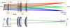 |
Fig. 1 <mono>Zemax</mono> ray tracing. Top panel: nominal light path through the NISP optical elements. We note that the dichroic is actually a part of the telescope and not of the NISP. The different colours show the light paths for three different sources in the field of view. For details of the optical layout and components (see Euclid Collaboration: Jahnke et al. 2025). Bottom panel: selecting the middle (green) rays of the top panel, we show how the light is internally reflected inside the dichroic to produce a ghost that is offset from the source position. A similar double reflection happens in the filter to produce the filter ghost (suppressed in this plot for clarity). |
3 Detection
During the NISP ground test campaign (which was performed on the NISP flight model, and thus excludes the dichroic; see Euclid Collaboration: Gillard et al. 2026 for full details), a number of tests were undertaken inside a vacuum chamber to verify NISP’s optical performance. One such test provided a rough estimate of filter ghost images within NISP. All measurements were compared with Zemax simulations to validate and clarify the output data from the NISP system. This included a model of the dichroic ghost to estimate the expected shape and offsets of the dichroic ghosts. The main purpose of these dichroic ghost simulations was to enable the inclusion of realistic dichroic ghosts in the NISP simulations and to prepare the processing pipelines for ghost masking. These simulations provided a good estimate for the dichroic ghost, but were not built to produce reliable models for direct comparison with real data.
Therefore, initial flight masking models for both the dichroic ghosts and the filter ghosts were manually rebuilt using a limited number of self-calibration observations. Initially, for each observation each of the 16 H2RG detectors was treated separately, and the position of the bright star along with the positions of the resulting dichroic and filter ghosts within the detector were recorded. The offsets between the position of the bright star in FPA coordinates (where the NISP pixel pitch is 18 µm in both direction; Euclid Collaboration: Jahnke et al. 2025) and the positions of the dichroic and filter ghosts were then used to build the initial 2D models to describe the ghost positions.
Next, a code to automatically find and determine the positions and other characteristics of the ghosts was used on all the available data. These characteristics were used to build a new ghost model. As better methods were developed and tested, this code was run multiple times, refining both the detection algorithm and the ghost model, which served as the initial guess for predicting ghost positions at each iteration. In this way, the model can be easily updated in the future once more data are available. As the model is built on FPA coordinates, it is independent of the detector positions and the gaps within the FPA footprint. Thus, the code was also updated to work on bright star and ghost pairs that span across different detectors. From the data, it was found that only brighter stars with YE, JE, HE <10 produce dichroic and filter ghosts of concern that must be masked out. Next, we describe the detection algorithm.
First, in order to find bright near-infrared stars in the footprint, for each observation, all stars with J2MASS,Vega < 8 and within 0.◦5 radius are queried from 2MASS (Skrutskie et al. 2006). For each star that falls onto a detector, the position of the star in pixel coordinates is determined using a 2D Gaussian centroid and is converted into FPA coordinates. Due to the saturated nature of these stars in the Euclid data, the final magnitudes were obtained by transforming their Gaia magnitudes to the Euclid system (to be consistent with the NIR PF, see Euclid Collaboration: Polenta et al. 2026). Then, using the initial guess for the ghost position, 60 × 60 pixel (80 × 80 pixel) cutouts are created for the dichroic (filter) ghost. A 2D background for the cutouts is calculated by interpolating over a low-resolution background map. This low-resolution background map is created from the median within 10 × 10 super pixels (resulting in 6 × 6 and 8 × 8 maps for the dichroic and filter ghost cutouts, respectively); then a 3 × 3 pixel sliding 2D median filter is applied to suppress local under- and overestimations. After background subtraction, astronomical sources with a minimum size of four pixels and with a signal exceeding a threshold based on the background root mean square (RMS) (×2 for the dichroic and ×18 for the filter ghosts) are subtracted from the data by replacing the pixel values with the median background subtracted value.
To determine the positions and radii of the ghosts, we first renormalise the cutouts using a 10%, 90% clipping to boost the contrast. We then perform edge detection using the Canny filter (Canny 1986) implemented in the <mono>skimage</mono> Python package (van der Walt et al. 2014). Afterwards, a circular Hough transformation (Illingworth & Kittler 1987) is used to detect circular shapes in the edge image. The final radius of the ghosts and the corresponding central position are extracted from the Hough transformation, and converted to FPA coordinates for use in determining the models.
Due to the relatively constant radius of the dichroic ghost (see Sect. 4), the circular Hough transformation easily extracts the correct radius when using an initial estimate of 15–36 pixels (see Fig. 2). The filter ghosts are different, though. The thin ring present in them is highly field-dependent in shape and size (see Sect. 5), and results in both an inner and outer radius in the Canny edge image. Therefore, the true radius of the filter ghosts are harder to automatically determine with a fixed radius range. To counter this, a Gaussian profile was fitted to the total radial profile of the filter ghost cutouts, excluding the central region containing the cusp (see Fig. 3). The mean of the fitted Gaussian then provided an estimate of the radius for each filter ghost. These radius measurements were then used to build a simple model of the filter-ghost radius as a function of FPA position and then reincorporated into the code to allow a dynamic range for the Hough transformation. The initial radius range for the filter ghost is thus from rmod − 10 to rmod + 5 pixels, where rmod is the estimated radius from the simple model.
Another complication arises from the non-circular (elliptical) shape of the filter ghost. Therefore, we use an ellipse Hough transformation (Xie & Ji 2002) to look for the ring. The results are then filtered by the minimum values (20 pixels) and maximum values (30 pixels for the minor axis and 35 pixels for major axis) seen for the radii, as well as by a ratio of 1.3 between the minor and major axis, before finding the highest peak determined from the edge image. While the offsets of the filter ghost do not depend on the wavelength, the shape and brightness are wavelength dependent. Therefore, each filter needs to be treated separately in this analysis. Only the more compact filter ghosts in the YE band data were easily detectable in an automatic way.
Thus, the offsets of the filter ghost were only measured for the YE band on the individual data, while the shape (radius and orientation) of each filter was found separately on the stacked data (see Sect. 5).
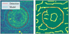 |
Fig. 2 Example of a dichroic ghost (left, 60 × 60 pixel – 18″ × 18″– cutout) and the automatic detection of the shape (red dashed line) based on edge detection using a circular Hough transformation (right). Also shown is the final model (cyan solid line) used for Q1 based on the detection values and the radius derived based on the magnitude of the source star (see Sect. 4). |
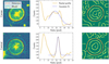 |
Fig. 3 Examples of filter ghosts near the FPA centre (bottom row) and near a corner (top row), highlighting the large field dependence. The left column shows an 80 × 80 pixel (24″ × 24″) cutout along with the automatic detection of the shape (red dashed line). Also shown is the final model (cyan solid line) used for Q1 based on the detection values, and the radius derived based on the magnitude of the source star (see Sect. 5). The middle column shows the total radial profile of the filter ghost cutout, and the Gaussian fit used as an initial guess for the detection radius. In the right column we display the edge image created from the Canny filter and the automatic detection of the shape (red dashed line) based on an elliptical Hough transformation. |
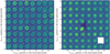 |
Fig. 4 Shape of the dichroic ghost (left panel) and filter ghost (right panel) as a function of field position. For the dichroic ghosts, the images are made from a median combination of 60 × 60 pixel (18″ × 18″) cutouts based on a 20-fold binning on the FPA, restricted to a single magnitude bin in HE band. For the filter ghosts, the images are made from a median combination of 80 × 80 pixel (24″ × 24″) cutouts on a 20-fold binning on the FPA, restricted to a single magnitude bin in the YE band. The number of cutouts used to create each median is given in the top right of each median cutout. For the blank square we could not find suitable stars within that region of the FPA. The artefacts, such as arcs, streaks, or circular residuals resulting from inadequate masking in the individual images, are caused by having data from few ghosts. |
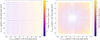 |
Fig. 5 Quiver plots showing the offset in millimetres from the source star to the dichroic (left) and filter ghost (right) across the FPA, i.e. −pOffset. The matrices used to describe these models are given in Appendices A and B. |
4 Dichroic ghost
Here we describe the general characteristics of the NISP-P dichroic ghost. The shape of the dichroic ghost is characterised by a doubled-ringed doughnut with an off-centre hole that is due to Euclid’s off-axis design. The general shape and size of the dichroic ghost changes very little as a function of FPA position (see Fig. 4; left).
4.1 Offsets
The offsets (defined as the difference between the centre of the circular fit determined for the dichroic ghost and the central position of the source star, in millimetres) on the YMOSA- and ZMOSA-axes for the dichroic ghost are both well described by third-order polynomials in the form of
 (1)
(1)
where pOffset provides the offset between the central positions of the dichroic ghost and the bright star pair in a given axis and ci,j is the matrix describing the coefficients of the polynomial for the offset in that axis. These matrices for the model used for Euclid’s first Quick Data Release (Q1) are given in Appendix A. As described in the Introduction, the displacement of the dichroic ghost on the FPA arises from the oblique AOIs from Euclid’s off-axis design. The total offset between the source star and the dichroic ghost is in the range 3–6 mm (167–335 pixels; see Fig. 5; left). The larger component on the YMOSA-axis is always positive when moving from the source star to the dichroic ghost position, while the offset in the ZMOSA-axis is smaller, but ranges from negative to positive. The RMS for the Q1 model is 0.082 mm (4.6 pixels).
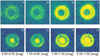 |
Fig. 6 Appearance of the dichroic ghost (top row) and filter ghost (bottom row) as a function of source-star brightness. For the dichroic ghosts, the images are made from a median combination of 60 × 60 pixel (18″ × 18″) cutouts, restricted to one region of the FPA for the HE band. For the filter ghosts, the images are made from a median combination of 80 × 80 pixel (24″ × 24″) cutouts, restricted to the central region of the FPA for the YE band. The number of cutouts used to create each median is given in the top right of each median cutout. |
4.2 Magnitude relations
Due to slight differences in the internal structure, the dichroic ghosts cannot be modelled and subtracted, and thus must be masked to avoid contamination of photometric measurements. To meet the top level requirement of a relative photometric error below 1.5% (Euclid Collaboration: Mellier et al. 2025), the detection-chain error must be smaller than 1% (Euclid Collaboration: Schirmer et. al. 2014). Using the error estimates from Euclid Collaboration: Schirmer et. al. (2014) and the targeted 5σ point-source depth in the EWS, it was calculated that this requirement equates to a maximum contribution from a ghost of 0.0866 e− pixel−1.
To determine the radius within which we need to mask the dichroic ghosts, Rmask, we need to determine at which radius its flux falls below the maximum contribution allowed from ghosts set by the requirement. Since the surface brightness of the dichroic ghost is dependent on the magnitude of the source star (see Fig. 6; top), as well as the wavelength it is observed in (see Fig. 7; top), each filter was treated separately while combining ghosts from source stars with similar magnitudes. For each dichroic ghost, we constructed 100 radial profiles starting from the centre position of the dichroic ghost and spread over the entire circumference to a radius of 50 pixels. A sigma-clipped median of these radial profiles was then calculated for multiple dichroic ghosts with similar source-star magnitudes to create a smooth radial profile. After subtracting any residual background, which was calculated from the median of the radial profile at a radius greater than 30 pixels, the radius at which the flux fell below the requirement was recorded. All measurements were then used to fit a power law, in the form of
 (2)
(2)
where R0 describes a radius in pixels and m the source-star magnitude. The coefficients found and used for Q1 are given in Table 1. The relation for each filter is shown in Fig. 8 (left). These relations were used to compute the radius of the dichroic-ghost mask based on the magnitude of the source star.
To determine the minimum brightness of a source star that would create a dichroic ghost that requires masking (mmin), we computed the surface brightness of the dichroic-ghost profiles calculated in the previous step. All flux within the previously calculated radius was included. A straight line was then fit to the mean flux per pixel in the dichroic ghost versus the flux from the source star. The magnitude of the source star at which the dichroic-ghost flux reached the requirement was then assigned as the mmin for the respective filter. The values used for Q1 are given in Table 1. These relations, as a function of source-star magnitude, are shown in Fig. 9 (left).
The NISP ground tests initially estimated the ratio of the peak flux in the source star to the peak surface brightness of filter ghosts to be 8 × 10⁻⁸. Using the NISP-P model PSF and zero points from Euclid Collaboration: Jahnke et al. (2025), we estimate the peak flux from the magnitude of the source star and find dichroic ghost ratios of 5.8 × 10⁻⁹, 5.7 × 10⁻⁹, and 8.3 × 10⁻⁹ for YE, JE, and HE respectively. These are an order of magnitude below the initial estimates, exceeding the predictions and highlighting the optical performance of NISP.
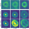 |
Fig. 7 Shape of the dichroic ghost (top row) and filter ghost (middle and bottom rows) as a function of waveband. For the dichroic ghosts, the images are made from a median combination of 60 × 60 pixel (18″ × 18″) cutouts, restricted to one region of the FPA and a single magnitude bin. For the filter ghosts, since there is a dependence of the shape on the FPA position, the images are made from a median combination of 80 × 80 pixel (24″ × 24″) cutouts, restricted to either the central region (middle) or a corner region (bottom) of the FPA and a single magnitude bin. The number of cutouts used to create each median is given in the top right of each median cutout. |
Q1 ghost masking parameters.
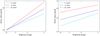 |
Fig. 8 Radius-magnitude relation, given by the coefficients in Table 1, for each filter for the dichroic ghost (left) and filter ghost (right; see Sects. 4.2 and 5.2). |
5 Filter ghost
Here we describe the general characteristics of the NISP-P filter ghost. The shape of the filter ghost varies greatly depending on the position on the FPA (see Fig. 4; right). The variations show a radially symmetric pattern, with the centre of the variations offset from the centre of the FPA at roughly YMOSA = −10 mm. The general shape consists of a thin ring and a central cusp. For small offsets from the pattern centre or off-centre FPA position, the ring is circular in shape and the cusp is point-like, while larger radial offsets result in the elongation of the ring and the central cusp. Along the central YMOSA- and ZMOSA-axis, the elongation of the ring is small while the central cusp changes into a four-point star-like shape with a radial axis and an axis perpendicular to the radial component. Towards the corners, the elongation is more pronounced, resulting in an oval shape, while the central cusp elongates much more in the plane perpendicular to the radial axis, thus becoming one-sided and resulting in a bird-shaped feature. These changes are the result of the geometric distortion introduced by the spherically convex surface of the entrance side of the filters. The curvature results in slightly different path lengths for the light during the second internal reflection, thus affecting the final image of the filter ghost. The size of the filter ghost and the sharpness of the ring and central cusp are also dependent on wavelength; the redder filters produce a more out-of-focus image (see Fig. 7; middle and bottom). This is due to the different filter thicknesses, which in turn result in slightly different path lengths, and thus focal points on the detector. Internal structures within the filter ghosts (multiple thin concentric rings) are seen only for the brightest stars up to YE, JE, HE > 4 (brighter stars are avoided by the survey, Euclid Collaboration: Mellier et al. 2025).
Spatial variation of the ratio of the major to minor axis of the filter ghost, which describes the elongation, is modelled by a second-order polynomial, pRadius in the same form as Eq. (1). The model shows the off-centre radially dependent pattern, where the filter ghost appears circular towards the centre of the pattern and more elongated, up to a ratio of 1.22, towards the corners (see Fig. 10; left). The orientation (in radians) of the elongation is also modelled by a second-order polynomial, pOrientation, of the same form. There is no rotational preference (set to 0) along the central axes, where the shape is more circular (see Fig. 10; right). Diagonal symmetry, i.e. between opposite corners, is seen with increasing negative rotation to the bottom left and increasing positive rotation towards the bottom right. The rotation is measured in radians from the YMOSA-axis in a clockwise direction, with a maximum of just over 1 radian (about 60◦) seen in both directions. The matrices containing the coefficients for these two models used for Q1 are given in Appendix B. The RMS for the ratio and orientation Q1 models is 0.23 and 0.63 radians respectively.
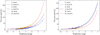 |
Fig. 9 Mean flux per pixel in the dichroic (left) and filter (right) ghost, calculated from the smoothed radial profiles as described in Sects. 4.2 and 5.2. The minimum brightness for masking is thus determined for each filter by the requirement that the ghost must contribute less than 0.0866 e− pixel−1. |
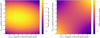 |
Fig. 10 Filter ghost shape and orientation. Left: model of the filter ghost’s major-to-minor axis ratio, i.e. the elongation. Right: model of the orientation of the filter ghost in radians, measured clockwise from the YMOSA-axis. The matrices used to describe these models are given in Appendix B. |
5.1 Offsets
The offsets (defined as the difference between the centre of the elliptical fit determined for the filter ghost and the central position of the source star, in millimetres) on the YMOSA- and ZMOSA-axes for the filter ghost are also both well described by third-order polynomials in the same form as Eq. (1). The matrices for the model used for Q1 are given in Appendix B. Similar to the shape variations, the offset for the filter ghost from the source star greatly varies across the FPA, ranging between 1 mm (56 pixels) and 17 mm (949 pixels), with the same off-centre radially symmetric pattern (see Fig. 5; right). Near the pattern centre–off-centre FPA position, the offset is as small as a few millimetres, while at greater radial positions the offsets are as large as 17 mm. The offset to the filter ghost from the source star is always positioned towards the pattern centre–off-centre FPA position. Again, these variations are due to the spherically convex surface of the entrance side of the filter. The curvature results in slightly different AOIs for the light during the second internal reflection, while the concave shape (as see from within the filter) results in the light path bending inwards, changing the offset of the filter ghost in a radially dependent way. The RMS for the Q1 model is 0.045 mm (2.5 pixels).
5.2 Magnitude relations
The surface brightness of the filter ghost is also dependent on the magnitude of the source star (see Fig. 6; bottom), and on the wavelength it is observed in (see Fig. 7; middle and bottom). Thus, to determine Rmask for the filter ghosts, we followed the same approach as done for the dichroic ghost described in Sect. 4.2; however, given that the radius and elongation of the filter ghosts depends not only on the wavelength, but also on the position on the FPA, only filter ghosts from the central region, where the shape is circular, are used to determine the radius-magnitude relation. The coefficients found and used for Q1 for Eq. (2) are given in Table 1. The relation for each filter is shown in Fig. 8 (right). These relations are used to compute the minor axis of the filter-ghost mask based on the magnitude of the source star. The major axis of the filter-ghost mask, which depends on the position on the FPA, is then obtained using the ratio model described in Sect. 5. The details on how this is done are described in Appendix B.
To determine mmin for the filter ghost we follow the same approach as done for the dichroic ghost described in Sect. 4.2, again restricting the calculation to the central regions where the filter ghost is circular in shape. The values used for Q1 are given in Table 1, with the data and fits shown in Fig. 9 (right).
Calculating the same ratios of source-star peak flux to ghost brightness for the filter ghosts as was done for the dichroic ghosts in Sect. 4.2, we find similar values for the filter ghost, with ratios of 1.3 × 10⁻⁸, 8.5 × 10⁻⁹, and 4.6 × 10⁻⁹ for YE, JE, and HE, respectively.
6 Discussion
As the data used to calculate these ghost models were from PV, they occurred before the first partial decontamination in March 2024. This decontamination was initiated after a noticeable throughput change, and resulted in two rounds of partial decontamination by warming up specific mirror surfaces during the subsequent period of heavy ice contamination between April and June 2024. An analysis of the dichroic ghost using data just before and after the March 2024 decontamination was performed as a sanity check to ensure no significant shifts in the ghost position occurred due to the decontamination, possibly due to changes in the alignment of the optics. No significant shifts between the data before and after the decontamination were found for the dichroic ghost. An analysis of the throughput of the dichroic and filter ghosts within NISP-P due to ice contamination was not conducted within the scope of this project and will be discussed elsewhere.
In this paper, we describe the characteristics and detection of the dichroic and filter ghosts in NISP-P images. For the detection, we developed an algorithm to automatically find and measure the positions of the dichroic and filter ghosts on NISP-P data. We presented the models used to describe the offsets, the radius, the shape, and the brightness of the dichroic and filters ghosts. The values found from selected PV data for the coefficients used in the models are given in Table 1, Appendices A and B.
From these data, we find a small range of offsets (3–6 mm or 167–335 pixels) for the dichroic ghosts, with a much larger range of 1–17 mm (56–949 pixels) for the filter ghosts. The shape of the dichroic ghosts is mostly circular and changes very little across the FPA or between filters. The radius of the circular dichroic-ghost mask ranges from 21 to 34 pixels based purely on the magnitude of the source star. The shape of the filter ghosts, however, depends greatly on their position on the FPA and on the filter of the observation. The shape is elliptical in nature, and thus requires an elliptical mask; the minor axis ranges from 23 to 45 pixels based on the magnitude of the source star, and the major axis up to 1.22 times greater than the minor axis depending on the position on the FPA. The surface brightness of both the dichroic and filter ghosts are roughly an order of magnitude below the initial exceptions from the NISP ground tests; where only stars with magnitudes <9–11 produce ghosts needing to be masked, which highlights the on-sky performance of NISP. On average, the dichroic ghosts are fainter than the filter ghosts in the same filter, but different relations between the surface brightness with respects to the wavelength are observed.
These models are used to mask affected pixels, where only ghosts resulting from stars are considered; while extended sources which are brighter than the magnitude limit and their respective ghosts are not considered, in the Q1 data release. While a description of how to use the matrices presented in this paper correctly, with examples using Python, is provided in Appendices A and B, the details of the ghost-masking routine within the NIR PF is described in Euclid Collaboration: Polenta et al. (2026). The further use of these masks during the stacking and catalogue creation is described in Euclid Collaboration: Romelli et al. (2026). For the Q1 data release, we find the total area lost due to masking of ghosts, persistence arcs, saturated stars, cosmic rays, dead pixels, and detector gaps is ∼4%. This percentage ranges between 2 and 10% over the Q1 footprint with varying stellar density. Even for the highest stellar density regions, this number falls below the error budget of 12% for area lost due to these effects in order for Euclid to comply with the science goals of the mission. As the survey continues, and more data become available, the models will be recomputed to update these parameters. However, we do not expect significant changes in the models over the lifetime of the mission resulting from optic shifts or ageing damage due to changes in the optics’ coatings. While the persistence arcs from the filter wheel are masked in the Q1 data (Euclid Collaboration: Polenta et al. 2026), further work to mask the other unwanted optical effects seen within the NISP-P data, such as the arc-like reflections from the NISP lenses and glints from out-of-field bright stars, is only planned for future data releases.
Acknowledgements
The authors at MPIA acknowledge funding by the German Space Agency DLR under grant number 50 QE 2303. We thank Pierre-Antoine Frugier for providing useful comments to improve the publication. The plots in this publication were prepared with <mono>Matplotlib</mono> (Hunter 2007). The Euclid Consortium acknowledges the European Space Agency and a number of agencies and institutes that have supported the development of Euclid, in particular the Agenzia Spaziale Italiana, the Austrian Forschungsförderungsgesellschaft funded through BMK, the Belgian Science Policy, the Canadian Euclid Consortium, the Deutsches Zentrum für Luft- und Raumfahrt, the DTU Space and the Niels Bohr Institute in Denmark, the French Centre National d’Etudes Spatiales, the Fundação para a Ciência e a Tecnologia, the Hungarian Academy of Sciences, the Ministerio de Ciencia, Innovación y Universidades, the National Aeronautics and Space Administration, the National Astronomical Observatory of Japan, the Netherlandse Onderzoekschool Voor Astronomie, the Norwegian Space Agency, the Research Council of Finland, the Romanian Space Agency, the State Secretariat for Education, Research, and Innovation (SERI) at the Swiss Space Office (SSO), and the United Kingdom Space Agency. A complete and detailed list is available on the Euclid web site (www.euclid-ec.org).
References
- Bohlin, R. C., Hubeny, I., & Rauch, T. 2020, AJ, 160, 21 [Google Scholar]
- Canny, J. 1986, IEEE Trans. Pattern Anal. Mach. Intell., PAMI-8, 679 [Google Scholar]
- Euclid Collaboration (Schirmer, M., et al.) 2014, Calibration Concept Document Part B (CalCD-B), Euclid Collaboration Document, EUCL-MPIA-RD-1-001 issue 3.1, 2014 September 1 [Google Scholar]
- Euclid Collaboration (Mellier, Y., et al.) 2025, A&A, 697, A1 [Google Scholar]
- Euclid Collaboration (Cropper, M. S., et al.) 2025, A&A, 697, A2 [Google Scholar]
- Euclid Collaboration (Jahnke, K., et al.) 2025, A&A, 697, A3 [Google Scholar]
- Euclid Collaboration (Copin, Y., et al.) 2026, A&A, in press, https://doi.org/10.1051/0004-6361/202554627 [Google Scholar]
- Euclid Collaboration (Gillard W., et al.) 2026, A&A, 707, A227 [Google Scholar]
- Euclid Collaboration (McCracken, H. J., et al.) 2026, A&A, in press, https://doi.org/10.1051/0004-6361/20255459 [Google Scholar]
- Euclid Collaboration (Polenta, G., et al.) 2026, A&A, in press, https://doi.org/10.1051/0004-6361/202554657 [Google Scholar]
- Euclid Collaboration (Romelli, E., et al.) 2026, A&A, in press, https://doi.org/10.1051/0004-6361/202554586 [Google Scholar]
- Giacconi, R., Rosati, P., Tozzi, P., et al. 2001, ApJ, 551, 624 [Google Scholar]
- Giavalisco, M., Ferguson, H. C., Koekemoer, A. M., et al. 2004, ApJ, 600, L93 [NASA ADS] [CrossRef] [Google Scholar]
- Hunter, J. D. 2007, Comput. Sci. Eng., 9, 90 [NASA ADS] [CrossRef] [Google Scholar]
- Illingworth, J., & Kittler, J. 1987, IEEE Trans. Pattern Anal. Mach. Intell., PAMI-9, 690 [Google Scholar]
- Racca, G. D., Laureijs, R., Stagnaro, L., et al. 2016, SPIE Conf. Ser., 9904, 99040O [NASA ADS] [Google Scholar]
- Scoville, N., Aussel, H., Brusa, M., et al. 2007, ApJS, 172, 1 [Google Scholar]
- Skrutskie, M. F., Cutri, R. M., Stiening, R., et al. 2006, AJ, 131, 1163 [NASA ADS] [CrossRef] [Google Scholar]
- van derWalt, S., Schönberger, J. L., Nunez-Iglesias, J., et al. 2014, PeerJ, 2, e453 [Google Scholar]
- Xie, Y., & Ji, Q. 2002, in 2002 International Conference on Pattern Recognition, 2, 957 [Google Scholar]
Appendix A Dichroic ghost
The third-order polynomials used to describe the dichroic ghost offsets (from the dichroic ghost position to the source-star position) are given by Eq. (1). The matrices containing the coefficients for the dichroic ghost offset in each axis, used for the Q1 models, are
 (A.1)
(A.1)
 (A.2)
(A.2)
 (A.3)
(A.3)
From these, the position of the dichroic ghost on the FPA (in millimetres) is given by
 (A.4)
(A.4)
The offsets themselves can be easily calculated in Python using the polyval2d function within numpy.polynomial.polynomial:
 (A.5)
(A.5)
Appendix B Filter ghost
Similarly, the third-order polynomials used to describe the filter ghost offsets (from the filter ghost position to the source-star position) are also given by Eq. (1), and can thus be calculated in the same way as the dichroic ghosts described in Appendix A. The matrices containing the coefficients for the filter ghost offset in each axis, used for the Q1 models, are
 (B.1)
(B.1)
 (B.2)
(B.2)
(B.3)
In addition to the offset, the ratio between the major and minor axis (i.e. the elongation) of the filter ghost, as well as the orientation of the ellipse describing the generic shape of the filter ghost also depends on the position on the FPA. The second-order polynomials used to describe these relations are also in the same form as Eq. (1), and can thus also be calculated using the same method in Python i.e. similarly to Eq. (A.5). The matrices containing the coefficients used to describe the elongation (radiusratio) and orientation relations, used for the Q1 models, are
 (B.4)
(B.4)
 (B.5)
(B.5)
The minor axis of the filter-ghost mask ( ) is described by Eq. (2), and is thus calculated the same way as the dichroic-ghost mask radius with the values given in Table 1. The major axis of the filter-ghost mask (using Python methods) is then calculated by
 (B.6)
(B.6)
while the orientation of  , moving clockwise from the YMOSA-axis in radians, is given by
 (B.7)
(B.7)
All Tables
All Figures
|
Fig. 1 <mono>Zemax</mono> ray tracing. Top panel: nominal light path through the NISP optical elements. We note that the dichroic is actually a part of the telescope and not of the NISP. The different colours show the light paths for three different sources in the field of view. For details of the optical layout and components (see Euclid Collaboration: Jahnke et al. 2025). Bottom panel: selecting the middle (green) rays of the top panel, we show how the light is internally reflected inside the dichroic to produce a ghost that is offset from the source position. A similar double reflection happens in the filter to produce the filter ghost (suppressed in this plot for clarity). |
| In the text | |
|
Fig. 2 Example of a dichroic ghost (left, 60 × 60 pixel – 18″ × 18″– cutout) and the automatic detection of the shape (red dashed line) based on edge detection using a circular Hough transformation (right). Also shown is the final model (cyan solid line) used for Q1 based on the detection values and the radius derived based on the magnitude of the source star (see Sect. 4). |
| In the text | |
|
Fig. 3 Examples of filter ghosts near the FPA centre (bottom row) and near a corner (top row), highlighting the large field dependence. The left column shows an 80 × 80 pixel (24″ × 24″) cutout along with the automatic detection of the shape (red dashed line). Also shown is the final model (cyan solid line) used for Q1 based on the detection values, and the radius derived based on the magnitude of the source star (see Sect. 5). The middle column shows the total radial profile of the filter ghost cutout, and the Gaussian fit used as an initial guess for the detection radius. In the right column we display the edge image created from the Canny filter and the automatic detection of the shape (red dashed line) based on an elliptical Hough transformation. |
| In the text | |
|
Fig. 4 Shape of the dichroic ghost (left panel) and filter ghost (right panel) as a function of field position. For the dichroic ghosts, the images are made from a median combination of 60 × 60 pixel (18″ × 18″) cutouts based on a 20-fold binning on the FPA, restricted to a single magnitude bin in HE band. For the filter ghosts, the images are made from a median combination of 80 × 80 pixel (24″ × 24″) cutouts on a 20-fold binning on the FPA, restricted to a single magnitude bin in the YE band. The number of cutouts used to create each median is given in the top right of each median cutout. For the blank square we could not find suitable stars within that region of the FPA. The artefacts, such as arcs, streaks, or circular residuals resulting from inadequate masking in the individual images, are caused by having data from few ghosts. |
| In the text | |
|
Fig. 5 Quiver plots showing the offset in millimetres from the source star to the dichroic (left) and filter ghost (right) across the FPA, i.e. −pOffset. The matrices used to describe these models are given in Appendices A and B. |
| In the text | |
|
Fig. 6 Appearance of the dichroic ghost (top row) and filter ghost (bottom row) as a function of source-star brightness. For the dichroic ghosts, the images are made from a median combination of 60 × 60 pixel (18″ × 18″) cutouts, restricted to one region of the FPA for the HE band. For the filter ghosts, the images are made from a median combination of 80 × 80 pixel (24″ × 24″) cutouts, restricted to the central region of the FPA for the YE band. The number of cutouts used to create each median is given in the top right of each median cutout. |
| In the text | |
|
Fig. 7 Shape of the dichroic ghost (top row) and filter ghost (middle and bottom rows) as a function of waveband. For the dichroic ghosts, the images are made from a median combination of 60 × 60 pixel (18″ × 18″) cutouts, restricted to one region of the FPA and a single magnitude bin. For the filter ghosts, since there is a dependence of the shape on the FPA position, the images are made from a median combination of 80 × 80 pixel (24″ × 24″) cutouts, restricted to either the central region (middle) or a corner region (bottom) of the FPA and a single magnitude bin. The number of cutouts used to create each median is given in the top right of each median cutout. |
| In the text | |
|
Fig. 8 Radius-magnitude relation, given by the coefficients in Table 1, for each filter for the dichroic ghost (left) and filter ghost (right; see Sects. 4.2 and 5.2). |
| In the text | |
|
Fig. 9 Mean flux per pixel in the dichroic (left) and filter (right) ghost, calculated from the smoothed radial profiles as described in Sects. 4.2 and 5.2. The minimum brightness for masking is thus determined for each filter by the requirement that the ghost must contribute less than 0.0866 e− pixel−1. |
| In the text | |
|
Fig. 10 Filter ghost shape and orientation. Left: model of the filter ghost’s major-to-minor axis ratio, i.e. the elongation. Right: model of the orientation of the filter ghost in radians, measured clockwise from the YMOSA-axis. The matrices used to describe these models are given in Appendix B. |
| In the text | |
Current usage metrics show cumulative count of Article Views (full-text article views including HTML views, PDF and ePub downloads, according to the available data) and Abstracts Views on Vision4Press platform.
Data correspond to usage on the plateform after 2015. The current usage metrics is available 48-96 hours after online publication and is updated daily on week days.
Initial download of the metrics may take a while.