| Issue |
A&A
Volume 707, March 2026
|
|
|---|---|---|
| Article Number | A138 | |
| Number of page(s) | 8 | |
| Section | Galactic structure, stellar clusters and populations | |
| DOI | https://doi.org/10.1051/0004-6361/202555637 | |
| Published online | 11 March 2026 | |
CAPOS: The bulge Cluster APOgee Survey
X. Chemical analysis of the Bulge Globular Cluster Djorg 2
1
Departamento de Astronomía, Universidad de Concepción,
Casilla 160-C,
Concepción,
Chile
2
Universidad Andres Bello, Facultad de Ciencias Exactas, Departamento de Física y Astronomía – Instituto de Astrofísica,
Autopista Concepcion-Talcahuano 7100,
Talcahuano,
Chile
3
Departamento de Astronomía, Facultad de Ciencias, Universidad de La Serena,
Av. Raul Bitran 1305,
La Serena,
Chile
4
Instituto de Astronomía, Universidad Católica del Norte,
Av. Angamos 0610,
Antofagasta,
Chile
★ Corresponding authors: This email address is being protected from spambots. You need JavaScript enabled to view it.
; This email address is being protected from spambots. You need JavaScript enabled to view it.
Received:
23
May
2025
Accepted:
1
December
2025
Abstract
Context. This study presents detailed elemental abundances in the intermediate-metallicity bulge globular cluster Djorg 2 based on high-resolution near-infrared spectra of six (R ~ 22 500) members obtained through the bulge Cluster APOgee Survey (CAPOS). CAPOS is focused on the study of clusters within the Galactic bulge and uses the APOGEE-2S as part of the Sloan Digital Sky Survey IV (SDSS-IV).
Aims. This study was undertaken to chemically explore this poorly studied cluster and to analyze it for the first time using the code BACCHUS, with the main objective of deriving the mean chemical abundances for a number of species and investigating the occurrence of multiple populations.
Methods. We employed BACCHUS to provide the line-by-line elemental abundances of a variety of species, including α-elements (O, Mg, Si, Ca, and Ti), light elements (C and N), the odd-Z element Al, the s-process element (Ce), and iron-peak elements (Fe and Ni).
Results. We found an average metallicity of [Fe/H] = –1.04 ± 0.06, without an indication of an intrinsic spread. The mean values for the other elements and their standard deviations are [C/Fe] = –0.35 ± 0.18, [N/Fe] = 0.38 ± 0.40, [O/Fe] = 0.22 ± 0.18, [Mg/Fe] = 0.38 ± 0.05, [Al/Fe] = 0.32 ±0.15, [Ca/Fe] = 0.21 ± 0.10, [Si/Fe] = 0.38 ± 0.05, [Ce/Fe] = +0.00 ± 0.06, [Ti/Fe] = +0.12 ± 0.08 and [Ni/Fe] = +0.09 ± 0.06.
Conclusions. The typical α-element enrichment in Djorg2 follows the trend of other metal-rich globular clusters. We found evidence for intrinsic spreads in C, N and O, which furthermore show the C:N and N:O anticorrelations that are typical of globular clusters. Ce shows no intrinsic variation, and in particular no correlation with N or Al. We found that Djorg 2 moves in a very elongated and flat orbit, that always remains inside the bulge and does not move far away in altitude above the Galactic plane. Moreover, it moves in a retrograde direction (backward to the rotation of the galaxy) and is not trapped by the galactic bar.
Key words: stars: abundances / stars: chemically peculiar / Galaxy: bulge / globular clusters: general / globular clusters: individual: Djorg 2
© The Authors 2026
 Open Access article, published by EDP Sciences, under the terms of the Creative Commons Attribution License (https://creativecommons.org/licenses/by/4.0), which permits unrestricted use, distribution, and reproduction in any medium, provided the original work is properly cited.
This article is published in open access under the Subscribe to Open model. This email address is being protected from spambots. You need JavaScript enabled to view it. to support open access publication.
1 Introduction
Globular clusters (GCs) serve as cosmic laboratories that enable the exploration of star formation and evolution within the Milky Way. As some of the oldest structures in the Galaxy, they provide critical insights into the timescales and conditions under which the Milky Way was assembled (see Massari et al. 2019; VandenBerg et al. 2013). Growing evidence of the chemical diversity and complexity of these systems has made the study of multiple stellar populations a key topic in understanding their evolutionary history. The formation models of the Milky Way and the study of its GC system are closely linked, because these models impose constraints on the properties of individual stars within these clusters (Muratov & Gnedin 2010; Renaud et al. 2016). In this context, the GC Djorg 2 represents an important case study for this purpose. A detailed study of its chemistry and orbit can provide new perspectives on nucleosynthesis and galactic evolution. It is particularly challenging to investigate GCs in the inner Galaxy ibecause the extinction os high and they can be confused with field stars from the Galactic bulge, thin and thick disks, and halo along the line of sight (Koch et al. 2016). As a result, the population of GCs in the Galactic bulge remains largely understudied and incomplete (e.g. Bica et al. 2016). Efforts have been made to obtain deep and homogeneous color-magnitude diagrams (CMDs) for bulge GCs (Minniti et al. 2017; Kerber et al. 2019; Saracino et al. 2019), while recent spectroscopic surveys of GC stars have provided valuable data (Vásquez et al. 2018). These studies have helped us to refine our knowledge of the distances, chemical compositions, and kinematics of bulge GCs. The GC population in the Galactic bulge is highly diverse and includes the most metal-rich clusters in the Milky Way. Interestingly, the metallicity of a considerable number of these clusters is about [Fe/H] ~ −1.0 dex (Pérez-Villegas et al. 2019; Bica et al. 2024) (Geisler et. al. in prep), and most of them display a blue horizontal branch (Bica et al. (2016); Cohen et al. (2018)). These clusters and their counterpart bulge stars (Savino et al. 2020) are likely among the oldest objects in the Galaxy (Barbuy et al. (2014), Barbuy et al. (2018)). This is supported by the well-established trend according to which older or more metal-poor clusters tend to exhibit bluer horizontal branches (e.g., Fig. 11 in Dias et al. 2016). Consequently, the presence of metal-rich clusters with a blue horizontal branch can only be attributed to an ancient formation age.
Recent investigations have demonstrated that many GCs host multiple stellar populations, each with a distinct metallicity and chemical composition characteristics. These phenomena are particularly evident in clusters such as NGC 2298, where the Mg–Al anticorrelation has been attributed to mixing and contamination processes by stars in different evolutionary stages. In this paper, we present H-band spectroscopy for six members of Djorg 2, using spectra from the bulge Cluster APOgee Survey (CAPOS, Geisler et al. (2021)), a contributed program of the Apache Point Observatory Galactic Evolution Experimental II survey (APOGEE-2, Majewski et al. (2017)) and the Sloan Digital Sky IV survey (Blanton et al. 2017; Ahumada et al. 2020). These spectra make it possible to derive detailed elemental abundances for a number of giant stars, and to achieve RVs with a precision better than 0.1 km s−1. This work focuses on exploring the stellar chemistry of Djorg 2, in particular, on the characterization of its multiple populations and the interpretation of the elemental abundances. Through a detailed analysis, our aim is to improve our understanding of the evolution of GCs and their effect on the chemical history of the Milky Way. By comparing Djorg 2 with other GCs, this study aims to identify patterns and trends that contribute to a coherent model of galactic evolution by providing valuable information about the conditions under which the cluster formed.
This paper is organized as follows. Section 2 presents an overview of the CAPOS data we analyzed toward Djorg 2. Section 3 presents our observations and data. Section 4 describes the atmospheric parameters .Section 5 describes our abundance analysis using the code BACCHUS. Our conclusions are presented in Section 6. In Section 7, we analyze the orbit of Djorg 2. We discuss our abundances and compare them with the literature in Section 8.
2 Djorg 2
Djorg 2 is a GC located toward the Galactic bulge at (l, b) = (+2.77°, −2.50°). Harris (2010) listed its metallicity as −0.65 and the reddening as 0.94. The cluster is located at a heliocentric distance of 8.75 ± 0.12 kpc, as derived by Ortolani et al. (2019).
Using enhanced imaging techniques available at the time, Djorgovski (1987) identified ESO 456-SC38 as a heavily obscured GC, which is also known as Djorgovski 2 (or Djorg 2). The first color-magnitude diagram (CMD) of the cluster in optical bands was provided by Ortolani et al. (1997), who determined that the cluster is located on the near side of the Galaxy. Furthermore, its red giant branch suggested a metal-rich nature with [Fe/H] −0.5. Subsequent infrared photometry by Valenti et al. (2010) yielded comparable results. The authors estimated a metallicity of [Fe/H] = –0.65 dex and a distance modulus of (m − M)0 = 14.23 mag. The most detailed available CMD is based on Hubble Space Telescope (HST) photometry (Ortolani et al. 2019) and Very Large Telescope (VLT), which refined these estimates, and reports [Fe/H] =–1.11 dex, a distance modulus of (m − M)0 = 14.71 ± 0.03 mag, and an age of 12.7 ±0.7 Gyr, with a blue horizontal branch.
Spectroscopic data for this cluster have only recently been acquired, and previous analyses have been based on a limited number of confirmed cluster members (Dias et al. (2016)), using four member stars, reported a radial velocity of −150 ± 28 km s−1, a metallicity of [Fe/H] = −0.79 ± 0.09 dex, and [Mg/Fe] = 0.28 ± 0.10 dex. Vásquez et al. (2018) analyzed three member stars and determined a radial velocity of −159.9 ± 0.5 km s−1 and a metallicity ranging from [Fe/H] −0.97 to −1.09 dex, depending on the adopted calcium triplet calibration (CaT). González-Díaz et al. (2023) also used CaT spectra of two members and derived a metallicity of –0.67 ± 0.10.
This cluster was observed as part of CAPOS, which was specifically designed to study the chemical history of clusters in the Galactic bulge (Geisler et al. 2021). Observations focused on red giant stars and obtained high-resolution spectra with an S/N suitable for the detailed analysis of Fe, α-element and proton-capture element abundances, such as Mg, Si, and Al. APOGEE data on this cluster were obtained as part of the CAPOS project (Geisler et al. 2021). They observed seven members and derived a mean metallicity of –1.07 ± 0.09 from the ASPCAP APOGEE pipeline and the release of DR16, and they corrected the ASPCAP values of stars with high N abundances for a small metallicity offset. Kunder & Butler (2020) used the same data but without the correction to derive a very similar mean. Most recently, Geisler et al, (2025) used ASPCAP and DR17 for six members and found –1.14 ±0.04 using a similar metallicity correction. They also found that the average [Si/Fe] abundance is +0.24 ±0.03 and reported a mean radial velocity of –151.9 ± 1.2 km/s.
3 Observations
We used data obtained through the Apache Point Observatory Galactic Evolution Experiment (APOGEE-2; Majewski et al. 2017) spectrograph, which observed ~657 135 stars as part of the SDSS-IV survey (Blanton et al. (2017)). APOGEE-2 operate in the near-infrared (NIR) with an H-band spectral resolution of R ~ 22 500 through using the 2.5 m Sloan Digital Sky Survey (SDSS) telescope (Gunn et al. 2006), which is located at the Las Campanas Observatory, Chile. APOGEE-2 has proved to be a key instrument for obtaining high-resolution spectra, which is particularly useful for precise chemical abundance determinations in giant stars typical of GC. The data we processed are part of the CAPOS program, which is aimed at studying GC in the bulge (Geisler et al. (2021)). The observations of the GCs were carried out during several observational campaigns, and red giant stars were selected as the primary candidates for a detailed spectroscopic analysis. The stars were identified and selected based on available photometry and precise positional data within the clusters (see Geisler et al. (2021) for details). These observations enabled the acquisition of spectra with a high signal-to-noise ratio (S/N > 100) that are adequate for a precise chemical analysis and precise determinations of the elemental abundance. The data were processed using the standard APOGEE pipeline, which includes initial reduction, atmospheric corrections, and spectral calibration. ASPCAP also derives radial velocities with an internal precision of ~0.1 km s−1 (Nidever et al. 2015). We used the final version of the APOGEE- 2 catalog published in December 2021 as part of the Data Release 17 of the Sloan Digital Sky Survey (SDSS), which is available in the SDSS IV science archive server.
Table 1 provides the APOGEE-2 designations, celestial coordinates, atmospheric parameters (see next section), radial velocity, S/N, Gaia DR3 and 2MASS magnitudes, and Gaia DR3 proper motions of the analyzed stars. These selections led to the previously mentioned total of six targets that were observed as part of the CAPOS survey (Geisler et al. 2021).
Fig. 1 (top left panel) shows the spatial distribution of the APOGEE DR17 stars toward the Djorg 2 field. Member stars were first selected to lie within the tidal radius (as shown in the figure). Next, members were limited to stars with Gaia DR3 PMs within 0.5 mas/yr of the cluster center as determined by Vasiliev & Baumgardt (2021). Next, we selected stars within two standard deviations of the mean cluster RV derived by Vasiliev & Baumgardt (2021), and stars within 3 σ of their mean cluster metallicity. Finally, we verified that all our final members are located along the main RGB of the cluster. Proper motions (PMs); μα cos(δ) = 0.54 and μδ = −3.04 (Geisler et al. 2021). The bottom left panel in Fig. 1 presents the updated version of the PMs using Gaia DR3, and the top right panel presents DR17 iron content versus radial velocities. We find a mean radial velocity of RV=–149.8 km/s. Finally, bottom and PM-based cluster members.
The targets are located within the tidal radius of the cluster and also exhibit similar PMs, agree with the same evolutionary sequence in the optical and NIR CMDs, and have comparable RV and metallicities. These factors indicate that the six CAPOS stars are highly probable cluster members.
Main physical parameters of Djorg 2.
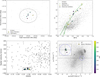 |
Fig. 1 Global properties of the Djorg 2 targets. In all the panels, our targets are represented using a star-symbol. Top left panel: spatial position. The color-coded symbols represent the S/R of the stars (labeled in bottom left panel) with APOGEE spectra. Other APOGEE targets in the field are shown as gray dots. A circle with the tidal radius (Harris 2010) is overplotted. Bottom-left panel: radial velocity vs. metallicity of our members compared to field stars. The black box encloses the cluster members within 0.2 dex and 15 km/s from the nominal mean [Fe/H]=–1.04 dex and RV=–149.8 km/s, as determined in this work. Top-right panel: color–magnitude diagram corrected for differential reddening in the Gaia Bp and 2MASS K bands within 5’. Our targets all lie along the red giant branch. The best isochrone fit is represented by green circles. Field stars are plotted as gray dots. Bottom-right panel: proper motion density distribution of stars located within the tidal radius from the cluster center. The inner plot in the top left corner shows a zoom-in of the cluster squared in 0.7 × 0.7 mas yr−1 and enclosed in a proper motion radius of 0.5 mas yr−1, shown as a blue circle. The dashed gray lines are centered on the cluster center PM values and PM-based cluster members are indicated as yellow circles. |
4 Atmospheric parameters
The CMD presented in Figure 1 was corrected for differential reddening using the same method as employed by Romero- Colmenares et al. (2021) and Fernández-Trincado et al. (2022). For this purpose, we selected all RGB stars within a radius of 5 arcmin from the cluster center whose proper motions were compatible with the mean value of the cluster. First, we drew a ridge line along the RGB and calculated the distance from this line along the reddening vector for each of the selected RGB stars. The vertical projection of this distance gives the differential interstellar absorption AK at the position of the star, and the horizontal position gives the differential optical+NIR reddening E(BP-K) at the position of the star. After this first step, we selected the three nearest RGB stars for each star of the field, calculated the mean differential interstellar absorption AK and the mean differential optical+NIR reddening E(BP–K), and finally subtracted these mean values from its BP–K optical+NIR colors and K magnitudes. We emphasize that the number of reference stars used for the reddening correction is a compromise between a correction that is affected as little as possible by photometric random error and the highest possible spatial resolution.
In order to estimate the parameters of the cluster, we performed an isochrone fitting of the RGB using the PARSEC database (Bressan et al. 2012). The extinction laws of Cardelli et al. (1989) and O'Donnell (1994) were used. The free parameters for this fitting were the true distance modulus, (m-M)0 (or the equivalent distance in pc), the interstellar absorption in the V band, AV, and the reddening-law coefficient, RV. These three parameters were estimated simultaneously using the BP-K versus K, BP–RP versus G and J–K versus K CMDs, assuming an age of 12 Gyr and a global metallicity [M/H] that considered the α-enhancement of the cluster according to the relation by Salaris et al. (1993). [Fe/H] was obtained from Harris (2010) and [α/Fe] was assumed to be +0.4. [M/H] was then adjusted during the fitting procedure in order to match the shape of the upper RGB.
The coefficient of the extinction law RV is usually assumed to be 3.1 but can vary significantly from the canonical value, especially in the direction of the Galactic bulge (Nataf et al. 2016), where it can easily take lower values. We found an extinction law coefficient RV = 2.30 ± 0.1. Moreover, we achieved a fit for the distance d⊙ = 11300 kpc that is, (m-M)0=15.27 ± 0.05, and an interstellar absorption AV = 2.36 ± 0.05. Finally, the interstellar absorption and the extinction-law coefficient we found can be translated into E(B-V)= 1.03, which is somewhat higher than the foreground interstellar reddening given by Harris (2010), that is, E(B-V)=0.94. This discrepancy is very likely due to the higher RV used in previous studies.
The method we applied to obtain Teff and log g from photometry was the same as that of Fernández-Trincado et al. (2022). We used the differentially corrected BP–K versus K CMD of Figure 4 and projected the position of each target horizontally until it intersected the RGB of the best-fitting isochrone.
We then assumed the Teff and log g of each target to be the temperature and gravity of the point of the isochrone with the same Ks magnitude as the star, interpolating if necessary. We underline the fact that for highly reddened objects such as Djorg 2, the absorption correction to be applied to each point of the isochrone during the fitting process depends on its temperature. We took this effect into account by calculating for each point of the isochrone and each photometric filter (G, BP, RP, J, H and K), the effective wavelength to be input in the Cardelli et al. (1989) and O'Donnell (1994) extinction law. Without this procedure, it is not possible to obtain a reliable fit of the RGB, especially of the upper and cooler part. Finally, with Teff and log g fixed, we employed the relation from Mott et al. (2020) for FGK stars to determine the microturbulence parameter ξt. The stellar parameters are listed in Table 1.
5 Abundance determination
The method of deriving stellar abundances is the same as was described by Fernández-Trincado et al. (2022). For this purpose, we made use of the code called Brussels Automatic Code for Characterizing Accuracy (BACCHUS) (Masseron et al. (2016)) to derive chemical abundances for the entire sample, and selected the line and provided abundances based on a simple line-by-line approach. The BACCHUS module consists of a shell script that computes on-the-fly synthetic spectra for a range of abundances and compares these spectra to the observational data. For the synthetic spectra BACCHUS relies on the radiative transfer code Turbospectrum (Alvarez & Plez (1998); Plez (2012)) and the MARCS model atmosphere grid (Gustafsson et al. 2008). The normalization was performed by selecting continuum regions in the synthetic spectra within 30 Å around the line of interest and fitting a linear relation to these regions in the observed spectrum. The observed spectrum was then divided by this fit.
The APOGEE-2 spectra provide access to 26 chemical species, for 11 of which we were able to provide reliable abundance determinations. They belong to the iron-peak (Fe, Ni), odd-Z (Al), light (C,N), α-(O, Mg, Si, Ca and Ti), and s-process (Ce) elements. The reason is that most of the atomic and molecular lines are very weak and strongly blended, in some cases too much so to produce reliable abundances in cool relatively metal-rich bulge GC stars.
As described by Fernández-Trincado et al. (2022) we did not include sodium in our analysis, which is a typical species specie used to separate GC populations because it relies on two atomic lines (Na I: 1.6373 μm and 1.6388 μm) in the H band of the APOGEE-2 spectra that are generally very weak and heavily blended by telluric features and therefore cannot produce reliable [Na/Fe] abundance determinations in GC with the Teff and metallicities typical of Djorg 2. We therefore focused on the elemental abundances of Al, Mg, C, N and O. These chemical signatures are expected to allow us to distinguish two main groups of stars with different chemical compositions and therefore trace the phenomenon of multiple populations.
We derived the elemental abundances of 12C, 14N and 16O elemental abundances are derived through a combination of vibration-rotation lines of 12C16O and 16OH, along with electronic transitions of 12C14N. The procedure for CNO analysis began by setting the C abundance using 12C16O lines. With this carbon abundance, the O abundance is determined using 16OH lines. When this O abundance differed from the initial value, which was scaled from the solar value by the stellar [Fe/H] ratio, the 12C16O lines were reanalyzed with the updated O abundance, until consistent C and O abundances were obtained from 12C16O and 16OH. When consistent values for C and O were obtained, the 12C14N lines were used to derive the N abundance, which has little to no effect on the 12C16O and 16OH lines, but the final abundances of C, N and O provide self-consistent results from 12C16O, 16OH, and 12C14N (Smith & Lambert (2013)). The molecular dependencies of CNO were extracted from this process.
The final values of each elemental abundance are summarized in Table 2, where we compare them with the mean values estimated by ASCAP. We also compared our results with the literature.
To determine and weight the errors, we determined the abundances for each star again, varying only one of the parameters Teff, log g and vt by ±100 K, ±0.3 and ±0.05 km−1 for a total of six different abundances for each element. These values were chosen because they represent the typical uncertainty in the atmospheric parameters for our sample (González-Díaz et al. 2023) and for Geisler et. al. (in prep.).
A standard deviation was calculated for each parameter separately ( , σ log g,
  , and σ[Fe/H]), including the real abundance for each element together with the two resulting abundances from the varied parameter, in the following form:
![Mathematical equation: $\matrix{ {{\sigma _{{T_{{\rm{eff}}}}}}} \hfill & { = \sigma ([{\rm{Fe}}/{\rm{H}}],{{[{\rm{Fe}}/{\rm{H}}]}_{{T_{{\rm{eff}}}} + 100}},{{[{\rm{Fe}}/{\rm{H}}]}_{{T_{{\rm{eff}}}} - 100}})} \hfill \cr {{\sigma _{\log g}}} \hfill & { = \sigma \left( {[{\rm{Fe}}/{\rm{H}}],{{[{\rm{Fe}}/{\rm{H}}]}_{\log g + 0.3}},{{[{\rm{Fe}}/{\rm{H}}]}_{\log g - 0.3}}} \right)} \hfill \cr {{\sigma _{{v_{\rm{t}}}}}} \hfill & { = \sigma \left( {[{\rm{Fe}}/{\rm{H}}],{{[{\rm{Fe}}/{\rm{H}}]}_{{v_{\rm{t}}} + 0.05}},{{[{\rm{Fe}}/{\rm{H}}]}_{{v_{\rm{t}}} - 0.05}}} \right)} \hfill \cr } $](/articles/aa/full_html/2026/03/aa55637-25/aa55637-25-eq3.png)
The final error was determined by taking the square root of the quadratic sum of these four different errors:

Finally, we took the errors from all the elements of all the stars and associated them with the corresponding abundances. The error estimates for a selected typical star are given in Table 3.
Elemental abundances of Djorg 2 CAPOS stars.
Typical abundance uncertainties determined for 2M180147862749080.
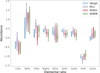 |
Fig. 2 Violin plot. |
6 Results
6.1 Mean abundances
Our analysis yields a mean metallicity of [Fe/H]=–1.04±0.06, which agrees very well with ASCAP DR17, with Ortolani et al. (2019), Vásquez et al. (2018) and Kunder & Butler (2020), as shown in Table 2. On the other hand, Valenti et al. (2010) and Dias et al. (2016) reported a much higher value value, [Fe/H]= –0.65 and –0.79, respectively. Valenti et al. (2010) based their results on the slope of the RGB, while Dias et al. (2016) based their results on low-resolution FORS spectra. In both cases, the difference might be due to the very different technique they used.
We found a dispersion for [Fe/H] of σ=0.06 dex. The total [Fe/H] range we found is 0.16 dex, which is mainly produced by the high metallicity (–0.91) of the star 2M18014656-2751239. By, comparing the observed dispersion with the total error on iron from Table 3 (0.06 dex), however, we found that there is no significant intrinsic iron spread, which makes Djorg 2 consistent with other GCs at similar metallicity, as shown in Figure 2. The observed spread of Ca is0.10 dex (see Table 2), which matches the typical uncertainty (0.08)and indicates no intrinsic spread. Our mean [Mg/Fe] agrees relatively well with ASCAP DR17, Dias et al. (2016) and Kunder & Butler (2020), and our mean [Ca/Fe] agrees with ASCAP DR17.
When we consider Mg, Si, Ca, and Ni as the best α elements, the mean α enhancement of Djorg 2 is
![Mathematical equation: $[\alpha /Fe] = + 0.27 \pm 0.14.$](/articles/aa/full_html/2026/03/aa55637-25/aa55637-25-eq5.png) (1)
(1)
In Fig. 2, we compare the chemical abundances we obtained for Djorg 2 with those of M12, NGC1851 and NGC2808 taken from Mészáros et al. (2019), which have similar metallicity to our cluster. Djorg 2 clearly compares well with the other clusters for Mg and Ca.
For the lightest elements, our mean [C/Fe] and [O/Fe] agree relatively well with those of ASCAP DR17, while Kunder & Butler (2020) gave a mean carbon content that is significantly higher. We found a mean value for [N/Fe] that is significantly lower than either ASCAP DR17 or Kunder & Butler (2020). Compared with M12, NGC1851, and NGC2808, our cluster shows a similar C and O content, but its N abundance is lower on average.
Finally, our [Al/Fe] agrees with ASCAP DR17, but is higher than Kunder & Butler (2020), and it matches the range defined by M12, NGC1851 and NGC2808. The [Ce/Fe] abundances reportes by González-Díaz et al. (2023) is lower than ours, but our cerium content is lower than that of the three comparison clusters (see Figure 2).
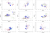 |
Fig. 3 Diagrams pf [N/Fe] vs. [C/Fe], [C/Fe] vs. [O/Fe], [N/Fe] vs. [O/Fe], [Al/Fe] vs. [Mg/Fe], [Al/Fe] vs. [Si/Fe], [N/Fe] vs. [Al/Fe], [Mg/Fe] vs. [Si/Fe], [Ce/Fe] vs. [N/Fe], and [Ce/Fe] vs. [Al/Fe] for Djorg 2 stars (blue stars). The blue, violet, and red circles are stars from other clusters with similar metallicitites to compare our results. The filled symbols represent the star in common with our study. The figure also shows the error bar for each star. |
6.2 Anticorrelations of light and s elements and intrinsic spread
For the other elements affected by MPs, we also considered their possible (anti)correlations. For this purpose, we plot relations between C, N, O, Mg, Al, Si, and Ce in Figure 3. N and C present the typical anticorrelation found in other clusters, and O correlates well with C and anticorrelates with N, but in the last case (O vs. N), the errors prevent us from seeing a more clearer trend. The observed spread is 0.18 dex for C, 0.40 for N, and 0.18 for O, which is well above the typical uncertainties of Table 3. We conclude that C, N, and O present a real abundance variation and that their behavior is consistent with that expected from MPs.
Manganese appears to have no real spread (confirmed by the typical uncertainty of Table 3), while the abudance of Alvaries from [Al/Fe]=+0.17 to [Al/Fe]=+0.57, which is higher than expected from the errors (0.13 dex; see Table 3). Al is also correlated with N. Si and Mg do not correlate with Al or with each other. We do not see the Ce:N or Ce:Al correlations reported by Fernández-Trincado et al. (2022).
To reinforce the statistical significance of the reported correlations, we applied a simple permutation test using the scipy.stats.permutationtest function in Python. This test compares the observed correlation coefficients with the null hypothesis ofno correlation between the abundances. The results are listed below,
N–C: statistic = 0.894, p-value = 0.008
O–C: statistic = 0.608, p-value = 0.004
Al–N: statistic = −0.190, p-value = 0.359
These results confirm that the N–C and O–C anticorrelations are statistically significant, with p-values below 0.01, while the Al–N trend is not significant (p ~ 0.36). This supports the robustness of the multiple-population signatures we report in Djorg 2, despite the limited sample size.
We tested the behavior of [O/Fe] as a function of stellar temperature in order to explore the sensitivity of the OH lines to Teff to Teff. With the original parameters, the oxygen abundances do not display any significant trend with Teff. When we artificially increased the stellar temperatures by +100 K, however, a clear correlation between [O/Fe] and Teff emerged. This confirms that our adopted atmospheric parameters are consistent and reliable, because only the modified set of parameters produces an induced trend. When we lowered the temperature by −100 K, a possible propagation, was observed, but it was not as noticeable as in the first case.
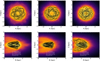 |
Fig. 4 Ensemble of one million orbits in the frame corotating with the bar for Djorg 2, projected on the equatorial (top) and meridional (bottom) Galactic planes in the noninertial reference frame with a bar pattern speed of 31 (left), 41 (middle) and 51 (right) km s−1 kpc−1, and integrated backward in time over 2 Gyr. Yellow and orange show the most probable regions of phase space, which are most frequently crossed by the simulated orbits. The solid black line shows the orbital path of Djorg 2 from the observables without error bars. |
7 Orbit
We made use of the advanced Milky Way model GravPot161 to predict the orbital path of the GC Djorg 2 in a steady-state gravitational Galactic model that includes a boxy/peanut bar structure (Fernández-Trincado et al. 2019). The orbits were integrated with GravPot16, which includes the perturbations due to a realistic (as far as possible) rotating “boxy/peanut” bar, which fits the structural and dynamical parameters of the Galaxy to the currently best known values.
For the orbit computations, we adopted the same model configuration, solar position and velocity vector as described by Fernández-Trincado et al. (2019), except for the angular velocity of the bar (Ωbar), for which we employed the recommended value of 41 km s−1 kpc−1 (Sanders et al. 2019), and we assumed variations of ±10 km s−1 kpc−1. The considered structural parameters of our bar model (e.g., mass and orientation) are within observational estimates that lie in the range of 1.1 × 10¹⁰ M⊙ and present-day orientation of 20° (value adopted from dynamical constraints, as highlighted in Fig. 12 of Tang et al. 2018) in the noninertial frame (where the bar is at rest). The bar scale lengths are x0 =1.46 kpc, y0 = 0.49 kpc, and z0 =0.39 kpc, and the middle region ends at the effective semimajor axis of the bar Rc = 3.28 kpc (Robin et al. 2012).
For guidance, the Galactic convention we adopted was the X-axis oriented toward l = 0° and b = 0°, the Y -axis is oriented toward l = 90° and b =0°, and the disc rotating toward l = 90°; the velocity was also oriented in these directions. Following this convention, the solar orbital velocity vectors are [U⊙, V⊙, W⊙] = [11.1, 12.24, 7.25] km s−1 (Schönrich et al. 2010). The model was rescaled to the galactocentric distance of the Sun, 8.27 kpc (GRAVITY Collaboration 2021), and the circular velocity at the solar position was ~229 km s−1 (Eilers et al. 2019).
The most likely orbital parameters and their uncertainties were estimated using a simple Monte Carlo scheme. An ensemble of one million orbits was computed backward in time for 2 Gyr, under variations of the observational parameters assuming a normal distribution for the uncertainties of the input parameters (e.g., positions, heliocentric distances, radial velocities, and proper motions), which were propagated as 1σ variations in a Gaussian Monte Carlo resampling. To compute the orbits, we adopted a mean radial velocity (RV) of −149.75 ± 1.1 km s−1. The absolute proper motions < μα > and < μδ > were taken from 0.72 and –3.003, with an assumed uncertainty of 0.5 mas yr−1 for the orbit computations. The heliocentric distance (d⊙) was adopted as 11.3 kpc. The results for the main orbital elements are listed in the inset of Figure 4.
Figure 4 shows the simulated orbital path of Djorg 2 by adopting a simple Monte Carlo approach. The probability densities of the resulting orbits are projected on the equatorial and meridional galactic planes, in the noninertial reference frame where the bar is at rest. The black line in the figure shows the orbital path (adopting observables without uncertainties). The yellow color corresponds to the most probable regions of the space, which are crossed more frequently by the simulated orbits. Djorg 2 is clearly confined in a bulge-like orbit, which lies in an in-plane orbit with high eccentricity >0.75 and low vertical (Zmax < 1.6 kpc) excursions from the Galactic plane, and apogalactocentric distances shorter than 1.8 kpc. This cluster extends inside and outside of the bar in the Galactic plane, but not with a bar-shaped orbit, which means that this cluster is not trapped by the bar, and is instead confined to a retrograde orbit. The bulge nature of the orbit of Djorg 2 confirms its classification as a bulge GC by Geisler et al. (in prep.) based on both dynamical and chemical constraints.
The average orbital parameters listed in Figure 4 show that the Galactic bar induces the cluster to have smaller average (peri-/apo-)galactic distances, lower vertical excursions from the Galactic plane, and higher eccentricities, even for any of the bar pattern speed values. This suggests that the effect of different Ωbar on Djorg 2 is almost negligible.
8 Summary and conclusions
We presented a high-resolution (R ~ 22 500) detailed spectral abundance analysis for six stars belonging to the highly reddened GC Djorg 2, which is located in the direction of the inner Galaxy and was obtained as a part of the CAPOS survey. Nine chemical species were examined, including light elements (C and N), α-elements (O, Mg, Si, and Ca), iron-peak elements (Fe, Ti), odd-Z elements (Al), and s-process elements (Ce), using the code BACCHUS. The chemical abundances observed in Djorg 2 are consistent with those of other Galactic GCs (GCs) of similar metallicity (e.g. Mészáros et al. 2019). The main conclusions of this study are summarized below:
The mean metallicity of Djorg 2 is 〈[Fe/H]〉 = −1.04 ± 0.03, with a star-to-star metallicity spread (0.06 dex) that is comparable with the measurement uncertainties;
Clear N–C, O–C and Al–N (anti)correlation trends are observed in Djorg 2. C, N, O. and Al are spread intrinsically, which indicates multiple stellar populations;
No clear intrinsic spread for Mg, Si, or Ce was found;
The orbital analysis showed that Djorg 2 moves inside the Galactic bulge, which makes it a true Bulge GC.
Acknowledgements
S.V. gratefully acknowledges the support provided by Fonde- cyt Regular no. 1220264, and by the ANID BASAL project FB210003. D.G. gratefully acknowledges the support provided by Fondecyt regular no. 1220264. D.G. also acknowledges financial support from the Dirección de Investigación y Desarrollo de la Universidad deLa Serena through the Programa de Incentivo ala Investigación de Académicos (PIA-DIDULS). J.G.F.-T. gratefully acknowledges the grants support provided by ANID Fondecyt Iniciación No. 11220340, ANID Fondecyt Postdoc No. 3230001, and from the Joint Committee ESO-Government of Chile under the agreement 2023 ORP 062/2023.
References
- Ahumada, R., Prieto, C. A., Almeida, A., et al. 2020, AJSS, 249, 3 [Google Scholar]
- Alvarez, R., & Plez, B. 1998, A&A, 330, 1109 [NASA ADS] [Google Scholar]
- Barbuy, B., Chiappini, C., Cantelli, E., et al. 2014, A&A, 570, A76 [NASA ADS] [CrossRef] [EDP Sciences] [Google Scholar]
- Barbuy, B., Chiappini, C., & Gerhard, O. 2018, ARA&A, 56, 223 [Google Scholar]
- Bica, E., Ortolani, S., & Barbuy, B. 2016, PASA, 33, e028 [Google Scholar]
- Bica, E., Ortolani, S., Barbuy, B., & Oliveira, R. A. P. 2024, A&A, 688, A154 [NASA ADS] [CrossRef] [EDP Sciences] [Google Scholar]
- Blanton, M. R., Bershady, M. A., Abolfathi, B., et al. 2017, AJ, 154, 28 [Google Scholar]
- Bressan, A., Marigo, P., Girardi, L., et al. 2012, MNRAS, 427, 127 [NASA ADS] [CrossRef] [Google Scholar]
- Cardelli, J. A., Clayton, G. C., & Mathis, J. S. 1989, ApJ, 345, 245 [Google Scholar]
- Cohen, R. E., Mauro, F., Alonso-García, J., et al. 2018, AJ, 156, 41 [Google Scholar]
- Dias, B., Barbuy, B., Saviane, I., et al. 2016, A&A, 590, A9 [NASA ADS] [CrossRef] [EDP Sciences] [Google Scholar]
- Eilers, A.-C., Hogg, D. W., Rix, H.-W., & Ness, M. K. 2019, ApJ, 871, 120 [Google Scholar]
- Fernández-Trincado, J. G., Beers, T. C., Tang, B., et al. 2019, MNRAS, 488, 2864 [NASA ADS] [Google Scholar]
- Fernández-Trincado, J. G., Villanova, S., Geisler, D., et al. 2022, A&A, 658, A116 [NASA ADS] [CrossRef] [EDP Sciences] [Google Scholar]
- Geisler, D., Villanova, S., O’Connell, J. E., et al. 2021, A&A, 652, A157 [NASA ADS] [CrossRef] [EDP Sciences] [Google Scholar]
- Geisler, D., Parisi, M. C., Dias, B., et al. 2023, A&A, 669, A115 [NASA ADS] [CrossRef] [EDP Sciences] [Google Scholar]
- González-Díaz, D., Fernández-Trincado, J. G., Villanova, S., et al. 2023, MNRAS, 526, 6274 [CrossRef] [Google Scholar]
- GRAVITY Collaboration (Abuter, R., et al.) 2021, A&A, 647, A59 [NASA ADS] [CrossRef] [EDP Sciences] [Google Scholar]
- Gunn, J. E., Siegmund, W. A., Mannery, E. J., et al. 2006, AJ, 131, 2332 [NASA ADS] [CrossRef] [Google Scholar]
- Gustafsson, B., Edvardsson, B., Eriksson, K., et al. 2008, A&A, 486, 951 [NASA ADS] [CrossRef] [EDP Sciences] [Google Scholar]
- Harris, W. E. 2010, arXiv e-prints [arXiv:1012.3224] [Google Scholar]
- Kerber, L. O., Libralato, M., Souza, S. O., et al. 2019, MNRAS, 484, 5530 [Google Scholar]
- Koch, A., McWilliam, A., Preston, G. W., & Thompson, I. B. 2016, A&A, 587, A124 [NASA ADS] [CrossRef] [EDP Sciences] [Google Scholar]
- Kunder, A. M., & Butler, E. 2020, AJ, 160, 241 [NASA ADS] [CrossRef] [Google Scholar]
- Majewski, S. R., Schiavon, R. P., Frinchaboy, P. M., et al. 2017, AJ, 154, 94 [NASA ADS] [CrossRef] [Google Scholar]
- Massari, D., Koppelman, H. H., & Helmi, A. 2019, A&A, 630, L4 [NASA ADS] [CrossRef] [EDP Sciences] [Google Scholar]
- Masseron, T., Merle, T., & Hawkins, K. 2016, BACCHUS: Brussels Automatic Code for Characterizing High accUracy Spectra, Astrophysics Source Code Library [record ascl:1605.004] [Google Scholar]
- Minniti, D., Geisler, D., Alonso-García, J., et al. 2017, AJ, 849, L24 [CrossRef] [Google Scholar]
- Mott, A., Allende Prieto, C., Beers, T. C., et al. 2020, A&A, 636, A85 [NASA ADS] [CrossRef] [EDP Sciences] [Google Scholar]
- Muratov, A. L., & Gnedin, O. Y. 2010, AJ, 718, 1266 [NASA ADS] [Google Scholar]
- Mészáros, S., Masseron, T., García-Hernández, D. A., et al. 2019, MNRAS, 492, 1641 [Google Scholar]
- Nataf, D. M., Gonzalez, O. A., Casagrande, L., et al. 2016, MNRAS, 456, 2692 [Google Scholar]
- Nidever, D. L., Holtzman, J. A., Allende Prieto, C., et al. 2015, AJ, 150, 173 [NASA ADS] [CrossRef] [Google Scholar]
- O’Donnell, J. E. 1994, ApJ, 422, 158 [Google Scholar]
- Ortolani, S., Bica, E., & Barbuy, B. 1997, MNRAS, 284, 692 [NASA ADS] [Google Scholar]
- Ortolani, S., Held, E. V., Nardiello, D., et al. 2019, A&A, 627, A145 [NASA ADS] [CrossRef] [EDP Sciences] [Google Scholar]
- Pérez-Villegas, A., Barbuy, B., Kerber, L., et al. 2019, MNRAS, 491, 3251 [Google Scholar]
- Plez, B. 2012, Turbospectrum: Code for spectral synthesis, Astrophysics Source Code Library [record ascl:1205.004] [Google Scholar]
- Renaud, F., Agertz, O., & Gieles, M. 2016, MNRAS, 465, 3622 [Google Scholar]
- Robin, A. C., Marshall, D. J., Schultheis, M., & Reylé, C. 2012, A&A, 538, A106 [NASA ADS] [CrossRef] [EDP Sciences] [Google Scholar]
- Romero-Colmenares, M., Fernández-Trincado, J. G., Geisler, D., et al. 2021, A&A, 652, A158 [NASA ADS] [CrossRef] [EDP Sciences] [Google Scholar]
- Salaris, M., Chieffi, A., & Straniero, O. 1993, ApJ, 414, 580 [NASA ADS] [CrossRef] [Google Scholar]
- Sanders, J. L., Smith, L., & Evans, N. W. 2019, MNRAS, 488, 4552 [NASA ADS] [CrossRef] [Google Scholar]
- Saracino, S., Dalessandro, E., Ferraro, F. R., et al. 2019, AJ, 874, 86 [Google Scholar]
- Savino, A., Koch, A., Prudil, Z., Kunder, A., & Smolec, R. 2020, A&A, 641, A96 [NASA ADS] [CrossRef] [EDP Sciences] [Google Scholar]
- Schönrich, R., Binney, J., & Dehnen, W. 2010, MNRAS, 403, 1829 [NASA ADS] [CrossRef] [Google Scholar]
- Smith, V. V., & Lambert, D. L. 2013, AJ, 765, 155 [Google Scholar]
- Tang, B., Fernández-Trincado, J. G., Geisler, D., et al. 2018, ApJ, 855, 38 [Google Scholar]
- Valenti, E., Ferraro, F. R., & Origlia, L. 2010, MNRAS, 402, 1729 [NASA ADS] [CrossRef] [Google Scholar]
- VandenBerg, D. A., Brogaard, K., Leaman, R., & Casagrande, L. 2013, AJ, 775, 134 [Google Scholar]
- Vasiliev, E., & Baumgardt, H. 2021, MNRAS, 505, 5978 [NASA ADS] [CrossRef] [Google Scholar]
- Vásquez, S., Saviane, I., Held, E. V., et al. 2018, A&A, 619, A13 [Google Scholar]
All Tables
All Figures
|
Fig. 1 Global properties of the Djorg 2 targets. In all the panels, our targets are represented using a star-symbol. Top left panel: spatial position. The color-coded symbols represent the S/R of the stars (labeled in bottom left panel) with APOGEE spectra. Other APOGEE targets in the field are shown as gray dots. A circle with the tidal radius (Harris 2010) is overplotted. Bottom-left panel: radial velocity vs. metallicity of our members compared to field stars. The black box encloses the cluster members within 0.2 dex and 15 km/s from the nominal mean [Fe/H]=–1.04 dex and RV=–149.8 km/s, as determined in this work. Top-right panel: color–magnitude diagram corrected for differential reddening in the Gaia Bp and 2MASS K bands within 5’. Our targets all lie along the red giant branch. The best isochrone fit is represented by green circles. Field stars are plotted as gray dots. Bottom-right panel: proper motion density distribution of stars located within the tidal radius from the cluster center. The inner plot in the top left corner shows a zoom-in of the cluster squared in 0.7 × 0.7 mas yr−1 and enclosed in a proper motion radius of 0.5 mas yr−1, shown as a blue circle. The dashed gray lines are centered on the cluster center PM values and PM-based cluster members are indicated as yellow circles. |
| In the text | |
|
Fig. 2 Violin plot. |
| In the text | |
|
Fig. 3 Diagrams pf [N/Fe] vs. [C/Fe], [C/Fe] vs. [O/Fe], [N/Fe] vs. [O/Fe], [Al/Fe] vs. [Mg/Fe], [Al/Fe] vs. [Si/Fe], [N/Fe] vs. [Al/Fe], [Mg/Fe] vs. [Si/Fe], [Ce/Fe] vs. [N/Fe], and [Ce/Fe] vs. [Al/Fe] for Djorg 2 stars (blue stars). The blue, violet, and red circles are stars from other clusters with similar metallicitites to compare our results. The filled symbols represent the star in common with our study. The figure also shows the error bar for each star. |
| In the text | |
|
Fig. 4 Ensemble of one million orbits in the frame corotating with the bar for Djorg 2, projected on the equatorial (top) and meridional (bottom) Galactic planes in the noninertial reference frame with a bar pattern speed of 31 (left), 41 (middle) and 51 (right) km s−1 kpc−1, and integrated backward in time over 2 Gyr. Yellow and orange show the most probable regions of phase space, which are most frequently crossed by the simulated orbits. The solid black line shows the orbital path of Djorg 2 from the observables without error bars. |
| In the text | |
Current usage metrics show cumulative count of Article Views (full-text article views including HTML views, PDF and ePub downloads, according to the available data) and Abstracts Views on Vision4Press platform.
Data correspond to usage on the plateform after 2015. The current usage metrics is available 48-96 hours after online publication and is updated daily on week days.
Initial download of the metrics may take a while.