| Issue |
A&A
Volume 707, March 2026
|
|
|---|---|---|
| Article Number | A131 | |
| Number of page(s) | 15 | |
| Section | Planets, planetary systems, and small bodies | |
| DOI | https://doi.org/10.1051/0004-6361/202556031 | |
| Published online | 16 March 2026 | |
Asteroid characterization using Gaia Data Release 3
I. Shapes, spins, and scattering properties
1
Department of Physics, University of Helsinki,
PO Box 64,
00014
Finland
2
Astronomical Observatory Institute, Faculty of Physics, A. Mickiewicz University,
Sloneczna 36,
60-286
Poznan,
Poland
3
INAF – Osservatorio Astrofisico di Torino,
10025
Pino Torinese,
Italy
4
Université Côte d’Azur, Observatoire de la Côte d’Azur,
CNRS, Laboratoire Lagrange,
France
5
Yunnan Observatories, Chinese Academy of Sciences,
Kunming,
China
★ Corresponding author: This email address is being protected from spambots. You need JavaScript enabled to view it.
Received:
19
June
2025
Accepted:
11
December
2025
Abstract
Context. The third Gaia data release (DR3) contains high-precision, sparse-in-time brightness measurements of over 150000 asteroids.
Aims. We employed a light-scattering inversion technique to estimate the rotation periods, spin pole orientations, shapes, and photometric phase function parameters (slope and absolute magnitude) of over 8000 asteroids based solely on DR3 photometry.
Methods. Using triaxial ellipsoid and convex shapes, we sought the best-fit shape, spin, and linear slope, along with their uncertainties, via a Markov chain Monte Carlo sampling technique. We also fit H,G12 and H,G1,G2 phase functions from predicted brightnesses derived from the fit shapes. Using previously reported diameters, the Gaia G-band geometric albedos were calculated. Variations in the spin and shape properties were assessed among various families and background populations of the Main Belt.
Results. We found that for the vast majority of our objects the best-fit ellipsoid spin poles are comparable to that of a convex shape. We rejected 15% of convex shapes and used the acceptable solutions to investigate differences in the shape distribution of families in the Main Belt. Revisiting the amplitude phase relationship, we found a strong dependence on the shape b/a elongation. The Bond albedo was calculated from the phase integral and shown to correlate well with the G12 slope parameter and known taxonomic classifications. The G-band absolute magnitudes and geometric albedos are systematically fainter than V-band values.
Conclusions. The assumption of ellipsoid shape for sparse datasets is sufficient for estimating the spin pole longitude and latitude. We find no correlation between the shapes and spins of main-belt asteroid families and their ages. Absolute magnitudes and phase functions derived from Gaia photometry should be favored over the V band when estimating the solar energy budget, such as in thermal modeling applications. Asteroid taxonomies can be assessed to some degree from the photometric slopes and albedos.
Key words: methods: numerical / methods: statistical / catalogs / minor planets, asteroids: general
© The Authors 2026
 Open Access article, published by EDP Sciences, under the terms of the Creative Commons Attribution License (https://creativecommons.org/licenses/by/4.0), which permits unrestricted use, distribution, and reproduction in any medium, provided the original work is properly cited.
This article is published in open access under the Subscribe to Open model. This email address is being protected from spambots. You need JavaScript enabled to view it. to support open access publication.
1 Introduction
Measurements of an asteroid's brightness as a function of time (i.e., its lightcurve, LC) can be used to estimate the shape and spin properties. The utility of photometric inversion techniques (e.g., Kaasalainen & Torppa 2001; Kaasalainen et al. 2001) to constrain the spin and shape properties of asteroids from densein- time ground-based LCs has been extensively demonstrated over the past few decades (Ďurech et al. 2015). Inversion methods have traditionally been applied to dense-in-time ground-based LCs, but the inclusion of sparse-in-time photometry has also shown to be effective at constraining the model parameters (Kaasalainen 2004). Shape and spin solutions from combination of these dense and sparse datasets for thousands of asteroids has been compiled in the database for asteroid models through inversion techniques (DAMIT; Ďurech et al. 2010). The aim of this extensive study is to assess the shape and spin properties of asteroids in order to derive insights about their past evolution. The change in brightness as a function of the solar phase angle (or simply, the phase angle) is described by the phase function and is a result of the scattering properties of the surface. The phase function for asteroids has evolved from the two parameter H,G function (Bowell et al. 1989) into the three-parameter function H,G1,G2 (Muinonen et al. 2010) that comprises the absolute magnitude, H, and the phase-curve parameters G1 and G2. Accurate estimation of these parameters requires precise photometry collected over a sufficiently large range of phase angles. The nonspherical shapes of asteroids complicate the estimation of phase function parameters when LC effects are not properly accounted for. Therefore, phase function parameter estimates are more precise when photometric inversion properly accounts for shape and viewing geometry effects (Muinonen et al. 2020). For sparsely sampled photometric datasets, the H,G12 or H,G*12 can be used (Muinonen et al. 2010; Penttilä et al. 2016) and a linear function with a constant slope on the magnitude scale is applicable for cases when the phase-angle coverage is between approximately 10 to 50° - the region where changes in the magnitude are essentially directly proportional to the phase angle. Successful fitting of these models to Gaia DR2 data suggests that asteroid taxonomy can be broadly assessed from phase function parameters (Martikainen et al. 2021).
The high-precision sparse-in-time photometry measured by the Gaia space telescope has enabled studies of asteroid shapes, spins (Ďurech & Hanuš 2018, 2023; Cellino et al. 2024), and photometric phase functions (Martikainen et al. 2021 ; Muinonen et al. 2022) across a few data releases. The most recent data release 3 catalog (DR3) contains photometric observations of more than 150 000 asteroids collected during a 34-month period (Tanga et al. 2023). Here we use DR3 brightness measurements to estimate shape and spin parameters along with their uncertainties for a large corpus of asteroids. Using the approach outlined in Muinonen et al. (2020), we fit simple triaxial ellipsoids and general convex shapes to estimate the rotational periods, spin axes, and photometric slopes of the asteroids in our sample. In this approach, both systematic and random uncertainties are accounted for via a Markov chain Monte Carlo (MCMC) sampler that utilizes randomly generated virtual observations, and updates the parameter probability distributions from best-fit solutions.
The rest of the article is organized as follows. In Sect. 2 we introduce the Gaia DR3 asteroid data together with the methods used, in Sect. 3 we analyze the results in a broad context, and in Sect. 4 we conclude our findings.
2 Materials and methods
2.1 Gaia DR3
We downloaded the full DR3 dataset and processed the photometric observations by first averaging over transits. The Gaia brightness measurements are processed as magnitudes, rather than fluxes, in our model. The precision is often better than 0.01 mag. The photometric measurements represent the integrated brightness within the so-called Gaia G-band filter, which differs from most passband often used in other photometric surveys. We will return to this point in our analysis of the results.
From the full set of DR3 photometry, we first selected asteroids that have 30 or more Gaia photometric observations. This selection criterion gives over 22 000 asteroids, with nearly all of them being main-belt asteroids. For any given asteroid, its Gaia observations span a phase angle range (Δα) within typically 10° to 30° and were acquired serendipitously within the 36 month long survey. We follow up on the independent study of Cellino et al. (2024) in which shape and spin properties were determined using a genetic algorithm applied to DR3 data. As a result, the number of objects considered herein will dramatically reduce, as we apply some quality filters described in the next subsection and in Section 3.
2.2 Photometric modeling
Results from the genetic evolution algorithm presented by Cellino et al. (2024) were used to give the initial rotation period, spin pole, and ellipsoid shape values for a set of 8670 asteroids. This truncated list was a result of applying rejection filters based on various criteria that rule out physically unrealistic solutions (Cellino et al. 2024). These include filtering out unreasonably low and high photometric slopes, rotation periods of less than 2.1 h, extreme shape and spin pole values, and large model residuals.
We first employed triaxial ellipsoid shapes as described by the semimajor axes for which a ≥ b ≥ c. A Lommel-Seeliger surface scattering model is employed, as was done in Cellino et al. (2024), for which the integrated brightness can be computed analytically. Using the ellipsoid shape and spin solutions as initial conditions, convex shapes described by the Gaussian surface density were then fit to the observations. In both shape assumptions, a photometric phase function was used that assumes linear dependence on the phase angle (Muinonen et al. 2022). Thus, a linear phase slope, β0, was used in the shape fitting procedure in lieu of H,G1,G2 phase function (Muinonen et al. 2010) and we performed post hoc phase function fits in the observed reference geometry using the optimized shape as described below. We sampled the probability distribution of each model parameter by using an MCMC approach (Muinonen et al. 2020) to generate a set of 5000 solutions. We describe these aspects of our modeling approach in more detail throughout this subsection.
2.2.1 Surface scattering model
To model the surface brightness, we made use of the Lommel-Seeliger surface reflection coefficient (Muinonen et al. 2022)
 (1)
(1)
where ι and ε refer to the angles of incidence and emergence as measured from the outward normal vector of a surface element, φ denotes the azimuth angle, and α is the phase angle. Additionally, p is the geometric albedo and Φ11 is the single-scattering phase function,
 (2)
(2)
For phase angles 10° ≤ α ≤ 50°, a linear model can be utilized for modeling the disk-integrated phase function, Φ:
 (3)
(3)
where it is explicitly stated that the photometric slope at α = 20° then equals the parameter β0.
2.2.2 Inverse problem
As for the ellipsoid shape model, the parameters (model unknowns) of the forward model are described by the vector
 (4)
(4)
where the NP = 7 free parameters are the rotation period, ecliptic pole longitude, ecliptic pole latitude, rotational phase at an arbitrary reference epoch t0, two ellipsoid axial ratios (with a > b > c denoting the semiaxes), and the single parameter of the phase function. Furthermore, we do not permit the b/a and c/a axial ratios to exceed below 0.4 in the ellipsoid inversion.
In the case of the convex shape model, the parameters are
 (5)
(5)
where the shape is described by the  spherical harmonics coefficients s00,..., slmaxlmax for the Gaussian surface density. Here φ0 and the real-valued s00 can be fixed as the rotational phase is immersed in the spherical harmonics coefficients and the asteroid size information is omitted. Thus, the total number of parameters equals
 (6)
(6)
We chose a maximum degree of lmax = 4 and lmin = 0 to represent the convex shapes, meaning that we have 24 parameters to describe the shape model alone and 28 total parameters for each asteroid.
The Bayesian formulation of the inverse problem in magnitude space together with observational error model is described by Muinonen et al. (2022). An MCMC method for characterizing the multidimensional probability density of the free parameters is given by Muinonen et al. (2020), with a thorough description of the so-called virtual least squares solutions for setting up the MCMC proposal probability density. The reader is referred to these two publications for more details about the inverse methods used herein.
2.2.3 Phase function, absolute magnitude, and albedo modeling
Following the computation of the best-fit convex shape solutions, we estimated the best-fit H,G12 phase function of the predicted LC maxima at the observation dates and the H,G1,G2 phase function that corresponds to a spherical asteroid with the surface reflection coefficient equivalent to that derived for the convex shape. For further details about these two phase functions, the reader is referred to Muinonen et al. (2010). This is achieved only by changing the phase function, Φ(α), in Equation (2). Consequently, three parameters are solved for: the absolute magnitude, H, and two phase-curve shape parameters, G1, G2. We note here that our phase function fitting is in accordance with the magnitude-space fitting by Penttilä et al. (2016), which differs from previous implementations of the phase curve fitting in flux space (i.e., Muinonen et al. 2010; Oszkiewicz et al. 2011).
In order to map the G1, G2 regime of physical relevance, we made use of the parameters
 (7)
(7)
The maximum value of  is dictated by the fact that G1 + G2 ≤ 1, whereas the minimum value of
  roughly corresponds to an opposition effect amplitude of 0.5 mag,
  . Likewise, the minimum and maximum values of G|| correspond roughly to half of the relevant values of the G12-parameter (Muinonen et al. 2022).
The absolute magnitude, HGaia, was computed from the H,G12 phase function fit using the predicted mean brightnesses of the best-fit convex shape solution. Note, however, that the H,G1,G2 and H,G12 photometric phase functions have been developed for phase curves corresponding to maximum LC brightness and, consequently, the photometric slopes of equivalent spherical objects are typically larger (i.e., steeper phase curves) than those of nonspherical convex shapes. These absolute magnitudes thus imitate those for a spherical asteroid with projected area equivalent to the mean projected area of the convex shape. As a consequence, the absolute magnitudes using the convex shapes and H,G12 are brighter (i.e., smaller values).
Additionally, we calculated G-band geometric albedos, pGaia, from the absolute magnitudes and using the diameters Deff that are reported in the Solar System Open Database Network (SsODNet; Berthier et al. 2023) and using the relationship (Russell 1916; Pravec & Harris 2007) derived in Appendix A:
![Mathematical equation: \sqrt{p_{\Gaia}} = \dfrac{1246\ \textrm{km}\ 10^{-0.2H_{\Gaia}}}{D_{\mathit{eff}} [\textrm{km}]} ,](/articles/aa/full_html/2026/03/aa56031-25/aa56031-25-eq12.png) (8)
(8)
where it is noted that the scaling factor in the numerator is based on the Gaia magnitude of the Sun in the Vega System (Casagrande & VandenBerg 2018). We consider the SsODNet values to be robust aggregation across multiple reported diameters from infrared surveys and occultations observations across many publications. The object sizes, given by Deff, is that of a sphere having the same projected area as a Lambertian disk when viewed face-on (Appendix A). We emphasize that these pGaia values are derived parameters not calculated from the LC inversion procedure.
3 Results and analysis
We eliminated objects for which the quality of fit was not improved by the convex shape assumption from the ellipsoid fit. We also filtered out objects with rms > 0.1 mag for the convex shape assumption. From this rms filtering, we eliminated 393 objects (4.5% of the starting set) and are left with 8277 asteroids. Our object set includes 7947 main-belt asteroids, 46 Hungaria region asteroids, 283 Hildas and Jupiter Trojans, and 3 nearEarth objects. Full results can be accessed at the CDS and a list of the various fit parameters and associated uncertainties derived from both the ellipsoid inversion (EI) and convex shape inversion (CXI) for (16) Psyche is given in Appendix B. Figure B.1 shows the number of Gaia observations used across this set of objects, as well as the range in phase angles for each object. The spin period, pole latitude, and pole longitude uncertainties obtained from ellipsoids and convex shapes are compared in Figure B.2. In the case of the rotation period, the relative uncertainty is calculated: σProt/Prot. In most cases, the uncertainties are smaller when using convex shapes when compared to ellipsoids. The most straightforward explanation is that the greater number of free parameters used for convex shapes (24 shape parameters) allows for better fits to the observations.
3.1 Spins and shapes
The rotation periods of the ellipsoids and convex shape models are almost exactly identical for all objects, with some extreme outliers (Figure 1). This agreement is most likely due to the fact that the initial set of parameters used for both shape inversion methods are taken from the already computed best-fit ellipsoid parameters from Cellino et al. (2024). If we had run an independent search for rotation periods for each shape assumption, then each would likely find different solutions in many cases. Having nearly identical periods for both shapes is an opportunity to more systematically study the effects of shape assumption on other model parameters, as is discussed below. Our rotation periods are compared to previous works that used photometry from the Transiting Exoplanet Survey Satellite (TESS) in Figure C.1. We discuss in Appendix C that our results agree to within 1% for 67.3% and 45.6% of the solutions in Pál et al. (2020) and McNeill et al. (2023), respectively. The inconsistent agreement is likely due to the different methodologies used in these works.
We compare the ecliptic coordinates of the pole longitudes and latitudes in Figures 1b and c. Most solutions are in agreement, most fall within 15° around the one-to-one matches shown by the red line. Spin latitudes show a dearth of spin poles near 0°, with fewer ellipsoid solutions than convex solutions. The spin longitudes show in Figure 1b have a more broadly uniform agreement for both shape assumptions. We see that, for 4% of the objects, the difference between the ellipsoid and convex spins are greater than 90°, representing values closer to the 180° mirrored solutions. The agreement of the ellipsoid and convex shape spin poles may suggest some level of stability in the search for the minimization of model fit residuals. However, because of the sparse nature of the Gaia observations, it is likely that these spin periods and poles do not always represent the global best-fit (Cellino et al. 2024).
The comparison of convex shapes to ellipsoid shapes is nontrivial. Whereas ellipsoids are specified by two ratios of their semiaxes, convex shapes are parameterized by multiple spherical harmonic coefficients (Sect. 2.2.2). To overcome this challenge, a 3D shape was generated from the set of spherical harmonics calculated in the best-fit nominal solution for each object (Kaasalainen et al. 1992b,a). We then found the set of ellipsoid parameters that yield a minimum  value by utilizing the downhill simplex method. We compared the b/a and c/a axis ratios of the fit ellipsoid, referred to as b/acxi and c/acxi to that of the ellipsoid shapes directly fit to the DR3 photometry in Figs. 1d and e. Many objects closely follow the one-to-one correspondence, shown by red lines, but large discrepancies are apparent.
In order to compare the ellipsoid and convex model parameter fits, we calculated the Akaike information criterion statistic (AIC) as
 (9)
(9)
where NGaia is the number of observations. The AIC takes into account the different number of model parameters ( and
and  ) and the root-mean-square values (rmsei and rmscxi for ellipsoids and convex shapes, respectively) of the fit. The convex model is penalized more for having more free parameters so the AIC is useful for comparing the quality of fits between two models that have differences in the number of free parameters. For our purpose, the difference is computed as ΔAIC = AICcxi - AICei and shown in Figure 1f. The ΔAIC distribution shows a wide range of values that span in the approximate range from −50 to +150. Positive values designate larger AICcxi values, indicating that the convex shape approximation offers a more robust fit over the ellipsoid shape for that object.
The peak of the ΔAIC distribution occurs essentially at zero, suggesting that these objects are equally fit using the ellipsoid and convex shapes. Approximately 38% of the ΔAIC distribution has negative values which signify that the DR3 data for these objects are overfit using a convex shape assumption. Using the ΔAIC values we searched for potential relationships with the number of Gaia observations and with the phase angle sampling for each object. Neither of these observational parameters could explain differences in the AIC. One explanation could simply be that some fraction of asteroids are shaped more closely to ellipsoids. On the other hand, the low number of sparse data, compared to dense LCs, may not be suitable to conclude this. Follow-up work could investigate how the number of shape parameters (i.e., Equation (6)) can be optimized for the quality and quantity of photometric data (e.g., Figure 3 from Ďurech & Hanuš 2023).
The distribution of  values as a function of b/acxi and c/acxi ratios is shown in Figure 2. We find a grouping of shapes with more extreme axial ratios that we deem suspect and chose to remove them from our analysis. The acceptable shapes are shown as green points in both panels, and the criteria as dashed red lines in the top panel: c/acxi > 0.2,
  , and
, and  . As a consequence of these conditions, many objects with lower values of b/acxi are also removed. The true shapes of the objects that do not meet this criteria could be highly nonconvex, such as a contact binary shape, or represent a binary system, both of which exhibit large shifts in LC amplitude as the viewing aspect angle changes. We searched for, but found no relationship to the ΔAIC, suggesting that the rejected objects are indifferent to both shape assumptions. It has been shown that a convex shape model can compensate for real-world nonconvexity with large, flat areas (e.g., Kaasalainen et al. 2002) which would cause the entire shape to depart significantly from an ellipsoid and increase the effective elongation.
Our shape filter criteria rejects 1267 of the 8277 objects that had passed our root mean square (rms)-based criteria, signifying that the convex (and ellipsoid) shape assumption is not applicable for around 15% of our successful model runs. This fraction is, coincidentally, within a factor or two of the estimated near-Earth contact binary population (Virkki et al. 2022). Future investigations could use similar methods of flagging highly non-convex shapes or binary systems for follow-up investigation using dense LC observations (Ďurech & Kaasalainen 2003). Finally, we note that while these convex shapes were removed from further use, we utilized their spin properties (i.e., rotation period and spin axis longitude and latitude) and photometric slopes for our analysis.
A commonly cited issue in shape inversion is that shapes are not well constrained along the direction of the rotation axis (i.e., the c axis for an ellipsoid) unless observations sample a sufficient range of viewing aspects (Kaasalainen et al. 1992b). Similarly, information about the elongations (i.e., the b/a axis ratio) require sufficient sampling of the LC in order to establish constraints on its amplitude. Notably, the constraints on the b/a ratio are comparable to that of the c/a ratio, which is likely due to the fact that we are using only sparse in time observations. If a dense LC with tens of data points were to be considered, then the elongation will be known to a much higher precision.
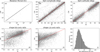 |
Fig. 1 Comparison between (a) rotation periods, (b) spin axis longitudes, (c) spin axis latitudes, (d) b/a axis ratio, (e) c/a axis ratios, and (f) the ΔAIC statistic (Equation (9)) for ellipsoid (EI) and convex (CXI) shape assumptions. |
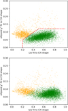 |
Fig. 2 The |

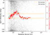 |
Fig. 3 Spin obliquity and rotation period for 8277 objects. The rolling mean (using a window of N = 200 objects) of the prograde abundance as a function of rotation period is given. |
3.1.1 Population trends
For each asteroid, we transformed the spin pole orientation into coordinates defined by its orbital plane. In this coordinate system, the spin obliquity is akin to the latitude in ecliptic coordinates and is defined as zero for a prograde rotator with a spin pole that is perpendicular to the orbital plane. We also defined a spin longitude relative to a reference direction that we choose to be the orbital perihelion. In doing this transformation, we can investigate the variations in spin orientation across our sample.
The distribution of spin poles among the main-belt asteroid population is of great interest (Ďurech & Hanuš 2023). We calculated the overall ratio of prograde to retrograde rotators in our entire sample to be 52% which, given the large sample size (N = 8248), is statistically significant (p value < .001). We also find that the spin obliquity distribution is nonuniform with respect to rotation period. This relationship is shown in Figure 3 in which the mean prograde to retrograde ratio with rotation period is also given. The peak abundance of prograde rotators of ~60% occurs at a rotation period of approximately 20 hours. An excess of prograde rotators has been observed for asteroids with sizes larger than 150 km (Kryszczyńcska et al. 2007), which may be a leftover feature from the accretion of protoplanets in the early Solar System (Takaoka et al. 2023). The bulk of our object set samples the size range from 3 to 20 km, so it is not clear if this spin fingerprint can be retained for collisionally evolved objects.
A barely detectable excess of retrograde rotators can be seen for rotation periods near 4 h in Figure 3. As the majority of diameters in our set are <20 km, the YORP-driven evolution is a likely explanation (Vokrouhlický & Čapek 2002) and agrees with previous modeling work (e.g., Hanuš et al. 2011). At slower rotation rates the abundance of retrograde rotators reaches a maximum at around 55% that is statistically significant at the 95% confidence (3σ) level. Slowly rotating asteroids with periods longer than 100 hours may likely be in a tumbling state (Zhou et al. 2025), but the sparse in time Gaia photometry precludes detection of non-principal axis (NPA) rotation. At slower rotation rates, a statistically significant excess of retrograde rotators is seen at around 55% at the 95% confidence (3σ) level. Slowly rotating asteroids with periods longer than 100 h may likely be in a tumbling (i.e., NPA) rotation state as a result of collisional evolution (Zhou et al. 2025). However, sparse-in-time photometry precludes the detection of NPA rotation and independent followup work is needed to confirm the spin poles of slow rotators (e.g., Marciniak et al. 2021).
We show the distribution of shapes as a function of rotation period Figure 4. For objects with rotation periods shorter than approximately 5 hours, there is a strong tendency toward rounder shapes; that is, higher b/acxi. This trend is likely a consequence of reshaping via local structural failure (i.e., Hirabayashi et al. 2020). As the spin rate of an asteroid over longer timescales is driven by the YORP effect, differences in the internal friction and the internal structural properties can lead to different shape outcomes (Walsh et al. 2012). On average our convex shapes near the spin barrier approach axial ratios of b/acxi ~ 0.8 and c/acxi ~ 0.60, which corresponds roughly to an intermediate internal fraction angle of 20° used by Walsh et al. (2012) to model the reshaping due to YORP spinup. Thus, these rounder objects may represent a surviving population, as rotational disruption events could cause elongated objects to become rounder or disrupted at high spin rates (Hirabayashi & Scheeres 2019).
We searched for, but did not find, a significant size-dependent variation in the convex shapes that has been seen in other works. For example, Cibulková et al. (2016) found that asteroids in the Lowell Database larger than 50 km were more rounded, but no changes in the shape distribution were apparent below this size. This non-result may be due to the size range represented among the objects, as 95% of our objects are in the size range of 2 to 100 km. The average distribution of b/a ellipsoid axial ratios was previously approximated using Gaia DR2 observations, assuming prolate spheroids (c/a = b/a), by Mommert et al. (2018). Instead of explicitly fitting ellipsoid shapes, the authors found an average b/a = 0.80 ± 0.04 using a statistical approach (i.e., McNeill et al. 2016). Our analysis shows a lower average value of b/acxi ≈ 0.7 (Figure 4) that suggests more elongated shapes, on average. In the work of Ďurech & Hanuš (2023), inversion methods were used on the DR3 dataset. A different subset of objects was analyzed compared to this work, and the authors found that, on average, smaller asteroids (<20 km) and faster rotators (< 4 hours) are increasingly elongated.
The spin and shape distributions of asteroid families has been the subject of recent studies (Nortunen et al. 2017; Cibulková et al. 2018; Szabó et al. 2022; Ďurech & Hanuš 2023). Thus, we analyze here the asteroids in our sample based on family membership. We focus on the family lists published by Nesvornÿ et al. (2015) found in the Planetary Data System Small Bodies Node. We also select members of the Eulalia and new Polana families identified by Walsh et al. (2013) and treat the remaining asteroids of the Nysa-Polana complex as members of the Nysa family that consists of high-pv asteroids. The members of a primordial inner-belt (PIB) family are acquired by first removing all members contained within the Nesvornÿ et al. (2015) family lists, then cross-referencing the remaining objects that have been marked as “certain” (code 1 or 2) in the supplementary file from Delbo et al. (2017).
We divided the background asteroid population into respective regions in the Main Belt based on their orbital semimajor axis: inner (2.05 au < a < 2.5 au), middle (2.5 au < a < 2.82 au), and outer (2.82 au < a < 3.27 au). Although the Hun-garia family is considered dynamically separate from the Main Belt (Bottke et al. 2012), we include it along with the inner families. Several prior works show that trends exist between family ages and spin frequency and/or shape elongation. We analyzed the spin and shape cumulative distributions for families having 30 or more objects in our sample, of which there are 22 in total, in Figure 5. Partly following Ďurech & Hanuš (2023), we filtered out rotation periods longer than 48 hours (0.5 cycles/day), leaving some families with fewer than 30 spin rate values, as is indicated in each panel. In order to remove clutter and provide a more appropriate comparison, we broke down families into their respective main-belt regions (inner, middle, and outer). There are six families each in the inner Main Belt (IMB) and middle Main Belt (MMB), and ten families in the outer Main Belt (OMB).
We find statistically significant differences in the distributions of spin rates and shapes between all of the background populations. The significance is signified by p values of <.05 in all cases. This suggests that the differences in shape and spin properties of asteroids is partly influenced by the heliocentric distance, or the distinct collisional environments within each region, or both. In addition, the brightness-limited nature of the Gaia survey itself introduces a size-dependent bias in the observed properties of asteroid families across different regions. Furthermore, the broad compositional gradient of the Main Belt (DeMeo & Carry 2014) adds complexity to identifying the key factors that affect shape and spin. Direct comparisons of asteroid family properties and interpretations of these differences should therefore be made with caution.
From a visual inspection of the CDFs in Figure 5, we observe a larger dispersion of spin rates between families in the MMB and OMB regions. We employed the Kolmogorov-Smirnov (K-S) test to assess differences between the spin distributions of each family and their respective background population, and find the following statistically different cases (with p value <.05): IMB-Flora (.047), MMB-Gefion (.014), MMB-Adeona (.030), OMB-Koronis (.034), OMB-Veritas (.007), OMB-Eos (.045), OMB-Ursula (.023), and OMB-Euphrosene (.018). We repeated the K-S tests across the same groups using their shape distributions and identify the following differences: IMB-Vesta (.037), MMB-Dora (.028), MMB-Adeona (.020), and OMB-Hygeia (.007). Out of this list, the Adeona family stands out as being unique in both the spin rate and shape elongation distributions. Contrary to previous works, we do not find a direct relationship between the spin and shape properties with family age (e.g., the very young Veritas and ancient Ursula families have similar spin and shape distributions). We therefore suggest a more complex interplay between multiple factors, such as the age, composition, and the collisional environment determined by the location in the Main Belt (e.g., Szabó & Kiss 2008), which influence the observed shape and spin distributions. However, a rigorous treatment that accounts for multiple contributing factors goes beyond the scope of this work. Future efforts should investigate the inclusion of additional effects simultaneously, for example.
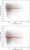 |
Fig. 4 Convex shape axial ratios b/acxi (top) and c/acxi (bottom) as a function of rotation period for 7010 objects. Boxcar moving averages using a window of N = 200 objects are shown as red lines. |
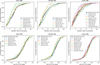 |
Fig. 5 Cumulative distributions of the rotation frequency (top) and b/a fits to convex shapes (bottom) for families and background populations in the inner (left panels), middle (middle panels), and outer (right panels) Main Belt. |
3.1.2 Parallels to regolith grain size trends
We note that trends between spins and shapes just mentioned have been identified for surface regolith grain sizes by MacLennan & Emery (2022), in which smaller particles were found for asteroid diameters smaller than 10 km. The authors suggest this relationship is a consequence of the change in strength of asteroids at 10 km that affects the ejecta particle sizes. In our study, we could not find any size dependence with the shape properties but we identified a change for fast rotators (Figure 4). MacLennan & Emery (2022) also found that fast rotators with Prot < 5 hours have larger regolith particles, which may be caused by particle ejections as a result of spin-up evolution via the YORP effect. Regolith cohesion experiments indicate that failure is more likely for coarse grains because of increased internal friction via grain interlocking (Brisset et al. 2022), which is consistent with the scarcity of finer regolith for fast rotators. Elongated fast rotators are more susceptible to structural failure at locations further from the spin axis where centrifugal forces are highest (e.g., Guibout & Scheeres 2003). These aforementioned analyses of asteroid shapes and regolith properties is encouraging for establishing links between asteroid interior properties with their external characteristics (e.g., Zhang et al. 2022). We encourage future investigations to focus on characterization of the relationship between the shapes, spins, and regolith properties of a greater number of asteroids by combining optical and infrared datasets (e.g., Ďurech et al. 2015; Marciniak et al. 2021).
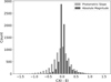 |
Fig. 6 Distributions of the differences between the best-fit ellipsoid and convex shape photometric slopes (mag/rad) and absolute magnitudes (mag). |
3.2 Scattering properties
3.2.1 Photometric phase slope
The photometric slopes determined from ellipsoid and convex shape fits to each shape are compared in Figure 6. The distribution of photometric phase slope uncertainties are shown in panel f of Figure B.2. The distribution of slope differences (CXI minus EI) has a standard deviation of around 0.31 mag rad−1, but shows broad agreement, on average, between the two shape assumptions with a mean of −0.02 mag rad−1. Similarly, the distribution of absolute magnitude differences agree with a mean and standard deviation of 0.02 ± 0.17 mag. Generally speaking, photometric phase curve parameters are more accurate when using fit shape and spin parameters, as opposed to a spherical assumption, because rotational variations and aspect changes (Jackson et al. 2022) at different observing geometries are accounted for. Our results demonstrate that, for sparse Gaia photometry, the differences between the phase function parameter fits are minimal for our two shape assumptions. Our results are also relevant for the application of the recent photometric phase curve model called “sH,G1 ,G2” (Carry et al. 2024), which account for brightness changes due to changing aspect angle of an oblate shape.
Throughout this work, we utilized the photometric slopes that are based on the mean LC brightness (i.e., means-based). We also calculated and used here the photometric slope based on the maximum LC brightness (max-based) and calculated the difference between these two photometric slopes. The difference can be used only as a proxy for the changes in amplitude with phase angle, as we did not explicitly calculate the amplitude. Hereafter, we refer to this parameter as the pseudo-amplitude-phase relationship (pAPR), given in units of mag/rad. Larger values of the APR imply a steeper increase in the LC amplitude and negative values imply a decrease in amplitude at larger phase angles. Recent work suggests that the pAPR is chiefly dependent on the spin obliquity (Gutiérrez et al. 2006); however, we show that the shape elongation (given by b/acxi) is the dominant factor in Figure 7. A clear inverse linear relationship is shown in our dataset in which elongated shapes (smaller b/acxi) exhibit larger pAPR values. Additionally, we observe a small increase in the pAPR for more extreme spin obliquities (i.e., those that deviate from 90°). Finally, we also observe a detectable, but minor decrease in the pAPR for larger G12 values, implying a weak dependence on the surface scattering properties such as the albedo. Our results suggest that, for the phase angles covered by the DR3 dataset (10° < α < 30°), the amplitude-phase relationship is chiefly dictated by the shape properties and, to a lesser extent, the spin obliquity, as proposed in previous works (Zappala et al. 1990; Gutiérrez et al. 2006).
The albedo and slope parameter have been shown to be useful in estimating an asteroid’s taxonomic type when there is a lack of spectral or color information. For example, MacLennan & Emery (2022) combined the phase curve parameter from the two-parameter H,G phase function with derived geometric albedos in order to assess the likely taxonomic groups of asteroids without spectral data. We depict Bond albedos and G12 values derived herein in the left panel of Figure 8. For applicable objects we show the taxonomy from the Mahlke classification system (Mahlke et al. 2022), which incorporates spectral and albedo information in a probabilistic classification framework. The classes show more distinct separation in the albedo dimension, as compared to G12. In the Mahlke system, the low-albedo (C, Ch, P, and D) classes are well separated from high-albedo (S, V, and E) classes. Moderate albedo (L, K, and M) classes form an overlapping continuum, making them harder to distinguish. We also show four T-type asteroids from the Bus-DeMeo taxonomy that have consistently moderate albedos.
We show the G|| versus G⊥ values calculated from Equation 7 in Figure 9. These two parameters were derived from H,G1 ,G2 phase curve fits to the max-based LC brightness that was calculated from the best-fit convex shape model for each object. The green, piecewise linear function represents the equivalent G12 parameters, which are also fit using the maximum LC brightness. Our Gaia sample is shown as gray points on this plot and closely follow the green function. The effect of using the mean LC brightness is shown as shifts indicated by the arrows (both by the magnitude and direction) at each G12 marker. In the H,G1,G2 and H,G12 systems, Martikainen et al. (2021) showed that the use of mean LC brightness values can shift the fit G1, G2, and G12 values, blurring the tenuous boundaries between taxonomic groups. Considering that the uncertainties are typically smaller, we suggest that albedo is a better indicator of taxonomic type over the photometric slope.
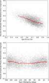 |
Fig. 7 Relationship between our pseudo-amplitude-phase relationship as a function of the b/a elongation of convex shapes (top: b/acxi), the same relationship as a function of the spin obliquity (bottom). A running mean of N = 200 is shown in red. |
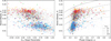 |
Fig. 8 Bond albedos (AGaia) and G12 slope parameters (left) and Gaia Bond albedos as a function of the phase integral q (right), with lines showing Gaia geometric albedos (pGaia). Both panels show objects for which the taxonomy is available from SsODNet. |
3.2.2 Absolute magnitude
The absolute magnitudes from the convex shapes are slightly skewed toward somewhat larger values (Figure 6). When comparing the convex G-band absolute magnitudes to V-band absolute magnitudes in the Lowell Photometric Database (Oszkiewicz et al. 2011; Bowell et al. 2014), the Gaia based absolute magnitudes are 0.37 mag larger on average (Figure 10). To assess this difference, we consider the difference between the filters, as the Gaia G-band magnitude of the Sun is around 0.15 mag fainter than in the V band. However, this can only partly explain the discrepancy between absolute magnitudes. Another possible explanation is the methods by which the phase functions were calculated (flux versus magnitude based) or the limited phase angle coverage (e.g., see Figure B.1).
We also computed absolute magnitudes of the H,G*12 system (Penttilä et al. 2016), which are also derived from the G1 and G2 parameters. This system differs fundamentally from the H,G12 in that the bright E-types were not considered due to their G1 and G2 values that differ from the overall trend seen among other taxonomic types (Muinonen et al. 2010). Consequently, objects with β0 < 1.5 have increasingly different treatment of the opposition effect that determines the absolute magnitude. This difference can be seen in the bottom panel of Figure 9, as smaller G⊥ (and G1) implies a stronger opposition effect, subsequently lowering the absolute magnitudes in the H,G*12 system for objects with low photometric slopes. To mitigate confusion in reporting absolute magnitude, we instead provide the difference in the magnitude of the opposition effect between the two systems,  , to be added to HGaia in order to calculate the appropriate H,G*12 absolute magnitude.
3.2.3 Albedo and phase integral
The phase integral, q, is defined as the ratio of the Bond albedo to the geometric albedo. In the H,G1,G2 system, (Muinonen et al. 2010) q is computed from
 (10)
(10)
We used these phase integrals and our absolute magnitude estimates to derive the geometric and Bond albedos of asteroids in our dataset. Only 6504 objects are included in this analysis because diameters are not available for the entire set. For the distribution of q for various known taxonomic groups see Figure 8.
The bolometric Bond albedo, A, for asteroids in the Solar System is calculated as the amount of solar radiation that is reflected across all wavelengths and phase angles. It is an important quantity that is used in thermal modeling to compute the incoming solar radiation (insolation) for an asteroid surface. In practice, the Bond albedo is often approximated using the radiometrically derived size and absolute magnitude via the geometric albedo (Delbo et al. 2015), which is most commonly provided for the Johnson V filter (Hoffmann et al. 2025). However, only a small portion of the incident solar spectrum is accounted for in this bandpass (e.g., Myhrvold 2018). The wide Gaia passband covers visible, ultraviolet, and near-infrared wavelengths, spanning a wavelength range of 300-1000 nm and completely encompasses the Johnson UBVR and SDSS ugriz sets of filters. We therefore recommend that, whenever possible, G-band absolute magnitudes and phase slopes be used for purposes of albedo calculation from the object size (Eqs. (8) and (10)).
Comparing our G-band albedos against those aggregated by SsODNet (Berthier et al. 2023), we find strong agreement overall, but a high skew toward lower Gaia albedos (Figure 10). This result is not likely due to the may be related to differences in the absolute magnitudes for the different filters (e.g., Masiero et al. 2021). Independent follow-up work should seek to explicitly confirm this interpretation.
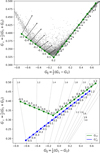 |
Fig. 9 G⊥ versus G|| green line shows the G12 relationship with marked values. Top : objects in our dataset calculated from G1 and G2 derived from H,G12 fits. Arrows extending from the G12 relationship indicate the approximate corresponding shift when LC maxima are used. Bottom : the gray lines show the photometric slopes (β0) from 1.0 to 3.0 mag/rad in 0.2 increments. The theoretical G12 relationship is shown as the blue line. |
3.2.4 Main Belt families and background populations
We take from the family membership criteria mentioned above in Section 3.1.1. Unfortunately, there are not enough objects from several families, including the PIB family, but accounting of family members is essential for this analysis. Analyzing the distributions of photometric slopes within and across each family, we first tested the albedo modality of families included in Table 1 and find that they are all unimodal. The albedo distributions of the IMB and OMB background populations were found to be bimodal, consisting of low primitive and moderate siliceous albedos. The means of each slope distribution and mean geometric albedos for families are also given in Table 1. A strong inverse correlation is apparent between slope and the log10 of the albedo for the families and for the background populations alike. Background populations show a positive trend between heliocentric distance and slope (and an inverse relationship with albedo).
Next, we tested whether the distribution of Gaia geometric albedos are statistically distinguishable from the regional background population using the K-S test of their albedo cumulative distribution functions. The results of these tests are listed as p-value statistics in Table 1. The results indicate that all but two families considered have distinct albedo distributions: Nysa and Baptistina. Many studies have used albedos and colors to identify likely background interlopers and separate overlapping families (e.g., Ivezić et al. 2002; Parker et al. 2008; Masiero et al. 2013; Dykhuis & Greenberg 2015). Such approaches rely on accurate and precise albedos and assume families that are homogeneous in albedo and that are different from the local background population. We therefore encourage future works to consider the photometric slopes for identifying or eliminating candidate members of asteroid families.
The population of background asteroids in the Main Belt likely represent scattered fragments of primordial planetesimals that were destroyed in the early Solar System. Additionally, dynamical instability has caused most of the original mass of the Main Belt to be lost (Morbidelli et al. 2015). The orbits of the remaining fragments of these primordial families have dispersed such that there is essentially no reliable way to identify clusters of orbital elements (Brasil et al. 2016; Carruba et al. 2016). It has been shown that Hungaria family members exhibit distinct albedo distributions and spectral types from the background objects that represent remnants of a so-called E-belt (Lucas et al. 2019). Future prospects could involve searching for small clusters of asteroids with statistically different albedo and photometric slopes as compared to other objects in the same region. On the other hand it is not clear how, or if, photometric slopes can or should be reliably utilized in this way. Furthermore, the uncertainties in slope from this Gaia dataset are larger than for albedo, making them less practical for comparisons among individual objects.
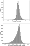 |
Fig. 10 Comparison of absolute magnitudes with those from the Lowell Database (top; Oszkiewicz et al. 2011) and comparison of geometric albedos with those reported in SsODNet (bottom; Berthier et al. 2023). |
Comparison of main-belt family slope and albedo distributions against the respective regional background population.
4 Conclusions
We used the Gaia DR3 photometry to successfully determine the photometric phase slopes, shapes, and spin properties of 8467 asteroids using triaxial ellipsoids and general convex shapes. The assumption of ellipsoid shape for sparse datasets is sufficient for estimating the spin pole longitude and latitude. Additionally, ellipsoid models are sufficient for determination of phase function parameters (absolute magnitude and slope) with convex shapes offering little advantage for sparse data. The inclusion of at least one dense LC in a photometric inversion model would justify the use of a convex shape.
There exists a significant fraction of slow rotators in our sample, consistent with other works using Gaia photometry. These slow rotators have similar shape properties to the remaining population, but faster rotators (5 < hours) have rounder shapes. There exists a slight but statistically significant excess of prograde rotators (52%) in the general asteroid population and YORP-driven evolution has resulted in more retrograde rotators at the fastest and slowest spin rates. Our methods assumes a principal axis rotation, so any slowly rotating tumblers are not properly modeled. Future shape inversion efforts with Gaia photometry should utilize additional datasets such as LCs in order to assess a tumbling state.
We do not find evidence that the shape and spin distributions of main-belt asteroid families are correlated with their ages. However, some asteroid families exhibit statistically distinguishable spin frequency and shape elongations compared to the background population. These differences are likely due to an interplay between different ages, collisional environments, and compositions.
The amplitude phase relationship - the increase in amplitude with the solar phase angle - was reassessed using the photometric slopes based on calculated LC maxima and means. We found that the relationship is dictated by the b/a axis ratio in which the amplitude of more elongated shapes exhibits a stronger dependence on the phase angle. Simplistic phase function models that do not perform full photometric inversion can incorporate this finding to assess the shape and spin properties. Following our analysis of the H,G1, G2 phase function parameters, we suggest a reformulation to bring about a unified assessment of S and E-types, respectively.
The extremely wide bandpass of the G-band filter is a unique aspect of the Gaia mission compared to other surveys. We find our derived absolute magnitudes (HGaia) to be systematically fainter than those in the V band calculated from the Lowell Photometric Database. In congruence with this result, the Gaia geometric albedos (pGaia) calculated herein are smaller than those compiled by the SsODNet service. We claim that the phase integral (q) derived from G-band photometry is more physically appropriate for calculation of the Bond albedo (A) required for estimation of the solar energy budget for use in thermal models. Lastly, we show that major taxonomic complexes can be distinguished, to a certain degree, using the photometric slopes and albedos. Our companion paper explores taxonomic classification using Gaia DR3 spectra in combination with our albedo and photometric slopes in more detail.
Data availability
The full results are available at the CDS via https://cdsarc.cds.unistra.fr/viz-bin/cat/J/A+A/707/A131.
Acknowledgements
This work has made use of data from the European Space Agency (ESA) mission Gaia (https://www.cosmos.esa.int/gaia), processed by the Gaia Data Processing and Analysis Consortium (DPAC). Funding for the DPAC has been provided by national institutions, in particular the institutions participating in the Gaia Multilateral Agreement. The authors wish to thank the Finnish Computing Competence Infrastructure (FCCI) for supporting this project with computational and data storage resources. This research has made use of IMCCE’s SsODNet VO service (https://ssp.imcce.fr/webservices/ssodnet/). E.M.M. is supported by the Research Council of Finland grant No. 353784. The research has also been supported by the Research Council of Finland grants No. 336546, No. 347627, and No. 359893. K.M. and A.P. acknowledge support from Foreign Experts Project (FEP), State Administration of Foreign Experts Affairs of China (SAFEA), with contract No. H20240864. D.O. acknowledges financial support from grant No. 2022/45/B/ST9/00267 from the National Science Centre, Poland.
References
- Berthier, J., Carry, B., Mahlke, M., & Normand, J. 2023, A&A, 671, A151 [NASA ADS] [CrossRef] [EDP Sciences] [Google Scholar]
- Bottke, W. F., Vokrouhlický, D., Minton, D., et al. 2012, Nature, 485, 78 [NASA ADS] [CrossRef] [Google Scholar]
- Bowell, E., Hapke, B., Domingue, D., et al. 1989, in Asteroids II, eds. R. P. Binzel, T. Gehrels, & M. S. Matthews, 524 [Google Scholar]
- Bowell, E., Oszkiewicz, D. A., Wasserman, L. H., et al. 2014, Meteor. Planet. Sci., 49, 95 [Google Scholar]
- Brasil, P. I. O., Roig, F., Nesvornÿ, D., et al. 2016, Icarus, 266, 142 [NASA ADS] [CrossRef] [Google Scholar]
- Brisset, J., Sánchez, P., Cox, C., et al. 2022, Planet. Space Sci., 220, 105533 [CrossRef] [Google Scholar]
- Carruba, V., Nesvornÿ, D., Aljbaae, S., Domingos, R. C., & Huaman, M. 2016, MNRAS, 458, 3731 [Google Scholar]
- Carry, B., Peloton, J., Le Montagner, R., Mahlke, M., & Berthier, J. 2024, A&A, 687, A38 [NASA ADS] [CrossRef] [EDP Sciences] [Google Scholar]
- Casagrande, L., & VandenBerg, D. A. 2018, MNRAS, 479, L102 [NASA ADS] [CrossRef] [Google Scholar]
- Cellino, A., Tanga, P., Muinonen, K., & Mignard, F. 2024, A&A, 687, A277 [NASA ADS] [CrossRef] [EDP Sciences] [Google Scholar]
- Cibulková, H., Ďurech, J., Vokrouhlický, D., Kaasalainen, M., & Oszkiewicz, D. A. 2016, A&A, 596, A57 [NASA ADS] [CrossRef] [EDP Sciences] [Google Scholar]
- Cibulková, H., Nortunen, H., Ďurech, J., et al. 2018, A&A, 611, A86 [NASA ADS] [CrossRef] [EDP Sciences] [Google Scholar]
- Delbo, M., Mueller, M., Emery, J. P., Rozitis, B., & Capria, M. T. 2015, in Asteroids IV, eds. P. Michel, F. E. DeMeo, & W. F. Bottke (Arizona University Press), 107 [Google Scholar]
- Delbo, M., Walsh, K., Bolin, B., Avdellidou, C., & Morbidelli, A. 2017, Science, 357, 1026 [NASA ADS] [CrossRef] [Google Scholar]
- DeMeo, F. E., & Carry, B. 2014, Nature, 505, 629 [NASA ADS] [CrossRef] [Google Scholar]
- Ďurech, J., & Hanuš, J. 2018, A&A, 620, A91 [NASA ADS] [CrossRef] [EDP Sciences] [Google Scholar]
- Ďurech, J., & Hanuš, J. 2023, A&A, 675, A24 [NASA ADS] [CrossRef] [EDP Sciences] [Google Scholar]
- Ďurech, J., & Kaasalainen, M. 2003, A&A, 404, 709 [NASA ADS] [CrossRef] [EDP Sciences] [Google Scholar]
- Ďurech, J., Sidorin, V., & Kaasalainen, M. 2010, A&A, 513, A46 [Google Scholar]
- Ďurech, J., Carry, B., Delbo, M., Kaasalainen, M., & Viikinkoski, M. 2015, in Asteroids IV, eds. P. Michel, F. E. DeMeo, & W. F. Bottke (University of Arizona Press), 183 [Google Scholar]
- Dykhuis, M. J., & Greenberg, R. 2015, Icarus, 252, 199 [NASA ADS] [CrossRef] [Google Scholar]
- Guibout, V., & Scheeres, D. J. 2003, Celest. Mech. Dyn. Astron., 87, 263 [Google Scholar]
- Gutiérrez, P. J., Davidsson, B. J. R., Ortiz, J. L., Rodrigo, R., & Vidal-Nuñez, M. J. 2006, A&A, 454, 367 [NASA ADS] [CrossRef] [EDP Sciences] [Google Scholar]
- Hanuš, J., Ďurech, J., Broz, M., et al. 2011, A&A, 530, A134 [NASA ADS] [CrossRef] [EDP Sciences] [Google Scholar]
- Hirabayashi, M., Nakano, R., Tatsumi, E., et al. 2020, Icarus, 352, 113946 [Google Scholar]
- Hirabayashi, M., & Scheeres, D. J. 2019, Icarus, 317, 354 [Google Scholar]
- Hoffmann, T., Micheli, M., Cano, J. L., et al. 2025, Icarus, 426, 116366 [NASA ADS] [CrossRef] [Google Scholar]
- Ivezić, Z., Lupton, R. H., Jurić, M., et al. 2002, AJ, 124, 2943 [CrossRef] [Google Scholar]
- Jackson, S. L., Rozitis, B., Dover, L. R., et al. 2022, MNRAS, 513, 3076 [NASA ADS] [CrossRef] [Google Scholar]
- Kaasalainen, M. 2004, A&A, 422, L39 [NASA ADS] [CrossRef] [EDP Sciences] [Google Scholar]
- Kaasalainen, M., & Torppa, J. 2001, Icarus, 153, 24 [NASA ADS] [CrossRef] [Google Scholar]
- Kaasalainen, M., Lamberg, L., & Lumme, K. 1992a, A&A, 259, 333 [NASA ADS] [Google Scholar]
- Kaasalainen, M., Lamberg, L., Lumme, K., & Bowell, E. 1992b, A&A, 259, 318 [Google Scholar]
- Kaasalainen, M., Torppa, J., & Muinonen, K. 2001, Icarus, 153, 37 [NASA ADS] [CrossRef] [Google Scholar]
- Kaasalainen, M., Torppa, J., & Piironen, J. 2002, A&A, 383, L19 [NASA ADS] [CrossRef] [EDP Sciences] [Google Scholar]
- Kryszczyńcska, A., La Spina, A., Paolicchi, P., et al. 2007, Icarus, 192, 223 [NASA ADS] [CrossRef] [Google Scholar]
- Lucas, M. P., Emery, J. P., MacLennan, E. M., et al. 2019, Icarus, 322, 227 [NASA ADS] [CrossRef] [Google Scholar]
- MacLennan, E. M., & Emery, J. P. 2022, PSJ, 3, 47 [Google Scholar]
- Mahlke, M., Carry, B., & Mattei, P. A. 2022, A&A, 665, A26 [NASA ADS] [CrossRef] [EDP Sciences] [Google Scholar]
- Marciniak, A., Ďurech, J., Ali-Lagoa, V., et al. 2021, A&A, 654, A87 [NASA ADS] [CrossRef] [EDP Sciences] [Google Scholar]
- Martikainen, J., Muinonen, K., Penttilä, A., Cellino, A., & Wang, X. B. 2021, A&A, 649, A98 [NASA ADS] [CrossRef] [EDP Sciences] [Google Scholar]
- Masiero, J. R., Mainzer, A. K., Bauer, J. M., et al. 2013, ApJ, 770, 7 [Google Scholar]
- Masiero, J. R., Wright, E. L., & Mainzer, A. K. 2021, PSJ, 2, 32 [NASA ADS] [Google Scholar]
- McNeill, A., Fitzsimmons, A., Jedicke, R., et al. 2016, MNRAS, 459, 2964 [Google Scholar]
- McNeill, A., Gowanlock, M., Mommert, M., et al. 2023, AJ, 166, 152 [NASA ADS] [CrossRef] [Google Scholar]
- Mommert, M., McNeill, A., Trilling, D. E., Moskovitz, N., & Delbo, M. 2018, AJ, 156, 139 [NASA ADS] [CrossRef] [Google Scholar]
- Morbidelli, A., Walsh, K. J., O’Brien, D. P., Minton, D. A., & Bottke, W. F. 2015, in Asteroids IV, eds. P. Michel, F. E. DeMeo, & W. F. Bottke (Arizona University Press), 493 [Google Scholar]
- Muinonen, K., Belskaya, I. N., Cellino, A., et al. 2010, Icarus, 209, 542 [Google Scholar]
- Muinonen, K., Torppa, J., Wang, X. B., Cellino, A., & Penttilä, A. 2020, A&A, 642, A138 [EDP Sciences] [Google Scholar]
- Muinonen, K., Uvarova, E., Martikainen, J., et al. 2022, Front. Astron. Space Sci., 9, 821125 [NASA ADS] [CrossRef] [Google Scholar]
- Myhrvold, N. 2018, Icarus, 303, 91 [Google Scholar]
- Nesvornÿ, D., Broz, M., & Carruba, V. 2015, in Asteroids IV (University of Arizona Press), 297 [Google Scholar]
- Nortunen, H., Kaasalainen, M., Ďurech, J., et al. 2017, A&A, 601, A139 [NASA ADS] [CrossRef] [EDP Sciences] [Google Scholar]
- Oszkiewicz, D. A., Muinonen, K., Bowell, E., et al. 2011, J. Quant. Spec. Radiat. Transf., 112, 1919 [NASA ADS] [CrossRef] [Google Scholar]
- Pál, A., Szakáts, R., Kiss, C., et al. 2020, ApJS, 247, 26 [CrossRef] [Google Scholar]
- Parker, A., Ivezić, Ž., Jurić, M., et al. 2008, Icarus, 198, 138 [Google Scholar]
- Penttilä, A., Shevchenko, V. G., Wilkman, O., & Muinonen, K. 2016, Planet. Space Sci., 123, 117 [Google Scholar]
- Pravec, P., & Harris, A. W. 2007, Icarus, 190, 250 [CrossRef] [Google Scholar]
- Russell, H. N. 1916, ApJ, 43, 173 [Google Scholar]
- Szabó, G. M., & Kiss, L. L. 2008, Icarus, 196, 135 [CrossRef] [Google Scholar]
- Szabó, G. M., Pál, A., Szigeti, L., et al. 2022, A&A, 661, A48 [NASA ADS] [CrossRef] [EDP Sciences] [Google Scholar]
- Takaoka, K., Kuwahara, A., Ida, S., & Kurokawa, H. 2023, A&A, 674, A193 [NASA ADS] [CrossRef] [EDP Sciences] [Google Scholar]
- Tanga, P., Pauwels, T., Mignard, F., et al. 2023, A&A, 674, A12 [NASA ADS] [CrossRef] [EDP Sciences] [Google Scholar]
- Virkki, A. K., Marshall, S. E., Venditti, F. C. F., et al. 2022, PSJ, 3, 222 [Google Scholar]
- Vokrouhlický, D., & Čapek, D. 2002, Icarus, 159, 449 [CrossRef] [Google Scholar]
- Walsh, K. J., Richardson, D. C., & Michel, P. 2012, Icarus, 220, 514 [NASA ADS] [CrossRef] [Google Scholar]
- Walsh, K. J., Delbó, M., Bottke, W. F., Vokrouhlický, D., & Lauretta, D. S. 2013, Icarus, 225, 283 [NASA ADS] [CrossRef] [Google Scholar]
- Zappala, V., Cellino, A., Barucci, A. M., Fulchignoni, M., & Lupishko, D. F. 1990, A&A, 231, 548 [NASA ADS] [Google Scholar]
- Zhang, Y., Michel, P., Barnouin, O. S., et al. 2022, Nat. Commun., 13, 4589 [NASA ADS] [CrossRef] [Google Scholar]
- Zhou, W.-H., Michel, P., Delbo, M., et al. 2025, Nat. Astron., 9, 493 [Google Scholar]
Appendix A Absolute magnitude, diameter, and albedo relationship
Starting from the definition of geometric albedo, p, which is the ratio of observed flux compared to that of an ideal Lambertian disk observed at opposition:
 (A.1)
(A.1)
The conservation of energy implies that the incident flux, Fo, on a reflecting Lambertian disk of area  must equal the reflected flux, Fld(α, Δ), integrated across all phase angles, α ∈ [0,π∕2], on the surface of a hemisphere with a radius Δ:
 (A.2)
(A.2)
From the definition of a Lambertian reflection function,
 (A.3)
(A.3)
thus:
 (A.4)
(A.4)
Integrating the above equation we get:
 (A.5)
(A.5)
and placing this into A.1 yields,
 (A.6)
(A.6)
The incident solar flux is a function of the solar flux at 1 au (F⊙1AU) and the heliocentric distance given in AU (RAU):
 (A.7)
(A.7)
so, in general,
 (A.8)
(A.8)
since the observed flux is phase angle dependent as described by the phase function, Φ(α). Next, using the relationship between magnitude and flux we get
 (A.9)
(A.9)
For α = 0°, Δ = 1 au = 1.495 × 10⁸ km and Rau = 1 then
 (A.10)
We adopted the apparent Gaia-band magnitude of the Sun as m⊙1au = −26.90 (Casagrande & VandenBerg 2018) and, using Deff = 2rld, we arrived at
![Mathematical equation: 1246\ \textrm{km}\ 10^{-H_\textit{Gaia}/5} = p^{1/2}_\textit{Gaia}\ D_\mathit{eff}\ [\textrm{km}].](/articles/aa/full_html/2026/03/aa56031-25/aa56031-25-eq34.png) (A.11)
(A.11)
It is noted that the factor of 1246 km is different from that when using V-band m⊙1au of −26.76, which corresponds to a factor of 1329 km (corresponding to a diameter difference of around 6%).
Appendix B Results tables
Two results tables for ellipsoid and convex shape fits are shown here for (16) Psyche. The full results can be accessed at the CDS.
In Figure B.1 are the distributions of the number of Gaia observations, as well as the range in phase angles for the 8277 objects studied in this work.
Ellipsoid shape parameters of (16) Psyche
Convex shape parameters of (16) Psyche
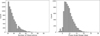 |
Fig. B.1 Distributions of the number of Gaia observations (left) and the per object range of phase angles (right), Δα, for the filtered set of N = 8277 objects. |
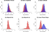 |
Fig. B.2 Parameter uncertainty distributions for triaxial ellipsoids (red) and convex shapes (blue) for (a) the rotation period, (b) spin pole longitudes, (c) spin pole latitudes, (d) photometric phase curve slope, as well as (e) ellipsoid axial ratios b/a and (f) c/a. The rotation periods are expressed as relative uncertainties via σProt/Prot. |
Appendix C Comparison to TESS rotation periods
 |
Fig. C.1 Comparison of the rotation periods estimated from TESS photometry and those reported in this work. Left: Periods for 820 objects from our work that appear in Pál et al. (2020). Right: Periods for 707 objects common to this work and McNeill et al. (2023). |
The Transiting Exoplanet Survey Satellite (TESS) is a mission designed to detect LC signatures of planets transiting other stars. Therefore, like Gaia , TESS conducts untargeted observations of asteroids and both surveys represents a homogeneous sample of the population. However, the TESS photometry are taken over a single epoch and can consist of hundreds of points, as opposed to the sparse data acquired by Gaia . Here, we compare the rotation periods estimated by Pál et al. (2020) and McNeill et al. (2023) with our DR3 results. We use the term “agreement” to indicate solutions within 1%.
There are 820 objects in our work with rotation periods in Pál et al. (2020), of which 552 agree (67.3%). On the other hand, 324 of the 707 (45.8%) objects common to McNeill et al. (2023) have periods in agreement, a striking difference. Between these two works 80% have periods that are “consistent” among the 1119 objects common to both (McNeill et al. 2023).
Of the 526 objects with rotation periods estimated in this work and these two, 276 (52.5%) are in agreement and 87 (16.5%) objects have disparate rotation periods in all three. Our DR3 periods agree with either work in 77.9% of cases (410 objects) and only 29 (9.2%) of period solutions agree between these two works but which are in disagreement with our results. A set of 218 objects have inconsistent periods between the two TESS-based publications, of which 117 (53.7%) from Pál et al. (2020) and 10 (8.5%) from McNeill et al. (2023) are in agreement with our work. This strengthens the claim that our results are more in line with Pál et al. (2020).
All Tables
Comparison of main-belt family slope and albedo distributions against the respective regional background population.
All Figures
|
Fig. 1 Comparison between (a) rotation periods, (b) spin axis longitudes, (c) spin axis latitudes, (d) b/a axis ratio, (e) c/a axis ratios, and (f) the ΔAIC statistic (Equation (9)) for ellipsoid (EI) and convex (CXI) shape assumptions. |
| In the text | |
|
Fig. 2 The |
| In the text | |
|
Fig. 3 Spin obliquity and rotation period for 8277 objects. The rolling mean (using a window of N = 200 objects) of the prograde abundance as a function of rotation period is given. |
| In the text | |
|
Fig. 4 Convex shape axial ratios b/acxi (top) and c/acxi (bottom) as a function of rotation period for 7010 objects. Boxcar moving averages using a window of N = 200 objects are shown as red lines. |
| In the text | |
|
Fig. 5 Cumulative distributions of the rotation frequency (top) and b/a fits to convex shapes (bottom) for families and background populations in the inner (left panels), middle (middle panels), and outer (right panels) Main Belt. |
| In the text | |
|
Fig. 6 Distributions of the differences between the best-fit ellipsoid and convex shape photometric slopes (mag/rad) and absolute magnitudes (mag). |
| In the text | |
|
Fig. 7 Relationship between our pseudo-amplitude-phase relationship as a function of the b/a elongation of convex shapes (top: b/acxi), the same relationship as a function of the spin obliquity (bottom). A running mean of N = 200 is shown in red. |
| In the text | |
|
Fig. 8 Bond albedos (AGaia) and G12 slope parameters (left) and Gaia Bond albedos as a function of the phase integral q (right), with lines showing Gaia geometric albedos (pGaia). Both panels show objects for which the taxonomy is available from SsODNet. |
| In the text | |
|
Fig. 9 G⊥ versus G|| green line shows the G12 relationship with marked values. Top : objects in our dataset calculated from G1 and G2 derived from H,G12 fits. Arrows extending from the G12 relationship indicate the approximate corresponding shift when LC maxima are used. Bottom : the gray lines show the photometric slopes (β0) from 1.0 to 3.0 mag/rad in 0.2 increments. The theoretical G12 relationship is shown as the blue line. |
| In the text | |
|
Fig. 10 Comparison of absolute magnitudes with those from the Lowell Database (top; Oszkiewicz et al. 2011) and comparison of geometric albedos with those reported in SsODNet (bottom; Berthier et al. 2023). |
| In the text | |
|
Fig. B.1 Distributions of the number of Gaia observations (left) and the per object range of phase angles (right), Δα, for the filtered set of N = 8277 objects. |
| In the text | |
|
Fig. B.2 Parameter uncertainty distributions for triaxial ellipsoids (red) and convex shapes (blue) for (a) the rotation period, (b) spin pole longitudes, (c) spin pole latitudes, (d) photometric phase curve slope, as well as (e) ellipsoid axial ratios b/a and (f) c/a. The rotation periods are expressed as relative uncertainties via σProt/Prot. |
| In the text | |
|
Fig. C.1 Comparison of the rotation periods estimated from TESS photometry and those reported in this work. Left: Periods for 820 objects from our work that appear in Pál et al. (2020). Right: Periods for 707 objects common to this work and McNeill et al. (2023). |
| In the text | |
Current usage metrics show cumulative count of Article Views (full-text article views including HTML views, PDF and ePub downloads, according to the available data) and Abstracts Views on Vision4Press platform.
Data correspond to usage on the plateform after 2015. The current usage metrics is available 48-96 hours after online publication and is updated daily on week days.
Initial download of the metrics may take a while.