| Issue |
A&A
Volume 707, March 2026
|
|
|---|---|---|
| Article Number | A273 | |
| Number of page(s) | 13 | |
| Section | The Sun and the Heliosphere | |
| DOI | https://doi.org/10.1051/0004-6361/202557221 | |
| Published online | 17 March 2026 | |
Three-dimensional kink modes in solar coronal slabs: Group velocities and their implications for impulsively excited waves
1
Shandong Key Laboratory of Space Environment and Exploration Technology, Institute of Space Sciences, Shandong University, Weihai 264209, China
2
Center for Integrated Research on Space Science, Astronomy, and Physics, Institute of Frontier and Interdisciplinary Science, Shandong University, Qingdao 266237, China
★ Corresponding author: This email address is being protected from spambots. You need JavaScript enabled to view it.
Received:
12
September
2025
Accepted:
4
February
2026
Abstract
Context. Little attention has been paid to group velocities of three-dimensional (3D) magnetohydrodynamic (MHD) waves in solar coronal seismology.
Aims. This study presents a comprehensive examination of the group velocities of trapped 3D kink modes in coronal slabs, emphasizing the connection of mode analysis to both mode characterization and impulsively excited 3D kink waves.
Methods. We worked in linear, ideal, pressureless MHD, and took the equilibrium slab to be symmetrically structured only in one transverse direction. The dispersion relation was numerically solved, and the results were understood by making in-depth analytical progress. We addressed both the transverse fundamental and its first overtone.
Results. We developed a three-subgroup scheme for categorizing 3D kink modes on the plane spanned by the axial and out-of-plane wavenumbers. The group (vgr) and phase velocities (vph) lie on the same side of the equilibrium magnetic field (B0) for the B0-same-side A and B0-same-side F subgroups, which are further discriminated by the directional similarity of vgr and B0. The B0-straddling subgroup is peculiar in that vgr and vph lie astride B0, a feature that cannot be found for waves in unbounded uniform media in pressureless MHD. This B0-straddling subgroup pertains to both the fundamental and its overtones. We further place our results in the context of impulsive waves, employing the method of stationary phase to predict the large-time wavefront morphology in the plane of symmetry of the equilibrium slab. Wavefronts directed toward B0 derive exclusively from B0-straddling modes, and are confined to narrow sectors.
Conclusions. The directional information of impulsively excited 3D wavefronts carries rich seismic information, whose inversion requires a thorough understanding of the behavior of group velocities of 3D modes.
Key words: magnetohydrodynamics (MHD) / waves / Sun: corona / Sun: magnetic fields
© The Authors 2026
 Open Access article, published by EDP Sciences, under the terms of the Creative Commons Attribution License (https://creativecommons.org/licenses/by/4.0), which permits unrestricted use, distribution, and reproduction in any medium, provided the original work is properly cited.
This article is published in open access under the Subscribe to Open model. This email address is being protected from spambots. You need JavaScript enabled to view it. to support open access publication.
1. Introduction
The past two decades have witnessed a rapid accumulation of observations on low-frequency waves and oscillations in the solar corona (see, e.g., Banerjee et al. 2007; De Moortel & Nakariakov 2012; Shen et al. 2022, for reviews). These observations have largely been placed in two contexts, one being the problem of coronal heating (see the reviews by, e.g., Parnell & De Moortel 2012; Arregui 2015; Van Doorsselaere et al. 2020) and the other being solar coronal seismology (SCS; see, e.g., Nakariakov & Kolotkov 2020; Nakariakov et al. 2024, for reviews). Whichever the application, theoretical investigations into linear magnetohydrodynamic (MHD) waves in structured media often prove indispensable. The transverse structuring is of particular interest given the filamentary nature of the observed wave hosts (see, e.g., Erdélyi & Goossens 2011; Nakariakov et al. 2022; Kolotkov et al. 2023, for topical issues).
We focus on how the transverse structuring influences wave dispersion, by which we specifically mean the distinction between the phase and group velocities. This distinction has long been of theoretical interest in SCS, and tends to be largely addressed for the response of some density-enhanced equilibria to impulsive localized exciters (see, e.g., the reviews by Nakariakov & Kolotkov 2020; Li et al. 2020). We consider one-dimensional (1D) equilibria, for which the density structuring is restricted to only one transverse direction. We let 2D motions refer to those that prohibit wave propagation in the extra transverse direction. It has been customary to examine 2D fast sausage motions to bring out the dispersive effects in slab or cylindrical geometry (e.g., Roberts et al. 1983, 1984; Edwin & Roberts 1988). Impulsively excited sausage motions were predicted to possess a telltale three-phase signature in their time sequences sampled sufficiently far from the exciters (Roberts et al. 1983). An almost monochromatic periodic phase appears first, followed by a stronger quasi-periodic phase and eventually by a monochromatic decay phase (see Edwin & Roberts 1986, for theoretical reasons). This three-phase behavior turns out to be compatible with 2D time-dependent simulations (e.g., Murawski & Roberts 1993, 1994). Likewise, the predicted periodicities were compatible with the observed pulsating behavior in radio bursts (e.g., Zhao et al. 1990; Fu et al. 1990) and visible forbidden line intensities (e.g., Pasachoff & Landman 1984; Pasachoff & Ladd 1987). Seismology was therefore enabled, yielding such key coronal parameters as the transverse Alfvén time (e.g., Roberts et al. 1984; Fu et al. 1990).
Considerable progress has been made for the dispersive evolution of impulsively excited waves in the new century. For instance, Nakariakov et al. (2004) showed that the three-phase signature in time sequences translates into “crazy tadpoles” in the associated Morlet spectra. Some subtleties notwithstanding, the expected temporal or Morlet features were shown to largely persist regardless of the details of the initial exciter (e.g., Goddard et al. 2019; Kolotkov et al. 2021) or the wave host (e.g., Nakariakov et al. 2005; Jelinek & Karlicky 2010; Pascoe et al. 2013; Yu et al. 2016, 2017; Guo et al. 2022; Shi et al. 2025, 2026). That these features tend to be robust is not surprising, given the robust applicability to large-time signals of the method of stationary phase (MSP; Edwin & Roberts 1986; Li et al. 2023). The scenario of impulsive waves has therefore been broadly invoked for or implicated in understanding the oscillatory behavior observed in the radio (e.g., Mészárosová et al. 2009; Kaneda et al. 2018) and visible passbands (e.g., Williams et al. 2001; Katsiyannis et al. 2003; Samanta et al. 2016). Likewise, instances in line with this scenario have been found in imaging data; two examples are the cyclic transverse displacements of streamer stalks (streamer waves; e.g., Chen et al. 2010; Kwon et al. 2013; Decraemer et al. 2020), and the quasi-periodic fast propagating waves (QFPs; Liu et al. 2010, 2011; Shen & Liu 2012).
This study is intended to offer an in-depth mode analysis of 3D kink motions in coronal slabs. Of particular interest are two questions, namely how wave dispersion is influenced by the inclusion of the third dimension, and the spatio-temporal features that can be expected for impulsive 3D kink motions. To our knowledge, the most relevant study is the one by Li et al. (2023, hereafter paper I), where we focus on demonstrating the peculiar propagation features of impulsively excited 3D kink motions via a representative time-dependent simulation. This manuscript is distinct from paper I in both scope and objective. First, mode analysis was performed in paper I, the purpose being primarily to support the interpretation of the specific time-dependent simulation results. Accordingly, the mode analysis was conducted largely in a numerical manner and was restricted to the transverse fundamental. In contrast, this manuscript is dedicated to a systematic investigation into the group velocity behavior of 3D kink modes trapped in a slab configuration. Numerical solutions to the pertinent dispersion relation are presented, and we make substantial analytical progress in multiple asymptotic regimes. Furthermore, both the transverse fundamental and its overtones are addressed. We note that transverse overtones have received little attention to date, despite the long-lasting interest in oblique kink modes (e.g., Ionson 1978; Wentzel 1979; Hollweg & Yang 1988). Second, we capitalized on our mode analysis to come up with a scheme for categorizing 3D kink modes from the group velocity perspective, thereby complementing their restoring-force-based characterization (e.g., Goossens et al. 2009; Bahari & Khalvandi 2017). Third, our theoretical results are connected to the dispersive evolution of impulsively excited 3D kink motions. We specifically examined what morphological features were expected before performing a time-dependent simulation, in contrast to paper I where the simulation results were interpreted largely a posteriori.
This manuscript is structured as follows. Section 2 formulates our problem, presenting the relevant dispersion relations (DRs) and collecting some necessary definitions. Section 3 then details the behavior of the group velocities of 3D kink modes by numerically solving the DR. Also presented are a set of approximate analytical solutions that prove valuable for understanding the numerical results. Section 4 places our findings in the context of the large-time features of impulsively excited kink motions. Our study is summarized in Sect. 5, where some concluding remarks are also offered.
2. Problem formulation
2.1. General formulation
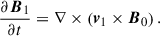
We adopt ideal, gravity-free, pressureless MHD throughout, in which the primitive quantities are the mass density ρ, velocity v, and magnetic field B. We let the subscript 0 denote equilibrium quantities, and consider only static equilibria (v0 = 0). We let (x, y, z) be a Cartesian coordinate system. The equilibrium magnetic field is taken to be uniform and z-directed (B0 = B0ez). We further assume the equilibrium density ρ0 to be a function of x only. The Alfvén speed is defined by vA2 = B02/(μ0ρ0), with μ0 being the magnetic permeability of free space.
We let the subscript 1 denote small-amplitude perturbations. The linearized, time-dependent, ideal MHD equations write
 (1)
(1)
 (2)
(2)
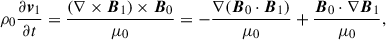
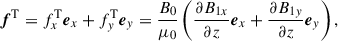
Evidently, the right-hand side (RHS) of Eq. (1) represents the linearized Ampére force, the only restoring force (f) in pressureless MHD. By the second equal sign we show the nominal decomposition of f into the magnetic pressure gradient force (fPG) and magnetic tension force (fT). These further write
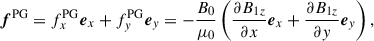 (3)
(3)
 (4)
(4)
where the non-contributing field-aligned components are excluded (see the cylindrical study by Goossens et al. 2009).
We perform classic mode analysis for 3D motions hereafter, kicking off with the Fourier ansatz,
![Mathematical equation: $$ \begin{aligned} g_1 (x, y, z; t) = \mathfrak{R} \{\tilde{g}(x)\exp [-\imath (\omega t- k_y y -k_z z)]\}, \end{aligned} $$](/articles/aa/full_html/2026/03/aa57221-25/aa57221-25-eq5.gif) (5)
(5)
where g1 represents any linear perturbation, with ky (kz) being real-valued out-of-plane (axial) wavenumbers. We see the angular frequency ω as real-valued as well. In component form, Equations (1) and (2) then write
 (6)
(6)
 (7)
(7)
 (8)
(8)
 (9)
(9)
 (10)
(10)
where we adopt the shorthand notation ′ ≔ d/dx. By mode we refer to a nontrivial solution, which is jointly characterized by a mode frequency ω and an eigenvector  . We see the wavenumbers ky and kz as independents, taking equilibrium quantities to be parameters only.
2.2. Fast waves in unbounded uniform media
This subsection examines an unbounded uniform medium for future reference. Now that ρ0 = const, Fourier decomposition is allowed for the x-direction as well, enabling the quantity  in Eq. (5) to be expressible as
 (11)
(11)
Here ğ is a constant. We focus on fast modes, or equivalently compressional Alfvén waves, by assuming ky ≠ 0. Some explicit expressions for the restoring forces readily follow,
 (12)
(12)
where  . It then follows that the parameter
 (13)
(13)
adequately quantifies how one force is related to the other.
Some general properties for fast modes can be readily deduced. To start, the DR reads
 (14)
(14)
where a 3D wavevector k = kxex + kyey + kzez is introduced. Plugging Eq. (14) into Eq. (13) yields that
 (15)
(15)
This means that the magnetic pressure gradient force and the tension force are always in-phase, thereby consistently complementing each other to drive fast motions. Some subtlety arises for near-parallel propagation (kx2 + ky2 ≪ kz2), in which case the tension force dominates such that fast modes become nearly degenerate with shear Alfvén waves. We proceed to define the phase and group velocities as
 (16)
(16)
where ek = k/k. We assume {kx, ky, kz, ω} to be non-negative without loss of generality. The DR (Eq. (14)) then dictates that
 (17)
(17)
namely fast modes are dispersionless. That fast modes are Alfvén-like for near-parallel propagation is reflected in the fact that vgr is largely aligned with the equilibrium field B0 = B0ez.
2.3. Kink modes in slab equilibria
This subsection proceeds to examine a slab equilibrium,
![Mathematical equation: $$ \begin{aligned} \rho _0(x) = \left\{ \!\! \begin{array}{ll} \rho _{\rm i},&|x| < d, \\ [0.2cm] \rho _{\rm e},&|x| > d, \end{array} \right. \end{aligned} $$](/articles/aa/full_html/2026/03/aa57221-25/aa57221-25-eq21.gif) (18)
(18)
where d is the slab half-width. By internal (subscript i) and external (subscript e), we consistently refer to the equilibrium quantities inside and outside the slab, respectively. In particular, the internal (external) Alfvén speed, vAi (vAe), is evaluated with the internal (external) density. We note that a step profile (Eq. (18)) is adopted to avoid the resonant absorption of 3D kink motions in the Alfvén continuum (see Goossens et al. 2011 for conceptual clarifications). We note further that pressureless MHD does not allow slow motions per se. However, we avoid the single use of fast to describe the collective behavior of compressible motions (see Goossens et al. 2009 for more; see also Goossens et al. 2020, 2021). Rather, such terms as B0-straddling or B0-same-side are used to characterize 3D kink motions from the standpoint of group velocities.
We focus on trapped kink modes by supplementing Eqs. (6)–(10) with appropriate boundary conditions (BCs). Only the half volume x ≥ 0 needs to be considered for the resulting boundary value problem (BVP). The BC at the slab axis (x = 0) is specified as  , while all Fourier amplitudes are required to vanish when x → ∞. All mode frequencies are real-valued. Now that the BCs are homogeneous, some straightforward dimensional analysis yields that the mode frequencies can be formally written as
 (19)
(19)
By the second equal sign we recall that the density contrast ρi/ρe is seen as known. The transverse order (j = 1, 2, …) numbers the mode frequencies at a given pair [ky, kz] by increasing order. We follow the convention that the transverse fundamental corresponds to j = 1, while its overtones correspond to j ≥ 2. We detail only the cases j = 1 and j = 2, noting that our analysis readily generalizes to any j. The subscript j is dropped for brevity hereafter, unless confusions may arise.
Some generic properties ensue without solving the BVP. One readily verifies that if ω is a mode frequency for a given pair [ky, kz], then so is −ω. Likewise, if ω is a mode frequency for [ky, kz], then it remains so for the pairs [ − ky, kz], [ky, −kz], and [ − ky, −kz]. It therefore suffices to see ω as positive, and consider only the quadrant ky > 0, kz > 0. Furthermore, Equations (6)–(10) allow the Fourier amplitudes of the restoring forces to be expressed as (see Eqs. (3) and (4))
 (20)
(20)
where  . Equation (20) is formally identical to its counterpart in uniform media (Eq. (12)), the key difference being that the Alfvén speed vA and the quantity Λ need to be discriminated between the interior and exterior. We focus on the interior, supplementing Λ with the subscript i. Evidently,
 (21)
(21)
Some specific results follow from explicit solutions to the BVP. We proceed by defining
 (22)
(22)
 (23)
(23)
 (24)
(24)
We see both me2 and me as positive. The external mode functions therefore write ∝e−mex, meaning that me can be taken as a measure of the capability for slabs to trap kink motions. The signs of κi, e2 and mi2 are unknown at this point. We see kink modes as belonging to the surface (body) subfamily when mi2 > 0 (−ni2 = mi2 < 0), taking mi > 0 (ni > 0) without loss of generality. Trapped 3D kink modes in our slab configuration are known to obey the DR (e.g., Arregui et al. 2007; Yu et al. 2021),
 (25)
(25)
or equivalently
 (26)
(26)
We choose to work with Eq. (25) (Eq. (26)) when handling surface (body) modes. Let k = kyey + kzez. This study pays special attention to both the phase and group velocities as defined by
 (27)
(27)
where ek = k/k.
Of future use is the situation where ky = 0. The DR of 2D kink modes is now textbook material, writing (see Sect. 5.5 in Roberts 2019, and references therein)
 (28)
(28)
Mathematically, Equation (28) can be derived from its 3D counterpart by letting ky = 0. Equation (26) is more appropriate than Eq. (25) for this purpose, because 2D kink modes belong exclusively to the body family. A series of cutoff axial wavenumbers kz(J) are well known to arise,
 (29)
(29)
where J = 1, 2, … in the 2D context. Transverse fundamentals (j = 1) exist for any kz > 0. Taking the first overtone (j = 2) as example, by cutoff we then mean that trapped modes are allowed only when kz > kz(j − 1) = kz(1) (e.g., Nakariakov & Roberts 1995; Li et al. 2013). The solutions to Eq. (28) are denoted by ω2D = ω2D(kz) for clarity. Equation (29) is also involved in our examination of 3D kink modes, which nonetheless require that half integers (J = 1/2, 3/2, …) be addressed.
3. Results
This study is intended to demonstrate how classic mode analysis can be better placed in the context of impulsively excited waves. Regarding the DR (Eq. (25) or equivalently Eq. (26)), it should be ideal that one deduces those generic properties that are insensitive to the density contrast ρi/ρe. However, the transcendental nature of the DR does not allow a completely analytical treatment. We adopt a fixed ρi/ρe = 3, a value relevant for active region loops (e.g., Aschwanden et al. 2004), polar plumes (e.g., Wilhelm et al. 2011), and streamer stalks (e.g., Chen et al. 2011). We solve the DR with standard root-finders for this specific ρi/ρe = 3, and build a more generic picture by proceeding analytically in various limiting cases.
3.1. Generic characterization
This subsection characterizes kink modes by inspecting the form of the DR (Eqs. (25) and (26)). The mode frequencies ω for a given transverse order j then map to a dispersion sheet in the 3D space [ky, kz, ω]. We choose to present a dispersion sheet by showing some of its cuts through constant values of kz. A dispersion curve then results, expressing ω as a function of ky for a given kz. One readily recognizes from Eq. (26) that the surfaces κi2 = 0, κe2 = 0, me = 0, and ni = Jπ (J = 0, 1/2, 1, 3/2, …) are important in organizing the dispersion sheets; these surfaces are where the LHS or RHS of Eq. (26) changes sign. It follows that the intersections of these surfaces are likely to be important as well. In particular, the intersection between the surfaces ni = Jπ and me = 0 satisfies
 (30)
(30)
which defines a set of circles in the ky − kz plane. The reason for kz(J) (see Eq. (29)) to be relevant is then that kz(J) locates where these circles intersect ky = 0. The quantity kz(J) evaluates to
 (31)
(31)
for the chosen ρi/ρe = 3.
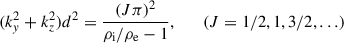
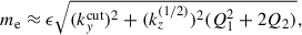
Figure 1 shows a series of ky − ω planes for an increasing sequence of dimensionless axial wavenumbers (kzd) as indicated. The associated mode frequency ω of the transverse fundamental (first overtone) is shown by the black solid (dash-dotted) curve for each kz. A number of curves are further displayed for reference, with the color and linestyle being consistent across all panels. These are also labeled (see Fig. 1c1) to ease our description. Specifically,
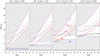 |
Fig. 1. Characterization of trapped 3D kink modes in solar coronal slabs. A density contrast of ρi/ρe = 3 is chosen for illustrative purposes. Plotted in each panel are the dependences on the out-of-plane wavenumber (ky) of the mode frequency of the transverse fundamental (with transverse order j = 1, the black solid curve) and the first overtone (j = 2, black dash-dotted). The hatched portions in any ky − ω plane represent where trapped modes are forbidden, with four curves serving as the relevant borders (labeled in panel c1). Curves 0, 1, 20, and 3 correspond to where |
-
Line 0, the blue solid line, corresponds to κi2 = 0.
-
Line 1, the blue dashed line, corresponds to κe2 = 0.
-
Curve 3, the upper red solid curve, corresponds to me = 0.
-
Curve 20, the lower red solid curve, corresponds to ni = 0.
-
Curves 2Jπ with J = [1/2, 1, 3/2], correspond to ni = Jπ and are shown by the red dotted, dashed, and dash-dotted curves, respectively.
Above all, these curves are important for showing that trapped kink modes are allowed only in the non-hatched portion in a ky − ω plane. The portion bounded by curve 3 from below does not allow trapped modes by definition, given that me2 < 0 therein. That trapped modes are prohibited in the other two hatched portions is because there is always a mismatch between the signs of the LHS and RHS of Eq. (25).
The specific value of kz does not qualitatively impact the transverse fundamental in the following aspects. First, the transverse fundamental is present for any kz > 0 and ky ≥ 0. Second, the fundamental always transitions from a body to a surface type as ky increases, the dividing line being ni = 0 (or equivalently mi2 = 0). Third, the dispersion curve of the fundamental always lies in the horizontal stripe bounded by lines 0 and 1, and is further bounded from above by curve 2π/2 when the fundamental is of the body type. The reason is simply that the LHS of Eq. (25) or Eq. (26) needs to be positive definite.
The behavior of the first overtone may be qualitatively different for different values of kz. This is so despite that the first overtone is always of the body type. Three regimes need to be discriminated regarding how the 2Jπ (with J = 1/2, 1, 3/2) curves are positioned with respect to the stripe between lines 0 and 1.
-
Regime I with 0 < kz < kz(1/2) as typified by Fig. 1a. All three 2Jπ curves lie above the horizontal stripe. One readily verifies that the dispersion curve starts from the intersection between curves 3 and 2π/2, running always between curves 2π and 2π/2. Of relevance is then some cutoff value of ky, only beyond which is the first overtone allowed.
-
Regime II with kz(1/2) < kz < kz(1) as typified by Fig. 1b. Only the 2π/2 curve extends into the horizontal stripe. One readily verifies that the dispersion curve starts from the intersection between curve 3 and line 1. The pair [ky, ω] reads [0, kzvAe] at this intersection, where the transverse overtone is not allowed per se because me = 0. The dispersion curve therefore lies entirely outside the horizontal stripe, running between curves 2π and 2π/2.
-
Regime III with kz > kz(1). Figures 1c1 and 1c2 further typify what happens when kz is below and above kz(3/2), respectively. Curve 2π extends into the horizontal stripe in the former, while curve 23π/2 also does so in the latter. However, the dispersion curve is qualitatively the same in the following sense. One readily verifies that the intersection between curve 2π and line 1 always lies on the dispersion curve, which therefore can be divided into two portions. The portion in the horizontal stripe is always bounded by curve 2π from below, and never touches curve 23π/2 or line 1. On the other hand, the portion outside the horizontal stripe always runs between curves 2π and 2π/2.
All these properties follow from the inspection of the signs of the LHS and RHS of Eq. (26). Similar conclusions can therefore be inferred for overtones of higher transverse order (j). All overtones belong exclusively to the body type, even though some quantitative difference from the first overtone does arise for j ≥ 3 regarding how the associated dispersion curve is positioned in the ky − ω plane. We take the second overtone j = 3 for instance, and by difference we mean that curves 2Jπ with J = 3/2, 2, 5/2 are relevant simply because the cot function is π-periodic.
3.2. Transverse fundamental
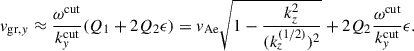
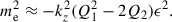
This subsection is devoted to the transverse fundamental. Figure 2 displays the distribution in the ky − kz plane of the phase speed as equally spaced contours. Also plotted are the filled contours of the parameter ni, to evaluate which we now see ω in Eq. (24) as the mode frequency. We note that ni makes sense only for body modes (ni2 > 0), meaning that the portion not occupied by the color map corresponds to surface modes. Figure 3 further plots how the y-component (vgr, y, black contours) and z-component (vgr, z, red) of the group velocity depend on [ky, kz].
 |
Fig. 2. Transverse fundamental kink mode in a coronal slab with a density contrast ρi/ρe = 3. The dependence on [ky, kz] of the phase speed |

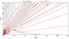 |
Fig. 3. Transverse fundamental kink mode in a coronal slab with a density contrast ρi/ρe = 3. Shown are the dependences on [ky, kz] of the y-component (the black contours) and the z-component (red) of the group velocity. All contours are equally spaced. |
Some analytical progress can be made to help digest Figs. 2 and 3. Consider near-parallel propagation first (ky2 ≪ kz2), and start with the particular case ky = 0. It is well documented for these 2D modes (e.g., Roberts 2019, Chapter 5) that the phase speed ω2D(kz)/kz decreases monotonically with kz, approaching vAe (vAi) when kzd → 0 (kzd → ∞). This behavior is what one sees along ky = 0 in Fig. 2. One further deduces that
 (32)
(32)
 (33)
(33)
by specializing Eqs. (18) and (16) in Li et al. (2013) to pressureless MHD. We note that ni evaluates to  for 2D modes, and is itself a monotonically increasing function of kz (see Fig. 2). Equations (32) and (33) then help show that nid → 0 for kzd → 0 and nid → π/2 when kzd → ∞.
We now consider the situation 0 < ky2/kz2 ≪ 1. It follows from Li et al. (2023, Eq. (9)) that
![Mathematical equation: $$ \begin{aligned} \omega (k_y, k_z) \approx \omega ^\mathrm{2D} \left[1+\dfrac{1}{2} \dfrac{m_{\rm e}^\mathrm{2D} d -1}{(k_z d)^2 + (m_{\rm e}^\mathrm{2D} d)(\omega ^\mathrm{2D} d/v_{\rm Ai})^2} (k_y d)^2 \right], \end{aligned} $$](/articles/aa/full_html/2026/03/aa57221-25/aa57221-25-eq42.gif) (34)
(34)
where ω2D = ω2D(kz) and  . Equation (34) explicitly shows that the correction to ω2D is only quadratic in ky, meaning that vgr, y = ∂ω/∂ky → 0 when kyd → 0 (see Fig. 3). More importantly, one notices from Eqs. (32) and (33) that
  for kzd ≪ 1 and
  for kzd ≫ 1. Overall,
  turns out to be a monotonically increasing function of kz. One then recognizes the existence of some critical axial wavenumber kz2D, c, which renders
  negative (positive) when kz < kz2D, c (kz > kz2D, c). We let 𝒞 denote the coefficient in front of (kyd)2 in Eq. (34). It then follows that 𝒞 reverses its sign when kzd passes through kz2D, cd. Somehow Fig. 2 indicates that both vph and ni tend to decrease with ky at any given kz, demonstrating no signature of kz2D, cd. This behavior can be explained by Eqs. (27) and (24) where vph and ni are defined; the direct ky-dependences tend to dominate the indirect ky-dependences through ω. However, kz2D, cd plays an important role for vgr, y and vgr, z. One sees that vgr, y tends to decrease to negative values with increasing ky for small kz, whereas vgr, y increases to positive values when ky increases from zero for large kz. This is a direct consequence of Eq. (34), which actually helps one to deduce kz2D, cd ≈ 1.38 from Fig. 3 by locating where vgr, y changes sign for ky → 0. The quantity kz2D, c is relevant for vgr, z as well, to show which we focus on the range kz < kz2D, c. One sees that vgr, z tends to decrease (increase) with ky when kz is fixed at some small (large) value. This is readily understandable if one notices the relevance of d𝒞/dkz when evaluating ∂ω/∂kz with Eq. (34).
We now address the situation ky2/kz2 ≫ 1 where sufficiently oblique modes can be safely taken as surface modes. It is known that (Tatsuno & Wakatani 1998; Yu et al. 2021)
 (35)
(35)
approximately solves Eq. (25). The more restrictive situation kyd → ∞ is well studied, yielding  (e.g., Ionson 1978; Goossens et al. 1992; Ruderman et al. 1995). One sees from Fig. 2 that the contours of the phase speed vph largely become radially directed in the ky − kz plane. This behavior can be explained by the simplest approximation ω ≈ kzCkink, which yields that
 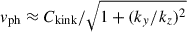 . Furthermore, this simplest approximation also helps understand the overall tendencies for vgr, y to be small and for vgr, z to approach Ckink when ky2/kz2 ≫ 1 (see Fig. 3). However, some subtlety remains regarding the ky-dependence of vgr, y or vgr, z even if the improved approximation (Eq. (35)) is employed. For instance, one expects with Eq. (35) that vgr, y approaches zero from below given that C(ky) decreases monotonically with ky. Figure 3, however, indicates that vgr, y > 0 for sufficiently large ky. Likewise, Eq. (35) suggests that vgr, z should approach Ckink from above. This contradicts the behavior of vgr, z at large ky. It turns out that Eq. (35) needs to be improved to address the ky-dependence for those ranges of ky where tanh(kyd) varies only slowly. Writing
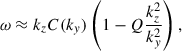 (36)
(36)
we proceed to Taylor-expand all terms on both sides of the DR (Eq. (25)) to the lowest order in kz2/ky2. The coefficient Q then results from some algebra, reading
![Mathematical equation: $$ \begin{aligned} Q = \dfrac{1}{4} \dfrac{(1-\rho _{\rm e}/\rho _{\rm i})^2}{[\rho _{\rm e}/\rho _{\rm i}+\tanh (k_y d)]^2} \left\{ \tanh (k_y d) - (k_y d)[1-\tanh (k_y d)] \right\} . \end{aligned} $$](/articles/aa/full_html/2026/03/aa57221-25/aa57221-25-eq52.gif) (37)
(37)
For the chosen ρi/ρe = 3, Equation (36) proves to be remarkably accurate when ky/kz ≳ 2. Consequently, one readily explains the large-ky behavior of vgr, y or vgr, z by noting that
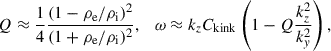 (38a)
(38a)
 (38b)
(38b)
for sufficiently large kyd.
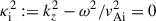
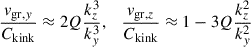
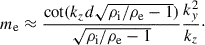
Figure 4 gathers the directional information of the group (vgr) and phase velocities (vph), aiming to categorize transverse fundamental kink modes on the ky − kz plane. Plotted are the [ky, kz]-dependences of (a) the angle (∠(vgr, ez)) between vgr and the z-direction, and (b) the angle (∠(vgr, vph) between the two vector velocities themselves. The angles are measured counterclockwise from vgr, the readings being in degrees. All contours are equally spaced. Also shown by the filled contours is the parameter Λi, which is recalled to be the ratio of the magnetic pressure gradient force to the magnetic tension force (see Eq. (21)).
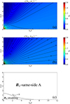 |
Fig. 4. Transverse fundamental kink mode in a coronal slab with a density contrast ρi/ρe = 3. Shown are the dependences on [ky, kz] of (a) the angle between the group velocity vgr and the z-direction, and (b) the angle between the group velocity vgr and the phase velocity vph. The angles are in degrees and measured counterclockwise from vgr to |

We consider the quantity Λi first. By definition, Λi is positive definite for the transverse fundamental and overtones alike, given that all trapped modes ensure κi2 = kz2 − ω2/vAi2 < 0 (see Fig. 1). Figure 4a further indicates that Λi tends to be smaller than unity for the majority of the [ky, kz] combinations, with the portion Λi > 1 restricted to the lower left corner. This can be understood with the approximate expressions that were presented previously. The expressions for 2D modes (ky = 0, Eqs. (32) and (33)) suggest that Λi → ρi/ρe − 1 when kzd ≪ 1 and Λi → 0 when when kzd → ∞. Addressing a small ky2/kz2, Equation (34) further suggests that Λi decreases (increases) with ky for relatively small (large) values of kz that ensure a negative (positive) ky2-correction. Likewise, one deduces from Eq. (36) that
 (39)
(39)
when ky2/kz2 → ∞. Actually, one sees from Fig. 4a that Λi is nearly uniform for sufficiently large ky; the subtle ky− (and kz-) dependences of C(ky) and the Q term play only a marginal role in determining the gross distribution of Λi.
We now attempt to place the angle distributions in the context of Λi. For immediate future reference, we classify trapped 3D kink modes into the following three regimes, noting that vgr, z is positive definite in our context.
-
B0-straddling, by which we mean the situation where vgr, y < 0 (i.e., vgr and vph straddle B0).
-
B0-same-side A, by which we mean the situation where vgr, y > 0 and |∠(vgr, ez)| < 15°.
-
B0-same-side F, by which we refer to the situation where vgr, y > 0, |∠(vgr, ez|> 15°, and |∠(vgr, vph)| < 15°.
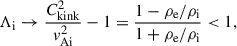
We note that by B0-same-side we mean vgr and vph sit on the same side of B0. This classification scheme largely comes from the analogy with 3D waves (ky > 0) in unbounded uniform media (see Sect. 2.2), with the threshold angle arbitrarily chosen to be some small value (15° here). We note that the waves examined in Sect. 2.2, broadly called fast therein, need to be categorized into the B0-same-side A and B0-same-side F subgroups here. Equation (15) then offers an unambiguous association of this categorization with the force ratio; the B0-same-side A subgroup arises when the force ratio Λ < tan2(15° ) ≈ 0.07, whereas the B0-same-side F subgroup arises when the opposite is true. The letters A and F are meant to distinguish the Alfvén-like modes and the genuinely fast-like modes. The B0-straddling subgroup is absent in Sect. 2.2, but bears substantial resemblance to slow waves in unbounded uniform media with non-vanishing puressue (e.g., Roberts 2019, Sect. 2.7). Figures 4a and 4b indicate that transverse fundamental kink modes qualify as B0-same-side A in the majority of the ky − kz plane. This is true even for highly oblique propagation (ky2/kz2 ≫ 1), despite that the force ratio Λi is only marginally small (1/2 for the chosen ρi/ρe = 3, see Eq. (39)). In this regard, our classification scheme agrees with the force-ratio-based argument by Goossens et al. (2009) in that transverse fundamental kink modes are largely Alfvén-like, despite that cylindrical geometry was examined therein. More striking is the B0-straddling subgroup, which shows up at the lower left corner in the ky − kz plane. By striking we mean that pressureless MHD does not allow slow waves in textbook sense as far as unbounded uniform media are concerned. However, these motions do make it into Fig. 4, thereby highlighting the intricacies that transverse structuring brings into wave studies. For clarity, we collect our classification in Fig. 4c and label the subgroups accordingly. One sees that the force ratio Λi ≳ 1 in the B0-straddling corner.
3.3. First transverse overtone
This subsection is devoted to the first transverse overtone. Figure 5 follows the format of Fig. 2 to present the [ky, kz]-dependences of the phase speed vph and the quantity ni. We note that trapped 3D modes are forbidden within the circle  , which reads 1.11 given a ρi/ρe = 3. We note also that trapped 2D modes (ky = 0) are further prohibited for kz(1/2) < k < kz(1) = 2kz(1/2). When allowed, trapped modes belong exclusively to the body type (ni2 > 0), meaning that ni makes sense. Figure 6 presents, in a form identical to Fig. 3, the distributions in the ky − kz plane of the y component (vgr, y) and z-component (vgr, z) of the group velocity.
 |
Fig. 5. Similar to Fig. 2, but for the first transverse overtone. Trapped 3D modes are forbidden within the circle |
It proves convenient to make analytical progress in various limiting cases to help understand Figs. 5 and 6. First consider highly oblique propagation ky2/kz2 ≫ 1. One readily sees from the DR (Eq. (26)) that ni → π− when ky2/kz2 → ∞, meaning that the leading order solution  reads
reads
 (40)
(40)
It then follows that  is approximately proportional to
 ![Mathematical equation: $ \sqrt{1+\pi^2/[(k_y d)^2+(k_z d)^2]} $](/articles/aa/full_html/2026/03/aa57221-25/aa57221-25-eq62.gif) , meaning that the contours of vph eventually become a series of circles centered at the origin on the ky − kz plane. This is what one sees from Fig. 5. Furthermore, Equation (40) indicates that
, meaning that the contours of vph eventually become a series of circles centered at the origin on the ky − kz plane. This is what one sees from Fig. 5. Furthermore, Equation (40) indicates that
![Mathematical equation: $$ \begin{aligned} \dfrac{v_{\mathrm{gr},y}}{v_{\rm Ai}} \approx \dfrac{1}{\sqrt{1+[\pi ^2+(k_z d)^2]/(k_y d)^2}}\cdot \end{aligned} $$](/articles/aa/full_html/2026/03/aa57221-25/aa57221-25-eq63.gif) (41)
(41)
At a given kz, this means that vgr, y approaches the internal Alfvén speed vAi as a monotonically increasing function of ky, in close agreement with Fig. 6. Likewise, one sees from Eq. (40) that
![Mathematical equation: $$ \begin{aligned} \dfrac{v_{\mathrm{gr},z}}{v_{\rm Ai}} \approx \dfrac{1}{\sqrt{1+[\pi ^2+(k_y d)^2]/(k_z d)^2}}, \end{aligned} $$](/articles/aa/full_html/2026/03/aa57221-25/aa57221-25-eq64.gif) (42)
(42)
which further simplifies to  when (kyd)2 ≫ π2. This means that the contours of vgr, z eventually become a series of rays radially directed from the origin on the ky − kz plane, thereby explaining the red contours for ky2/kz2 ≫ 1 in Fig. 6. For completeness, we note that an improved version of Eq. (40) can be readily derived by writing
 (43)
(43)
with  seen as a small parameter. Expanding both sides of Eq. (26), one readily verifies that the ϵ-corrections start with third order in the parentheses of Eq. (43). An approximate solution that corrects
  to forth order reads
![Mathematical equation: $$ \begin{aligned} \omega (k_y, k_z) \approx \hat{\omega } \left[ 1 - \dfrac{Q_3}{(\hat{\omega } d/v_{\rm Ai})^3} + \dfrac{Q_4}{(\hat{\omega } d/v_{\rm Ai})^4} \right], \end{aligned} $$](/articles/aa/full_html/2026/03/aa57221-25/aa57221-25-eq69.gif) (44)
(44)
where
 (45a)
(45a)
 (45b)
(45b)
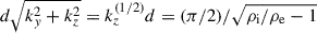
We now consider small values of kyd. Some subtlety arises regarding what small means given the zone where trapped modes are forbidden. Three cases need to be discriminated in terms of kz. We start with Case I where  . As indicated by Fig. 1a, the dispersion curve in this case starts from the intersection (P) between the curves me = 0 and ni = π/2 therein. See kz as given, and let the coordinates of P be denoted by [kycut, ωcut]. One finds with the definitions of me and ni (Eqs. (23) and (24)) that
![Mathematical equation: $$ \begin{aligned} k_y^\mathrm{cut}&= \sqrt{[k_z^{(1/2)}]^2 - k_z^2}, \end{aligned} $$](/articles/aa/full_html/2026/03/aa57221-25/aa57221-25-eq73.gif) (46a)
(46a)
 (46b)
(46b)
Evidently, kycut is some critical out-of-plane wavenumber, only beyond which trapped 3D modes are allowed for a given kz. Defining a small parameter 0 < ϵ ≪ 1 as
 (47)
(47)
we proceed to examine how trapped modes behave in the immediate vicinity of the forbidden zone by writing
![Mathematical equation: $$ \begin{aligned} \omega (k_y, k_z) = \omega ^\mathrm{cut} \left[ 1 + Q_1 \epsilon + Q_2 \epsilon ^2 + \ldots \right]. \end{aligned} $$](/articles/aa/full_html/2026/03/aa57221-25/aa57221-25-eq76.gif) (48)
(48)
Some tedious algebra yields that
 (49a)
(49a)
![Mathematical equation: $$ \begin{aligned} Q_2&= \dfrac{1}{2(k_z^{(1/2)} d)^2} \left[1 -\dfrac{k_z^2}{(k_z^{(1/2)})^2} \right] \nonumber \\&\quad \left\{ (k_z d)^2 - \left(\dfrac{\pi }{2}\right)^4 \dfrac{[1 -k_z^2/(k_z^{(1/2)})^2]^3}{[\rho _{\rm i}/\rho _{\rm e} -k_z^2/(k_z^{(1/2)})^2]^2} \right\} . \end{aligned} $$](/articles/aa/full_html/2026/03/aa57221-25/aa57221-25-eq78.gif) (49b)
(49b)
Evidently, both Q1 and Q2 approach zero when kz → kz(1/2), meaning that the expansion (48) is of little use therein. Furthermore, Q2 is a bit intricate in that it switches from negative to positive values when kz increases through some critical value. Regardless, both Q1 and Q2 are involved in the approximate expression for me,
 (50)
(50)
thereby providing a direct measure of the trapping capability of the slab when ky deviates slightly from kycut.
Equation (48) proves largely adequate for explaining Figs. 5 and 6, provided that kz is not that close to kz(1/2). We take the ni distribution in Fig. 5 for instance. One finds from Eq. (48) that
![Mathematical equation: $$ \begin{aligned} n_{\rm i} \approx \dfrac{\pi }{2} \left[1+ \dfrac{(k_y^\mathrm{cut})^2}{(k_z^{(1/2)})^2} \epsilon \right], \end{aligned} $$](/articles/aa/full_html/2026/03/aa57221-25/aa57221-25-eq80.gif) (51)
(51)
suggesting that ni − π/2 scales largely as ∝ϵ when ky deviates slightly from kycut for a given kz. One further finds that
![Mathematical equation: $$ \begin{aligned} v_{\rm ph} \approx v_{\rm Ae} \left[1+\dfrac{Q_1^2 + 2 Q_2 - Q_1}{2} \epsilon ^2 \right]. \end{aligned} $$](/articles/aa/full_html/2026/03/aa57221-25/aa57221-25-eq81.gif) (52)
(52)
The phase speed vph therefore tends to decrease from the external Alfvén speed at a rather slow rate (∝ϵ2). Now consider Fig. 6. It follows from Eq. (48) that
 (53)
(53)
It immediately follows that vgr, y decreases from vAe toward zero when kz increases from zero toward kz(1/2) along the outer edge of the forbidden zone. Furthermore, that Q2 changes sign means that vgr, y decreases (increases) from the edge value when ky increases from kycut for a given kz that is below (above) some critical value. Equation (48) can also be used to derive an approximate expression for vgr, z. This derivation is somehow complicated by the kz-dependences of kycut and ϵ (see Eqs. (46) and (47)). Some algebra yields that
![Mathematical equation: $$ \begin{aligned} v_{\mathrm{gr},z} \approx v_{\rm Ae} \dfrac{k_z}{k_z^{(1/2)}} \left[ 1+\left( -1 + 2Q_2 \dfrac{(k_z^{(1/2)})^2}{(k_y^\mathrm{cut})^2} \right)\epsilon \right]. \end{aligned} $$](/articles/aa/full_html/2026/03/aa57221-25/aa57221-25-eq83.gif) (54)
(54)
Taking ϵ → 0, one deduces from Eq. (54) that vgr, z varies from zero toward vAe when kz is surveyed along the edge of the forbidden zone from zero toward kz(1/2). The ϵ-correction, one the other hand, immediately suggests that vgr, z decreases from its edge value when ky increases from kycut for a kz ensuring Q2 < 0. This is in agreement with Fig. 6. Somehow puzzling is that the same ky-dependence actually persists for those kz that yield positive Q2. This can be addressed by expanding the Q2-term in Eq. (54) with the aid of Eq. (49), the result being
![Mathematical equation: $$ \begin{aligned} 2Q_2 \dfrac{(k_z^{(1/2)})^2}{(k_y^\mathrm{cut})^2} = \dfrac{1}{(k_z^{(1/2)} d)^2} \left\{ (k_z d)^2 - \left(\dfrac{\pi }{2}\right)^4 \dfrac{[1 -k_z^2/(k_z^{(1/2)})^2]^3}{[\rho _{\rm i}/\rho _{\rm e} -k_z^2/(k_z^{(1/2)})^2]^2} \right\} . \end{aligned} $$](/articles/aa/full_html/2026/03/aa57221-25/aa57221-25-eq84.gif) (55)
(55)
Evidently, this Q2-term is consistently smaller than unity. It then follows that the coefficient of ϵ in Eq. (54) is always negative.
We now move on to Case II where  . This case is somehow peculiar in that there exist no trapped 2D modes (ky = 0), whereas trapped 3D modes suddenly arise when ky becomes finite, regardless of how small kyd is. One readily verifies that me → 0 when ky → 0, meaning that the leading-order solution to Eq. (26) reads ω ≈ kzvAe. Defining ϵ = ky2/kz2 ≪ 1, we look for improved approximate solutions in the form ω = kzvAe(1 + Q1ϵ − Q2ϵ2 + …), or equivalently
![Mathematical equation: $$ \begin{aligned} \omega (k_y, k_z) \approx k_z v_{\rm Ae} \left[ 1 + Q_1 \dfrac{k_y^2}{k_z^2} - Q_2 \dfrac{k_y^4}{k_z^4} + \ldots \right]. \end{aligned} $$](/articles/aa/full_html/2026/03/aa57221-25/aa57221-25-eq86.gif) (56)
(56)
Some algebra yields that
![Mathematical equation: $$ \begin{aligned} Q_1 = \dfrac{1}{2}, \qquad Q_2 = \dfrac{1}{2} \left[ \dfrac{1}{4} +\dfrac{\cot ^2(k_z d \sqrt{\rho _{\rm i}/\rho _{\rm e}-1})}{\rho _{\rm i}/\rho _{\rm e}-1} \right]. \end{aligned} $$](/articles/aa/full_html/2026/03/aa57221-25/aa57221-25-eq87.gif) (57)
(57)
The reason for us to retain the Q2 term is that it is involved in me2, which approximates to
More specifically, one finds that
 (58)
(58)
For a fixed kz, the slab therefore possesses some poorer trapping capability (me ∝ ky2) than in Case I where  (Eq. (50)). More importantly, that me possesses a continuous ky-dependence means that the sudden appearance of trapped 3D modes for ky > 0 does not result in any abrupt change in the the temporal response of the slab to impulsive, localized, 3D drivers.
Equation (56) proves adequate for explaining some key features of Figs. 5 and 6. One deduces from Eq. (56) that
 (59)
(59)
When ky → 0, the quantity ni therefore increases monotonically from π/2 to π as kz increases from kz(1/2) to kz(1). The contours of ni for small ky, on the other hand, are expected to be concentric circles as indeed seen in Fig. 5. One further deduces that
![Mathematical equation: $$ \begin{aligned} v_{\rm ph} \approx v_{\rm Ae} \left[1- \dfrac{1}{2} \dfrac{\cot ^2(k_z d \sqrt{\rho _{\rm i}/\rho _{\rm e}-1})}{(\rho _{\rm i}/\rho _{\rm e}-1)} \dfrac{k_y^4}{k_z^4} \right], \end{aligned} $$](/articles/aa/full_html/2026/03/aa57221-25/aa57221-25-eq92.gif) (60)
(60)
meaning that vph decreases from vAe at a very slow rate (∝ky4) when ky increases for a given kz. We now move on to Fig. 6, to explain which it suffices to retain only the Q1 term in Eq. (56). One finds that
 (61)
(61)
thereby explaining why the vgr, y contours are largely radially directed. One further finds that
 (62)
(62)
meaning that vgr, z for a given kz tends to decrease rather slowly with ky. Equation (62) also explains why the vgr, z contours are largely radially aligned when kz is not that close to kz(1).
We now address Case III where kz > kz(1). It is textbook material that trapped 2D modes (ky = 0) are now allowed, their phase speeds ω2D(kz)/kz decreasing monotonically from vAe to vAi when kz increases from kz(1) to large values (e.g., Roberts 2019, Chapter 5). One further finds that
![Mathematical equation: $$ \begin{aligned} \omega ^\mathrm{2D}(k_z) \approx k_z v_{\rm Ae} \left[ 1-\dfrac{(\rho _{\rm i}/\rho _{\rm e}-1)\pi ^2}{2} \left(\dfrac{k_z}{k_z^{(1)}}-1\right)^2 \right] \end{aligned} $$](/articles/aa/full_html/2026/03/aa57221-25/aa57221-25-eq95.gif) (63)
(63)
when kz exceeds kz(1) only marginally. A similar expression is available for trapped 2D sausage modes (Li et al. 2018, Eq. (22)), and Eq. (63) can be derived with the same procedure therein. Likewise, one finds that
 (64)
(64)
by specializing Eq. (16) in Li et al. (2013) to the pressureless limit. We note that the quantity  for trapped 2D overtones behaves similarly to transverse fundamentals in that ni also increases monotonically with kz (see Fig. 5). Equations (63) and (64) help explicitly show that nid → π when kz → kz(1) and nid → 3π/2 when kzd → ∞.
We now consider what happens when 0 < ky2/kz2 ≪ 1. One readily verifies that Eq. (34) holds for transverse overtones as well, as long as the quantities ω2D and  are interpreted appropriately. We rewrite Eq. (34) as
![Mathematical equation: $$ \begin{aligned} \omega (k_y, k_z) \approx \omega ^\mathrm{2D}(k_z) [1+ \mathcal{C} (k_z) (k_y d)^2] \end{aligned} $$](/articles/aa/full_html/2026/03/aa57221-25/aa57221-25-eq99.gif) (65)
(65)
for the ease of description. It follows from Eqs. (63) and (64) that 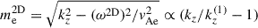 when kz barely exceeds kz(1), while
  when kzd ≫ 1. The quantity
  itself turns out to be a monotonically increasing function of kz. Equation (34) then indicates that there must exist some critical axial wavenumber, kz2D, c, such that 𝒞 < 0 (𝒞 > 0) when kz(1) < kz < kz2D, c (kz > kz2D, c). One therefore deduces from Eq. (65) that vgr, y = ∂ω/∂ky varies from zero when ky → 0 toward negative (positive) values for those values of kz that ensure 𝒞 < 0 (𝒞 > 0). This is what one sees from Fig. 6, and the vgr, y = 0 contour therein actually identifies kz2D, cd ≈ 2.74 for the chosen ρi/ρe = 3. We restrict ourselves to kz(1) < kz < kz2D, c. Figure 6 shows the subtle feature that vgr, z tends to decrease (increase) from its edge value (kz → 0) when ky increases for relatively small (large) values of kz. This can be adequately addressed by taking the kz-derivative of Eq. (65), even though the cumbersome d𝒞/dkz term somehow complicates the matter.
Figure 7 applies the same format of Fig. 4 and the associated classification scheme to the first transverse overtone. We note that the filled contours display only a limited range for the force ratio Λi, despite that Λi can be evaluated wherever trapped modes are permitted. Consider trapped 2D modes first (ky = 0), which are recalled to arise for kz > kz(1). One readily finds from Eqs. (63) and (64) that Λi → ρi/ρe − 1 when kz approaches kz(1) from above, and Λi → 0 when kzd → ∞. For highly oblique propagation (ky2/kz2 ≫ 1), however, Equation (44) suggests that Λi = ω2/kz2vAi2 − 1 approximates to [π2 + (kyd)2)]/(kzd)2 and may therefore take extremely large values.
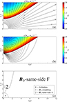 |
Fig. 7. Similar to Fig. 4, but for the first transverse overtone. Only a limited range is plotted for the quantity Λi because Λi takes up too diverse a range. Panel c overviews how the overtone behaves on the ky − kz plane. Trapped 3D modes are forbidden where |

Figure 7c overviews how the first overtone behaves on the ky − kz plane. The disc 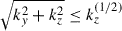 , labeled 0, is recalled to be where trapped 3D modes are forbidden. Our classification scheme is then applied, and all the three subgroups are now relevant. The B0-straddling subgroup (with vgr, y < 0, labeled 1) remains associated with force ratios Λi ≳ 1, despite that this subgroup is restricted to a substantially smaller portion when compared with the fundamental. The B0-same-side F subgroup corresponds to the vast portion to the right of the |∠(vgr, ez)| = 15° contour. Our additional criterion |∠(vgr, vph)| < 15° does not provide further constraints per se. In fact, Figure 7b indicates a small ∠(vgr, vph) almost everywhere, which is particularly true for oblique propagation (ky2/kz2 ≫ 1). This feature, in conjunction with the overall tendency for Λi to be (relatively) large, means that the B0-same-side F subgroup somehow closely resembles what happens in unbounded uniform media. However, the B0-same-side A subgroup deviates considerably from its counterpart in an unbounded uniform medium, in which case one recalls a Λ ≲ 0.07. The force ratio Λi for the B0-same-side A subgroup here, in contrast, may readily exceed ρi/ρe − 1. We note that |∠(vgr, ez)| evaluates to 45° when Λ = 1 in an unbounded uniform medium (see Eq. (15)). Our specific threshold of 15° for mode categorization is therefore only for illustrative purposes. A larger threshold (up to 45°) does not impact the categorization of the transverse fundamental, given that |∠(vgr, ez)| does not exceed ∼11° (Fig. 4). Nonetheless, a larger threshold will broaden the ky − kz portion where the first overtone qualifies as B0-same-side A in Fig. 7c. The rest of the B0-same-side portion always qualifies as B0-same-side F modes; |∠(vgr, vph)| is consistently smaller than ∼15° and therefore not a discriminating factor. Importantly, the threshold angle is not involved hereafter; only the distinction between B0-straddling and B0-same-side is employed.
4. Implications for impulsively excited 3D kink motions
The question arises of how the above-presented mode analysis connects to the spatio-temporal evolution of a density-enhanced slab in response to localized initial exciters. We start by noting that the problem at hand is an initial value problem (IVP) governed by the time-dependent MHD Equations (1) and (2) over the infinite [x, y, z]-volume. Conceptually, the nominal boundaries x, y, z → ±∞ need to be such that no boundary conditions (BCs) are specified or equivalently that the dependent variables do not diverge (see, e.g., Gao et al. 2024, and references therein). The most unambiguous way to specify initial exciters, on the other hand, is to perturb the velocities only (v1(x, y, z, t = 0)≠0, B1(x, y, z, t = 0) = 0; see Sect. 6.1.2 in Goedbloed et al. 2019). We proceed with the following assumptions for definitiveness. First, the only non-vanishing independent quantity at t = 0 is v1x. Second, v1x(x, y, z, t = 0) is even in x to ensure kink parity, and is even in both y and z as well. Third, the implementation of v1x(x, y, z, t = 0) is such that one needs only to consider the range of [ky, kz] examined in Figs. 3 and 6.
Quantitative progress can be made by presenting the formal solution to the IVP (Li et al. 2023),
![Mathematical equation: $$ \begin{aligned}&v_{1x}(x,y,z,t) = \int _{-\infty }^{\infty } \mathrm{d} k_y \int _{-\infty }^{\infty } \mathrm{d} k_z \nonumber \\&\quad \left\{ \sum _j \left[\mathcal{F} _j(x; k_y, k_z) \mathrm{e}^{\imath (\omega _j t - k_y y - k_z z)} \right] +\text{ improper} \right\} . \end{aligned} $$](/articles/aa/full_html/2026/03/aa57221-25/aa57221-25-eq105.gif) (66)
(66)
Equation (66) is so written by following the approach of Fourier integrals (e.g., Oliver et al. 2014, 2015) or equivalently the idea of decomposing the time-dependent wave fields into the eigenmodes of the MHD force operator (e.g., Li et al. 2022; Wang et al. 2023). We adopt the nomenclature of the latter. The decomposition in the y- or z-direction is self-evident, and one then ends up with an eigenvalue problem with x being the only independent variable and [ky, kz] serving as parameters. At any given pair [ky, kz], the eigenspectrum of the MHD force operator for our slab equilibrium comprises two subspectra. The point subspectrum is populated by a finite number of eigensolutions, which are labeled by j and are equivalent to our trapped modes (me2 > 0). By construction, ωj = ωj(ky, kz) is dictated by the DR. The other subspectrum (with me2 < 0), called improper continuum, comprises those eigensolutions whose eigenfrequencies continuously cover the range from some critical frequency out to infinity. This improper continuum arises in our context as a result of the physical requirement that no BCs should be specified at x → ±∞. Regardless, the contribution from the continuum eigenmodes (labeled “improper” in Eq. (66)) attenuates rapidly with time and hence are not of further interest here.
What survives at large times is the contribution from trapped modes. We focus on the slab axis x = 0, supposing further that only the transverse fundamental and its first overtone are relevant. These simplifications suffice to illustrate both the usefulness of and intricacies in the MSP that we adopt to digest the morphological features of wave propagation. Suppose that the MSP applies to some [y, z, t] or more appropriately to some [y/t, z/t] with [y, z, t] seen as given. Equation (66), while nominally involving all [ky, kz], is actually dominated only by a series of narrow regions (or wavepackets in physical terms) on the ky − kz plane. Let wavepackets (WPs) be numbered by n and represented by the central wavenumbers [Kn, y, Kn, z]. It follows from the general theory of the MSP that (e.g., Whitham 1974, Chapter 11)
![Mathematical equation: $$ \begin{aligned} v_{1x}(x=0, y, z, t) \sim t^{-1} \sum _n \left[\mathcal{G} _n(K_{n, y}, K_{n, z}) \mathrm{e}^{\imath (\omega _n t - K_{n, y} y - K_{n, z} z)} \right], \end{aligned} $$](/articles/aa/full_html/2026/03/aa57221-25/aa57221-25-eq106.gif) (67)
(67)
where ωn = ωn(Kn, y, Kn, z) is given by the DR. Involved in the summation is any WP that solves the kinematic equation
 (68)
(68)
It suffices to consider only the first quadrant (y, z > 0) given the assumed y- and z-symmetries of the exciter v1x(x, y, z, t = 0). Some subtlety arises now in that so far our mode analysis addresses only the first quadrant in the wavenumber plane (ky > 0, kz > 0), with vgr, y < 0 for our B0-straddling modes. WPs associated with these B0-straddling modes remain possible to show up for [y > 0, z > 0]. Suppose that some [K′n, y > 0, K′n, z > 0] satisfies

The symmetry discussions on Eq. (19) then dictate that WP [Kn, y = −K′n, y, Kn, z = K′n, z] solves Eq. (68).
Figure 8 collects the results of our mode analysis to show what WPs are expected in different portions of the y/t − z/t plane. The horizontal and vertical axes are not to the same scale, otherwise Fig. 8 would be difficult to present. Different portions are discriminated by the different straight lines, whose slopes (S > 0) are determined by Eq. (68). Specifically,
 |
Fig. 8. Categorization of the y/t − z/t plane in terms of large-time expectations for the morphological features of impulsive kink motions. The bordering straight lines are determined by the limiting behavior of the group velocities as derived from Figs. 3 and 6. Line I+ pertains to B0-same-side fundamental modes, while line I− (II−) pertains to B0-straddling modes associated with the transverse fundamental (first overtone). Four sectors result. Different morphological features are expected for different sectors, the difference being particularly pronounced when line I− is crossed. One representative point in each sector (marked P1 to P4) is selected for further quantitative analysis (see text for more details). |
-
the slope of line II− reads SII− = 50.6, the minimal |vgr, z/vgr, y| that B0-straddling overtone modes may reach.
-
the slope of line I− reads SI− = 7.6, the minimal |vgr, z/vgr, y| that B0-straddling fundamental modes may reach.
-
the slope of line I+ reads SI+ = 4.9, the minimal vgr, z/vgr, y reachable by B0-same-side fundamental modes.
Four sectors are eventually discriminated, with Eq. (68) determining the types of WPs that each sector allows. One way to visualize this is that Fig. 8 is superimposed by all pairs of [vgr, y, vgr, z] in Figs. 3 and 6, with the sign of vgr, y reversed for B0-straddling modes. Overall, two clouds show up, one for the transverse fundamental and the other for its first overtone. Wave signatures can be found only in these clouds, if one sees t in Eq. (68) as some given large time and therefore translates the y/t − z/t plane into the more intuitive y − z plane. We choose not to do this because the resulting figure is way too crowded. Rather, we somehow arbitrarily choose one space-time point from the cloud(s) within each sector in Fig. 8. The coordinates [y/t, z/t] of these points, labeled P1 to P4, are then inverted with Eq. (68) for the allowed WPs. Table 1 then results, where the third and fourth columns present the central wavenumbers of the inverted WPs from the fundamental and first overtone, respectively.
Wavepackets for a representative set of space-time points.
Some key morphological features at some arbitrarily given large t can be predicted for wave propagation in the first quadrant (y, z > 0) of the x = 0 plane. We focus on the wavefronts (i.e., isophase curves) of v1x, specializing to the v1x(x = 0, y, z, t) = 0 contours for the ease of description. We further assume that only one WP dominates the summation in Eq. (67) for a given pair [y/t, z/t], even though Eq. (68) tends to admit multiple solutions in general. Let [𝒦y, 𝒦z] denote this dominating WP. The vector 𝒦yey + 𝒦zez is then aligned with the directions of both the local normal and the instantaneous propagation of the instantaneous wavefront at the given [y, z] (see Eq. (67)). Now recall that vgr, z as a function of wavenumbers [ky, kz] is positive definite in Figs. 3 and 6, meaning that vgr, z for [ky > 0, kz > 0] is of the same sign as the z-component of the phase velocity (vph, z = ωkz/(ky2 + kz2), see Eq. (27)). One readily verifies that the signs of vgr, z and vph, z remain the same for all the eight combinations of the signs of ky, kz, and ω, given the symmetry properties of Eq. (19). We note that we have assumed, without loss of generality, that the initial exciter is localized around [x = 0, y = 0, z = 0]. It follows from causality considerations that any WP that can be inverted for a space-time point with z > 0 must possess a positive vgr, z, which in turn must mean a positive vph, z and hence a positive 𝒦z. Consequently, the local normal of any wavefronts must be locally directed upwards. However, the possible relevance of B0-straddling modes substantially complicates the considerations regarding whether the local normal is directed leftward (i.e., toward y = 0) or rightward (i.e., away from y = 0).
The specific computations in Table 1 help address whether leftward-directed wavefronts are allowed in each sector in Fig. 8. These expectations are collected as follows.
-
The sector bordered by the vertical axis and line II− allows both leftward and rightward wavefronts. The WP dominating a space-time point along a leftward wavefront is necessarily associated with a B0-straddling mode, which may belong to the transverse fundamental or its first overtone.
-
The sector bordered by lines II− and I− allows both leftward and rightward wavefronts. The WP dominating a space-time point along a leftward wavefront derives from a B0-straddling transverse fundamental mode.
-
The sector bordered by lines I− and I+ allows only rightward wavefronts. The associated dominating WPs are exclusively B0-same-side, and may be associated with the transverse fundamental or its first overtone.
-
The sector bordered by the horizontal axis and line I+ allows only rightward wavefronts. The associated dominating WPs are B0-same-side, and derive from the first overtone.
We choose to simplify our discussion by not further grouping B0-same-side modes into the B0-same-side A and B0-same-side F ones. This does not hinder our purpose for demonstrating the power of the MSP that enables one to understand the intricate interference patterns in impulsively excited waves. Rather, these expectations are in close agreement with our previous results from a direct 3D numerical simulation (Li et al. 2023, Fig. 3d in particular).
Some remarks can be offered on the possible seismic applications of our theoretical findings to the imaging observations of impulsively excited kink motions. Suppose that the large-time wave patterns in the x = 0 plane can be imaged with adequate spatial resolution. For definiteness, we restrict ourselves to the situation where the wave patterns are confined to some narrow sector S. Let ∂S denote the outer edge of S. Now suppose that only rightward wavefronts can be discerned in the immediate neighborhood of ∂S. It follows from Fig. 8 and Table 1 that ∂S can be identified as line I+. Likewise, ∂S is attributable to line I− if both leftward and rightward wave fronts populate the vicinity of ∂S. Regardless, the slope of ∂S can then be inverted for the density contrast ρi/ρe, whose direct measurement is known to be non-trivial in the optically thin regime (see, e.g., Xie et al. 2017, and references therein). Furthermore, that the wave patterns are confined to S means that the initial exciter generates primarily transverse fundamental modes. One therefore deduces that the spatial extent of the initial exciter must be rather broad such that the resulting [ky, kz] combinations lie primarily in the forbidden zone for the first overtone (see Fig. 7). Specifically, one deduces a lower limit
for this spatial extent, assuming that the initial exciter is largely isotropic in the y − z plane. Recall that the excitation of higher overtones demands an even narrower spatial distribution of the exciter, given that the radius of the forbidden zone in the [ky, kz] plane scales linearly with J (J = 1/2, 3/2, …, see the discussion on Fig. 1). A value can be further assigned to Δmin in physical units with the deduced density contrast ρi/ρe, provided that the slab half-width d is measurable. Our discussions here are not meant to be exhaustive. Rather, with the last aspect we note that the morphological features of impulsively excited kink motions are potentially useful for probing the initial exciters, thereby complementing the customary seismic practice that focuses on deducing the parameters of the wave hosts.
5. Summary
Although accepted to be important, group velocities apparently have received little attention for three-dimensional (3D) MHD waves in solar coronal seismology. This study offered a rather systematic examination on the behavior of group velocities of trapped 3D kink modes in a slab configuration, working in the framework of linear, ideal, pressureless MHD. Our equilibrium was taken to be structured only in one transverse direction and in a piecewise constant manner. The simplicity of the ensuing dispersion relation (DR, Eqs. (25) and (26)) allowed substantial analytical progress, which then enabled a better understanding of the numerical solutions. We capitalized on the computed group velocities to characterize both the transverse fundamental and the first transverse overtone. Our numerical results are placed in the context of 3D kink motions impulsively excited by localized perturbations, the MSP being key.
Our findings are summarized as follows. We came up with a three-subgroup scheme for classifying 3D kink modes on the plane spanned by the axial and out-of-plane wavenumbers. The group (vgr) and phase velocities (vph) lie on the same side of the equilibrium magnetic field (B0) for the B0-same-side A and B0-same-side F subgroups, which are further discriminated by the proximity between vgr and B0. The B0-straddling subgroup possesses the peculiarity that vgr and vph lie astride B0, a feature absent for waves in unbounded uniform media in pressureless MHD. This B0-straddling subgroup pertains to both the fundamental and its overtones. We demonstrated how to employ the MSP to connect the distributions of vgr and vph in the wavenumber space to the large-time wavefront morphology in configurational space. The distinction between B0-straddling and B0-same-side modes enabled us to categorize the plane of symmetry of the equilibrium slab into different sectors. Wavefronts directed toward B0 are confined to narrow sectors, as is the case for all wavefronts that can be attributed to the transverse fundamental.
Before closing, some words seem necessary to address the slab configuration adopted in this study. This equilibrium is admittedly idealized. However, we argue that slab configurations remain a useful prototype in solar contexts, as exemplified by its applications to wave motions observed in post-flare supra-arcades (Verwichte et al. 2005), active region arcades (Jain et al. 2015; Allian et al. 2019), and streamer stalks (Chen et al. 2010; Decraemer et al. 2020). Likewise, slab configurations remain to be explored theoretically, with two exemplary refinements being that the equilibrium quantities are distributed asymmetrically (e.g., Allcock & Erdélyi 2017; Chen et al. 2022; Tsiapalis et al. 2025) or continuously (e.g., Yu et al. 2021; Soler 2022; Carril et al. 2025). More importantly, our study can be seen as a step forward toward broadening the range of applicability of coronal seismology. Aside from the customary time-series data, such morphological information as the directivity of propagating wavefronts can be of seismological use as well.
Acknowledgments
This research was supported by the National Natural Science Foundation of China (12373055, 12273019, 12203030, and 42230203). We gratefully acknowledge ISSI-BJ for supporting the international team “Magnetohydrodynamic wavetrains as a tool for probing the solar corona”, and ISSI-Bern for supporting the international team “Magnetohydrodynamic Surface Waves at Earth’s Magnetosphere and Beyond”.
References
- Allcock, M., & Erdélyi, R. 2017, Sol. Phys., 292, 35 [NASA ADS] [CrossRef] [Google Scholar]
- Allian, F., Jain, R., & Hindman, B. W. 2019, ApJ, 880, 3 [Google Scholar]
- Arregui, I. 2015, Philos. Trans. R. Soc. Lond. Ser. A, 373, 20140261 [Google Scholar]
- Arregui, I., Terradas, J., Oliver, R., & Ballester, J. L. 2007, Sol. Phys., 246, 213 [Google Scholar]
- Aschwanden, M. J., Nakariakov, V. M., & Melnikov, V. F. 2004, ApJ, 600, 458 [NASA ADS] [CrossRef] [Google Scholar]
- Bahari, K., & Khalvandi, M. R. 2017, Sol. Phys., 292, 192 [Google Scholar]
- Banerjee, D., Erdélyi, R., Oliver, R., & O’Shea, E. 2007, Sol. Phys., 246, 3 [Google Scholar]
- Carril, H. A., Terradas, J., Navarro, R. E., Viñas, A. F., & Goossens, M. 2025, ApJ, 986, 40 [Google Scholar]
- Chen, Y., Song, H. Q., Li, B., et al. 2010, ApJ, 714, 644 [NASA ADS] [CrossRef] [Google Scholar]
- Chen, Y., Feng, S. W., Li, B., et al. 2011, ApJ, 728, 147 [NASA ADS] [CrossRef] [Google Scholar]
- Chen, S.-X., Li, B., Guo, M., Shi, M., & Yu, H. 2022, ApJ, 940, 157 [NASA ADS] [CrossRef] [Google Scholar]
- De Moortel, I., & Nakariakov, V. M. 2012, Philos. Trans. R. Soc. Lond. Ser. A, 370, 3193 [Google Scholar]
- Decraemer, B., Zhukov, A. N., & Van Doorsselaere, T. 2020, ApJ, 893, 78 [NASA ADS] [CrossRef] [Google Scholar]
- Edwin, P. M., & Roberts, B. 1986, NASA Conf. Publ., 2449, 347 [Google Scholar]
- Edwin, P. M., & Roberts, B. 1988, A&A, 192, 343 [NASA ADS] [Google Scholar]
- Erdélyi, R., & Goossens, M. 2011, Space Sci. Rev., 158, 167 [Google Scholar]
- Fu, Q.-J., Gong, Y.-F., Jin, S.-Z., & Zhao, R.-Y. 1990, Sol. Phys., 130, 161 [Google Scholar]
- Gao, Y., Li, B., Shi, M., Chen, S., & Yu, H. 2024, A&A, 692, A259 [NASA ADS] [CrossRef] [EDP Sciences] [Google Scholar]
- Goddard, C. R., Nakariakov, V. M., & Pascoe, D. J. 2019, A&A, 624, L4 [NASA ADS] [CrossRef] [EDP Sciences] [Google Scholar]
- Goedbloed, H., Keppens, R., & Poedts, S. 2019, Magnetohydrodynamics of Laboratory and Astrophysical Plasmas (Cambridge University Press) [Google Scholar]
- Goossens, M., Hollweg, J. V., & Sakurai, T. 1992, Sol. Phys., 138, 233 [Google Scholar]
- Goossens, M., Terradas, J., Andries, J., Arregui, I., & Ballester, J. L. 2009, A&A, 503, 213 [NASA ADS] [CrossRef] [EDP Sciences] [Google Scholar]
- Goossens, M., Erdélyi, R., & Ruderman, M. S. 2011, Space Sci. Rev., 158, 289 [Google Scholar]
- Goossens, M., Arregui, I., Soler, R., & Van Doorsselaere, T. 2020, A&A, 641, A106 [EDP Sciences] [Google Scholar]
- Goossens, M., Chen, S. X., Geeraerts, M., Li, B., & Van Doorsselaere, T. 2021, A&A, 646, A86 [EDP Sciences] [Google Scholar]
- Guo, M., Li, B., Van Doorsselaere, T., & Shi, M. 2022, MNRAS, 515, 4055 [Google Scholar]
- Hollweg, J. V., & Yang, G. 1988, J. Geophys. Res., 93, 5423 [Google Scholar]
- Ionson, J. A. 1978, ApJ, 226, 650 [NASA ADS] [CrossRef] [Google Scholar]
- Jain, R., Maurya, R. A., & Hindman, B. W. 2015, ApJ, 804, L19 [NASA ADS] [CrossRef] [Google Scholar]
- Jelinek, P., & Karlicky, M. 2010, IEEE Trans. Plasma Sci., 38, 2243 [Google Scholar]
- Kaneda, K., Misawa, H., Iwai, K., et al. 2018, ApJ, 855, L29 [Google Scholar]
- Katsiyannis, A. C., Williams, D. R., McAteer, R. T. J., et al. 2003, A&A, 406, 709 [NASA ADS] [CrossRef] [EDP Sciences] [Google Scholar]
- Kolotkov, D. Y., Nakariakov, V. M., Moss, G., & Shellard, P. 2021, MNRAS, 505, 3505 [NASA ADS] [CrossRef] [Google Scholar]
- Kolotkov, D. Y., Li, B., & Leibacher, J. 2023, Sol. Phys., 298, 40 [Google Scholar]
- Kwon, R.-Y., Ofman, L., Olmedo, O., et al. 2013, ApJ, 766, 55 [NASA ADS] [CrossRef] [Google Scholar]
- Li, B., Habbal, S. R., & Chen, Y. 2013, ApJ, 767, 169 [Google Scholar]
- Li, B., Guo, M.-Z., Yu, H., & Chen, S.-X. 2018, ApJ, 855, 53 [NASA ADS] [CrossRef] [Google Scholar]
- Li, B., Antolin, P., Guo, M. Z., et al. 2020, Space Sci. Rev., 216, 136 [NASA ADS] [CrossRef] [Google Scholar]
- Li, B., Chen, S.-X., & Li, A.-L. 2022, ApJ, 928, 33 [NASA ADS] [CrossRef] [Google Scholar]
- Li, B., Guo, M., Yu, H., Chen, S.-X., & Shi, M. 2023, MNRAS, 518, L57 [Google Scholar]
- Liu, W., Nitta, N. V., Schrijver, C. J., Title, A. M., & Tarbell, T. D. 2010, ApJ, 723, L53 [Google Scholar]
- Liu, W., Title, A. M., Zhao, J., et al. 2011, ApJ, 736, L13 [NASA ADS] [CrossRef] [Google Scholar]
- Mészárosová, H., Karlický, M., Rybák, J., & Jiřička, K. 2009, ApJ, 697, L108 [Google Scholar]
- Murawski, K., & Roberts, B. 1993, Sol. Phys., 144, 101 [Google Scholar]
- Murawski, K., & Roberts, B. 1994, Sol. Phys., 151, 305 [Google Scholar]
- Nakariakov, V. M., & Kolotkov, D. Y. 2020, ARA&A, 58, 441 [Google Scholar]
- Nakariakov, V. M., & Roberts, B. 1995, Sol. Phys., 159, 213 [NASA ADS] [CrossRef] [Google Scholar]
- Nakariakov, V. M., Arber, T. D., Ault, C. E., et al. 2004, MNRAS, 349, 705 [NASA ADS] [CrossRef] [Google Scholar]
- Nakariakov, V. M., Pascoe, D. J., & Arber, T. D. 2005, Space Sci. Rev., 121, 115 [Google Scholar]
- Nakariakov, V. M., Banerjee, D., Li, B., et al. 2022, Space Sci. Rev., 218, 13 [Google Scholar]
- Nakariakov, V. M., Zhong, S., Kolotkov, D. Y., et al. 2024, Rev. Mod. Plasma Phys., 8, 19 [NASA ADS] [CrossRef] [Google Scholar]
- Oliver, R., Ruderman, M. S., & Terradas, J. 2014, ApJ, 789, 48 [NASA ADS] [CrossRef] [Google Scholar]
- Oliver, R., Ruderman, M. S., & Terradas, J. 2015, ApJ, 806, 56 [NASA ADS] [CrossRef] [Google Scholar]
- Parnell, C. E., & De Moortel, I. 2012, Philos. Trans. R. Soc. Lond. Ser. A, 370, 3217 [NASA ADS] [Google Scholar]
- Pasachoff, J. M., & Ladd, E. F. 1987, Sol. Phys., 109, 365 [NASA ADS] [CrossRef] [Google Scholar]
- Pasachoff, J. M., & Landman, D. A. 1984, Sol. Phys., 90, 325 [NASA ADS] [CrossRef] [Google Scholar]
- Pascoe, D. J., Nakariakov, V. M., & Kupriyanova, E. G. 2013, A&A, 560, A97 [NASA ADS] [CrossRef] [EDP Sciences] [Google Scholar]
- Roberts, B. 2019, MHD Waves in the Solar Atmosphere (Cambridge University Press) [Google Scholar]
- Roberts, B., Edwin, P. M., & Benz, A. O. 1983, Nature, 305, 688 [NASA ADS] [CrossRef] [Google Scholar]
- Roberts, B., Edwin, P. M., & Benz, A. O. 1984, ApJ, 279, 857 [CrossRef] [Google Scholar]
- Ruderman, M. S., Tirry, W., & Goossens, M. 1995, J. Plasma Phys., 54, 129 [Google Scholar]
- Samanta, T., Singh, J., Sindhuja, G., & Banerjee, D. 2016, Sol. Phys., 291, 155 [Google Scholar]
- Shen, Y., & Liu, Y. 2012, ApJ, 753, 53 [NASA ADS] [CrossRef] [Google Scholar]
- Shen, Y., Zhou, X., Duan, Y., et al. 2022, Sol. Phys., 297, 20 [NASA ADS] [CrossRef] [Google Scholar]
- Shi, M., Nakariakov, V. M., Li, B., & Guo, M. 2025, ApJ, 990, 1 [Google Scholar]
- Shi, M., Nakariakov, V. M., Li, B., & Guo, M. 2026, ApJ, 996, 72 [Google Scholar]
- Soler, R. 2022, Physics, 4, 1359 [NASA ADS] [CrossRef] [Google Scholar]
- Tatsuno, T., & Wakatani, M. 1998, JPSJ, 67, 2322 [Google Scholar]
- Tsiapalis, A., Zsámberger, N. K., Asztalos, B., & Erdélyi, R. 2025, ApJ, 988, 38 [Google Scholar]
- Van Doorsselaere, T., Srivastava, A. K., Antolin, P., et al. 2020, Space Sci. Rev., 216, 140 [Google Scholar]
- Verwichte, E., Nakariakov, V. M., & Cooper, F. C. 2005, A&A, 430, L65 [NASA ADS] [CrossRef] [EDP Sciences] [Google Scholar]
- Wang, Z., Li, B., Chen, S.-X., & Shi, M. 2023, ApJ, 943, 91 [NASA ADS] [CrossRef] [Google Scholar]
- Wentzel, D. G. 1979, ApJ, 227, 319 [Google Scholar]
- Whitham, G. 1974, Linear and Nonlinear Waves (Wiley) [Google Scholar]
- Wilhelm, K., Abbo, L., Auchère, F., et al. 2011, A&ARv, 19, 35 [NASA ADS] [CrossRef] [Google Scholar]
- Williams, D. R., Phillips, K. J. H., Rudawy, P., et al. 2001, MNRAS, 326, 428 [NASA ADS] [CrossRef] [Google Scholar]
- Xie, H., Madjarska, M. S., Li, B., et al. 2017, ApJ, 842, 38 [NASA ADS] [CrossRef] [Google Scholar]
- Yu, H., Li, B., Chen, S.-X., Xiong, M., & Guo, M.-Z. 2016, ApJ, 833, 51 [Google Scholar]
- Yu, H., Li, B., Chen, S.-X., Xiong, M., & Guo, M.-Z. 2017, ApJ, 836, 1 [Google Scholar]
- Yu, H., Li, B., Chen, S., & Guo, M. 2021, Sol. Phys., 296, 95 [NASA ADS] [CrossRef] [Google Scholar]
- Zhao, R.-Y., Jin, S.-Z., Fu, Q.-J., & Li, X.-C. 1990, Sol. Phys., 130, 151 [Google Scholar]
All Tables
All Figures
|
Fig. 1. Characterization of trapped 3D kink modes in solar coronal slabs. A density contrast of ρi/ρe = 3 is chosen for illustrative purposes. Plotted in each panel are the dependences on the out-of-plane wavenumber (ky) of the mode frequency of the transverse fundamental (with transverse order j = 1, the black solid curve) and the first overtone (j = 2, black dash-dotted). The hatched portions in any ky − ω plane represent where trapped modes are forbidden, with four curves serving as the relevant borders (labeled in panel c1). Curves 0, 1, 20, and 3 correspond to where |
| In the text | |
|
Fig. 2. Transverse fundamental kink mode in a coronal slab with a density contrast ρi/ρe = 3. The dependence on [ky, kz] of the phase speed |
| In the text | |
|
Fig. 3. Transverse fundamental kink mode in a coronal slab with a density contrast ρi/ρe = 3. Shown are the dependences on [ky, kz] of the y-component (the black contours) and the z-component (red) of the group velocity. All contours are equally spaced. |
| In the text | |
|
Fig. 4. Transverse fundamental kink mode in a coronal slab with a density contrast ρi/ρe = 3. Shown are the dependences on [ky, kz] of (a) the angle between the group velocity vgr and the z-direction, and (b) the angle between the group velocity vgr and the phase velocity vph. The angles are in degrees and measured counterclockwise from vgr to |
| In the text | |
|
Fig. 5. Similar to Fig. 2, but for the first transverse overtone. Trapped 3D modes are forbidden within the circle |
| In the text | |
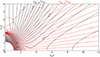 |
Fig. 6. Similar to Fig. 3, but for the first transverse overtone. |
| In the text | |
|
Fig. 7. Similar to Fig. 4, but for the first transverse overtone. Only a limited range is plotted for the quantity Λi because Λi takes up too diverse a range. Panel c overviews how the overtone behaves on the ky − kz plane. Trapped 3D modes are forbidden where |
| In the text | |
|
Fig. 8. Categorization of the y/t − z/t plane in terms of large-time expectations for the morphological features of impulsive kink motions. The bordering straight lines are determined by the limiting behavior of the group velocities as derived from Figs. 3 and 6. Line I+ pertains to B0-same-side fundamental modes, while line I− (II−) pertains to B0-straddling modes associated with the transverse fundamental (first overtone). Four sectors result. Different morphological features are expected for different sectors, the difference being particularly pronounced when line I− is crossed. One representative point in each sector (marked P1 to P4) is selected for further quantitative analysis (see text for more details). |
| In the text | |
Current usage metrics show cumulative count of Article Views (full-text article views including HTML views, PDF and ePub downloads, according to the available data) and Abstracts Views on Vision4Press platform.
Data correspond to usage on the plateform after 2015. The current usage metrics is available 48-96 hours after online publication and is updated daily on week days.
Initial download of the metrics may take a while.