| Issue |
A&A
Volume 707, March 2026
|
|
|---|---|---|
| Article Number | A15 | |
| Number of page(s) | 11 | |
| Section | Extragalactic astronomy | |
| DOI | https://doi.org/10.1051/0004-6361/202557483 | |
| Published online | 25 February 2026 | |
Temporal variability of polarization in blazars
1
DiSAT, Université dell’Insubria Via Valleggio 11 I-22100 Como, Italy
2
INAF – Osservatorio Astronomico di Brera Via E. Bianchi 46 I-23807 Merate, Italy
3
Gran Sasso Science Institute Viale F. Crispi 7 I-67100 L’Aquila, Italy
★ Corresponding author: This email address is being protected from spambots. You need JavaScript enabled to view it.
Received:
30
September
2025
Accepted:
10
January
2026
Abstract
We investigated the temporal variability of the polarization of synchrotron radiation from blazar jets. Multiwavelength observations reveal high-amplitude rotations of the electric vector position angle (EVPA), both in the optical and in the X-rays. The polarization degree and the EVPA often show seemingly erratic variability. To interpret these observations, we present a geometric and deterministic model in which off-axis, compact emitting features (i.e., blobs) propagate along the jet at the local flow velocity. The jet’s electromagnetic fields determine the dynamics of the blobs, which we calculated self-consistently using an analytical model of magnetically dominated outflows. The jet is axisymmetric, and its electromagnetic fields lack a turbulent component. We show that the observed polarization is sensitive to the blobs’ initial spatial configurations. For the same jet structure, we observe several remarkably complex polarization patterns, including large EVPA rotations of 180° or more in both directions and more erratic fluctuations. Simultaneous high-amplitude variations of the polarization degree and the EVPA can coincide with peaks in the observed luminosity. However, seemingly uncorrelated variations are also possible. We discuss the feasibility of constraining the particle acceleration mechanism from multifrequency polarimetric observations.
Key words: polarization / radiation mechanisms: non-thermal / galaxies: jets
© The Authors 2026
 Open Access article, published by EDP Sciences, under the terms of the Creative Commons Attribution License (https://creativecommons.org/licenses/by/4.0), which permits unrestricted use, distribution, and reproduction in any medium, provided the original work is properly cited.
This article is published in open access under the Subscribe to Open model. This email address is being protected from spambots. You need JavaScript enabled to view it. to support open access publication.
1. Introduction
Relativistic jets from supermassive black holes (SMBHs) in active galactic nuclei (AGNs) are highly collimated outflows of magnetized plasma. Charged particles produce non-thermal radiation spanning the entire electromagnetic spectrum, from the radio band to very high-energy gamma rays (Blandford et al. 2019). Blazars, a subclass of AGNs in which the jet is closely aligned to our line of sight, are optimal probes of jet physics, as the non-thermal radiation is strongly beamed due to this favorable orientation (Romero et al. 2017; Böttcher 2019).
The broadband spectral energy distribution (SED) of blazars exhibits a double-humped shape that peaks in the IR-soft-X-ray band and in the MeV-TeV band (e.g., Fossati et al. 1998). The low-energy portion of the SED is attributed to synchrotron radiation emitted by non-thermal electrons. Depending on the peak frequency of the synchrotron component, νpeak, blazars can be classified as high-synchrotron-peaked (HSP), intermediate-synchrotron-peaked (ISP), and low-synchrotron-peaked (LSP) types (e.g., Ajello et al. 2022). The HSP blazars have νpeak > 1015 Hz, the ISP blazars have 1014 Hz < νpeak < 1015 Hz, and the LSP blazars have νpeak < 1014 Hz. Most HSP and ISP blazars are classified as BL Lacertae (BL Lac) objects, whereas LSP blazars include both flat-spectrum radio quasars (FSRQs) and BL Lacs.
Because synchrotron radiation, which produces the low-energy part of the SED, is intrinsically linearly polarized, polarimetry has attracted significant attention as a key diagnostic of blazar jets. Observations of blazars in the quiescent state show that the optical polarization degree, ΠO, ranges from a few percent to 30%. In HSP blazars, where both optical and X-ray emission arise from synchrotron radiation, the X-ray polarization degree is significantly higher than the optical degree: ΠX/ΠO ≳ 2 (e.g., Liodakis et al. 2022; Di Gesu et al. 2022; Kouch et al. 2024).
Episodes of optical polarization variability in blazars were reported during the Robopol monitoring campaigns (Pavlidou et al. 2014). These observations revealed that both the polarization degree and the electric vector position angle (EVPA) exhibit significant variations, especially during active states (e.g., Marscher et al. 2008, 2010; Blinov et al. 2016, 2018). A notable feature is that the EVPA can undergo substantial rotations, or “swings” (Marscher et al. 2008, 2010; Abdo et al. 2010b; Larionov et al. 2013; Blinov et al. 2015, 2016, 2018; Kiehlmann et al. 2016). Rotations of the EVPA with amplitudes ≳90° are relatively rare events, although larger swings have been reported (Marscher et al. 2008, 2010; Chandra et al. 2015). The largest EVPA rotation detected to date reached ∼720° in PKS 1510-089 (Marscher et al. 2010). The timescales of EVPA rotations range from weeks to a few hours (Marscher et al. 2010; Blinov et al. 2015). Interestingly, the EVPA can rotate in both directions within the same source (Chandra et al. 2015).
Swings in the EVPA are often accompanied by γ-ray flares and a temporary decrease in the optical polarization degree (Blinov et al. 2015, 2016, 2018; Kiehlmann et al. 2016). The connection between wide rotations and multiwavelength flares (Abdo et al. 2010a; Marscher et al. 2010; Aleksić et al. 2014) is interpreted as evidence that EVPA swings result from a deterministic mechanism (Blinov et al. 2018). However, the overall temporal polarization pattern often appears erratic, which may indicate a stochastic process (Marscher 2014; Kiehlmann et al. 2017).
The recent launch of the Imaging X-ray Polarimetry Explorer satellite (IXPE; Weisskopf et al. 2022) has extended polarimetric observations to the X-ray domain, making it possible to perform multiwavelength polarimetric campaigns (Liodakis et al. 2022; Di Gesu et al. 2022, 2023; Ehlert et al. 2023; Middei et al. 2023a,b; Peirson et al. 2023; Chen et al. 2024; Errando et al. 2024; Kim et al. 2024; Kouch et al. 2024; Marshall et al. 2024; Abe et al. 2025; Agudo et al. 2025; Liodakis et al. 2025; Lisalda et al. 2025; Pacciani et al. 2025). Several IXPE observations target HSP blazars, in which X-rays are produced through synchrotron radiation. In principle, polarimetric observations of HSP blazars can reveal the magnetic field structure within the acceleration site (Tavecchio 2021). The IXPE mission detected EVPA swings in the X-ray band that are not associated with simultaneous optical swings (Di Gesu et al. 2023; Kim et al. 2024). These observations are interpreted as evidence that electrons are accelerated by a shock moving along a helical trajectory (Di Gesu et al. 2023). Swings of the EVPA in the X-ray band arise because the emitting electrons illuminate a small region of the jet downstream of the shock. By contrast, the optical EVPA does not rotate because the emitting electrons are distributed more uniformly as a result of their longer cooling times. However, the energy-stratified shock model can hardly explain the optical EVPA swings without a simultaneous swing in the X-ray band (Middei et al. 2023b). We emphasize that energy stratification of the emitting electrons is not a unique signature of the shock acceleration scenario, but is a generic by-product of any spatially localized acceleration process (Bolis et al. 2024a; Zhang et al. 2024).
The discovery of polarization variability has led to several theoretical studies aimed at interpreting this behavior (for a review, see Zhang 2019). Swings of the EVPA have been attributed to geometric effects (e.g., Marscher et al. 2008, 2010; Nalewajko 2010; Larionov et al. 2013; Lyutikov & Kravchenko 2017; Peirson & Romani 2018) or physical effects, including changes in magnetic field structure due to shocks (Konigl & Choudhuri 1985; Zhang et al. 2014, 2015, 2016), and to current-driven kink instabilities (Nalewajko 2017; Zhang et al. 2017). Random-walk processes have been invoked to interpret the erratic variability of polarization (Kiehlmann et al. 2017). Scenarios in which both deterministic and stochastic mechanisms coexist in the same source (e.g., shock waves in turbulent magnetic fields) have also been considered (Marscher 2014; Angelakis et al. 2016; Tavecchio et al. 2018). Recent fully kinetic particle-in-cell (PIC) simulations show that EVPA swings may result from magnetic reconnection events (Zhang et al. 2018; Hosking & Sironi 2020). In the reconnection scenario, the EVPA swings are associated with high-energy outbursts.
In this work, we propose a geometric and deterministic model to interpret polarization variability. Following the approach of Marscher et al. (2008, 2010) and Larionov et al. (2013), we considered compact, off-axis emitting features (i.e., blobs) propagating along the jet at the local flow velocity (see Fig. 1). The key aspect of our model is that, unlike previous approaches, the blob’s trajectory is computed self-consistently. Its dynamics is dictated by the structure of jet electromagnetic fields, whose profile is derived from a model of magnetically driven outflows (Lyubarsky 2009). We did not assume any specific acceleration mechanism for the emitting particles. Polarization variability is determined solely by kinematics effects (i.e., relativistic beaming and light-travel time delays). We find that even a geometric and deterministic model can produce remarkably complex polarization patterns, including large EVPA rotations and seemingly erratic variability.
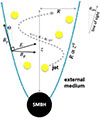 |
Fig. 1. Schematic of the jet model. The equilibrium boundary radius of the jet, R, is proportional to zq, where z is the distance from the supermassive black hole. The parameter q < 1 depends on the pressure profile of the external medium that collimates the jet. We consider a cylindrical jet (q = 0), a “sausage-like” jet (q = 0.3), and a nearly parabolic jet (q = 0.4). In the sausage-like jet, the boundary oscillates about the equilibrium value. The emission originates from an ensemble of compact, off-axis emission features (yellow blobs) that propagate along the jet at the local flow velocity. The line of sight forms an angle θobs with the jet axis. |
The paper is organized as follows. In Sect. 2, we describe the jet model adopted in this work. In Sect. 3, we present our results. In Sect. 4, we discuss their implications and summarize our conclusions.
2. Physical model
According to the leading theoretical model, relativistic jets are powered by the extraction of magnetic energy from rotating SMBHs (e.g., Blandford & Znajek 1977; Vlahakis & Königl 2004; Tchekhovskoy et al. 2011). Jet power remains dominated by Poynting flux in the region where optical and X-ray emissions are produced (Lyubarsky 2010). The structure of magnetically dominated jets has been extensively studied using both analytical methods (Beskin et al. 1998, 2004; Vlahakis 2004; Lyubarsky 2009, 2010) and numerical simulations (Komissarov et al. 2007, 2009; Tchekhovskoy et al. 2009, 2011).
2.1. Jet structure
Our jet model is based on the work of Lyubarsky (2009), who derived asymptotic equations (valid far from the light cylinder) to describe axisymmetric, stationary, Poynting-dominated magnetohydrodynamic (MHD) outflows. The external pressure that confines the outflow decreases as a power law, 𝒫ext ∝ z−κ, where z denotes the distance from the SMBH. When κ ≤ 2, the jet has a parabolic shape, R ∝ zq, where R is the transverse radius of the jet and the parameter q < 1 depends on the power-law index κ of the external pressure profile. For 0 < κ < 2, q = κ/4, while for a wind-like medium with κ = 2, 1/2 < q < 1. Throughout this work, we focused on solutions with κ < 2, so that q < 1/2. We adopted cylindrical coordinates (R, ϕ, z), with the z axis aligned along the jet direction. Quantities without a prime are defined in the observer frame, whereas primed quantities are defined in the jet frame. For simplicity, we assumed that the SMBH is located at redshift z = 0.
The electromagnetic fields in the observer frame are expressed as
 (1)
(1)
 (2)
(2)
The components of the electromagnetic fields are given by
 (3)
(3)
 (4)
(4)
where Θ denotes the local opening angle of the jet. We adopted units in which the speed of light is set to c = 1. We assumed the angular velocity Ω and the poloidal magnetic field Bp to be independent of R. Numerical simulations support this approximation (see e.g., Fig. 4 of Komissarov et al. 2007).
The shape of the magnetic flux surfaces, where the flux function ψ is constant, is given by Eq. (74) of Lyubarsky (2009):
 (5)
(5)
The dimensionless function Y(Ωz) is defined by Eqs. (81)–(82) of Lyubarsky (2009) as
![Mathematical equation: $$ \begin{aligned} Y= K \,\left(\Omega z\right)^q \Bigg [ \frac{1}{C_1} \cos ^2 S + C_1 \Big ( C_2\cos S + \frac{\pi }{2-4q} \sin S \Big )^2\Bigg ]^{1/2}\, , \end{aligned} $$](/articles/aa/full_html/2026/03/aa57483-25/aa57483-25-eq6.gif) (6)
(6)
where
 (7)
(7)
In the above equations, β ∼ 1 denotes the ratio of the external pressure to the magnetic pressure at the light cylinder, while C1 and C2 are free parameters.
The local opening angle of the jet, Θ, can be expressed as (Lyubarsky 2009; Bolis et al. 2024a)
 (8)
(8)
and the toroidal magnetic field is given by
 (9)
(9)
The poloidal magnetic field is given by Eq. (5) of Lyubarsky (2009), which is  . Its magnitude is
![Mathematical equation: $$ \begin{aligned} B_{\rm p} = \frac{2\,\psi _0}{\sqrt{3}\,Y^2}\, \sqrt{1+\sqrt{3} \left(\frac{\psi }{ \psi _0}\right)\left[ \frac{\mathrm{d} Y}{\mathrm{d} \left(\Omega z\right)}\right]^2}\;. \end{aligned} $$](/articles/aa/full_html/2026/03/aa57483-25/aa57483-25-eq11.gif) (10)
(10)
Since the outflow is magnetically dominated, we assumed that the bulk velocity of the fluid, v, coincides with the drift velocity: v = E × B/B2. The corresponding bulk Lorentz factor is Γ = (1 − v2)−1/2 = (1 − E2/B2)−1/2.
2.2. Time-dependent polarimetry of moving blobs
In the fluid proper frame, the distribution of emitting electrons is isotropic in momentum and follows a power law in energy:
 (11)
(11)
where Ke(t, R, ϕ, z) is the proper number density, γe is the Lorentz factor of the electrons, and p is the electron power-law index.
We calculated the time-dependent polarization of synchrotron radiation as follows. We included emission from an ensemble of bright off-axis compact features (blobs) that propagate with the local bulk velocity of the fluid. We assumed that all the blobs were identical. The calculation of the Stokes parameters (I, Q, U) of a single blob is described in detail in Appendix A. Because we considered ultra-relativistic particles, we neglected circular polarization and set V = 0 (where V is the fourth Stokes parameter). The normalized Stokes parameters of the ensemble of blobs are defined as
 (12)
(12)
 (13)
(13)
 (14)
(14)
where the index i refers to the i-th blob, and Nblobs is the total number of blobs. We considered a single-blob scenario (Nblobs = 1) and another with multiple blobs (Nblobs = 10). Multiple blobs may occur if the particles are accelerated at different reconnection sites. We verified that our results remain qualitatively similar if Nblobs increases or decreases by a factor of a few relative to the fiducial value (Nblobs = 10). The normalization of the Stokes parameters is irrelevant for calculating the polarization degree and the EVPA, which depend on the ratios Qblobs/Iblobs and Ublobs/Iblobs. With the normalization of Eqs. (12)–(14), the total radiation intensity is independent of Nblobs. Varying Nblobs is equivalent to modifying the spatial distribution of the emitting particles, while keeping their total number constant.
We considered that part of the synchrotron radiation was produced by a nearly axisymmetric jet. We modeled the jet as an additional ensemble of Njet blobs that propagate with the local bulk velocity of the fluid. The normalized Stokes parameters of the jet are defined as
 (15)
(15)
 (16)
(16)
 (17)
(17)
We assumed that Njet is very large (i.e., Njet ≫ Nblobs). The normalized Stokes parameters of the jet are then independent of the exact value of Njet because the distribution of the blobs is nearly axisymmetric (we find that Njet = 105 is sufficient for our scope).
We obtained the final values of the Stokes parameters by summing the contributions from the blobs and the jet:
 (18)
(18)
 (19)
(19)
 (20)
(20)
where ηjet is a weighting factor. We considered two scenarios: one in which the axisymmetric jet was absent (ηjet = 0), and one in which the jet and blobs had similar luminosities1 (ηjet = 1). The polarization degree, Π, and the EVPA, Ψ, are given by
 (21)
(21)
2.3. Model parameters
We assumed a viewing angle of θobs = 0.1 rad and an angular velocity of Ω = 10−5 s−1. This choice yields Γ ∼ 10 at the distance from the SMBH where the non-thermal emission is produced (z ∼ 1017 − 1018 cm). We assumed that the blobs were located near the boundary radius of the jet (i.e., on the surface that separates the jet from the external medium). We therefore set ψ = ψ0 in Eqs. (5)–(9). Our choice is appropriate if the particles are accelerated by shear flow near the boundary radius (e.g., Sironi et al. 2021).
In the single-blob scenario (Nblobs = 1), we list the coordinates of the blob at the initial time t = 0 (namely, ϕ0, z0, R0) in Table 1. The coordinate R0 is determined by the condition that the blob is located near the boundary radius of the jet. In the multi-blob scenario (Nblobs = 10), we spaced the blobs over the jet at the initial time t = 0. We assigned the initial coordinates of the first blob as in the single-blob scenario. We drew the initial coordinates of the other blobs from a uniform distribution in the range 0 < ϕ < 2π, z0 < z < 1.5 z0 (where z0 is the initial distance of the first blob from the SMBH). In the axisymmetric jet (which is modeled as an ensemble of Njet = 105 blobs), we drew the initial coordinates of the blobs from the same uniform distribution in the range 0 < ϕ < 2π, z0 < z < 1.5 z0. We used a sufficiently large simulation volume to ensure that the blobs remained within it over the timescale of our simulation as they moved along the jet.
Initial and final parameter values for the single-blob scenario.
We adopted a power-law index of p = 4 for the electrons. The corresponding spectrum of synchrotron radiation is Fν ∝ ν−α, where α = (p − 1)/2 = 1.5 is the photon index. The X-ray spectral index of HSP blazars typically lies in the range α ∼ 1 − 2, which is similar to the optical spectral index of LSP and ISP blazars (e.g., Fossati et al. 1998; Abdo et al. 2011; Ghisellini et al. 2017). The magnitude of the polarization degree can vary by a factor of a few for different values of p. However, the temporal pattern remains qualitatively similar.
3. Results
Very long baseline interferometry imaging of radio emission from AGN jets suggests that the jet shape is nearly parabolic (Mertens et al. 2016; Pushkarev et al. 2017; Kovalev et al. 2020; Boccardi et al. 2021). Imaging of the jet in M87 suggests a “sausage-like” shape, in which the jet radius oscillates about the parabolic profile (see Fig. 6 of Mertens et al. 2016). However, most observations constrain the jet shape on scales of tens of parsecs, which is significantly larger than the distance from the SMBH where the blazar emission is produced. We considered three different jet structures:
-
Cylindrical jet. We set q = 0, C1 = 2/π, and C2 = 0 in Eq. (6). The transverse radius of the jet is constant.
-
Sausage-like jet. We set q = 0.3 and C1 = (2−4q)/π in Eq. (6). We considered two cases: C2 = 0.8 and C2 = 2. The transverse radius of the jet oscillates about the equilibrium position, which is R ∝ zq. The amplitude of the oscillations increases for large C2 (there would be no oscillations for C2 = 0).
-
Nearly parabolic jet. We set q = 0.4, C1 = (2−4q)/π, and C2 = 0 in Eq. (6). The transverse radius is R ∝ zq.
Figure 2 shows the jet transverse radius and the bulk Lorentz factor as functions of the distance from the black hole for different jet structures. For each jet structure, we calculated the time-dependent Stokes parameters for the emission scenarios described in Sect. 2.2. Table B.1 summarizes our results.
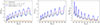 |
Fig. 2. Jet transverse radius normalized to its minimum value, R/Rmin (left panel); bulk Lorentz factor in the proper frame normalized to its minimum value, Γ/Γmin (middle panel); and poloidal magnetic field magnitude normalized to its minimum value, Bp/Bp, min (right panel), shown as functions of distance from the black hole expressed in units of c/Ω, for different jet shapes. |
For the cylindrical jet structure (q = 0), the temporal profiles of the single blob Stokes parameters are periodic. Different initial blob conditions produce a phase shift in the observed emission. For the other jet structures (q ≠ 0), the temporal profiles are not strictly periodic. The initial conditions of the blob influence the observed emission. To illustrate this effect, for q = 0.4, we investigated two models (single blob A and single blob B) that differ only in the initial phase of the blob. In the multiple-blob scenario, we randomly chose the initial phases of the blobs. Since the number of blobs is relatively large (Nblobs = 10), the temporal profiles of the Stokes parameters are qualitatively similar. For example, the amplitude of the EVPA rotations varies by < 50% for different realizations.
3.1. Cylindrical jet
Figure 3 shows the time evolution of the polarization degree, Π, the EVPA, Ψ, and the intensity normalized to its maximum value, I/Imax, for a cylindrical jet. The top panels correspond to the single-blob scenario (Nblobs = 1). The nearly axisymmetric jet may or may not contribute to the observed emission.
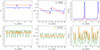 |
Fig. 3. Polarization degree, Π (left panels); electric vector position angle (EVPA), Ψ (middle panels); and intensity normalized to its maximum value, I/Imax (right panels) plotted as a function of time in the observed frame, tobs, measured in days. The jet has a cylindrical shape. Top panels: Emission from a single blob (Nblobs = 1 and ηjet = 0; dashed line) and from a single blob plus a nearly axisymmetric jet (Nblobs = 1 and ηjet = 1; solid line). Bottom panels: Emission from multiple blobs (Nblobs = 10 and ηjet = 0; dashed line) and from multiple blobs plus a nearly axisymmetric jet (Nblobs = 10 and ηjet = 1; solid line). |
When ηjet = 0, the polarization degree is equal to Π0 = (p + 1)/(p + 7/3), as expected for a uniform electromagnetic field. For Nblobs = 1 and ηjet = 0, Π = Π0, regardless of jet shape. The EVPA shows a rapid rotation, ΔΨ ∼ 60°, on a timescale Δtobs ∼ 1.5 days, which coincides with the peak of the observed intensity (when the blob velocity aligns with the line of sight). When ηjet = 1, the polarization degree is lower than Π0 for most of the time and approaches Π0 when the blob dominates the observed emission. In this case, the EVPA is constant (Ψ ≃ π/2) when the jet dominates the observed emission and varies when the blob dominates.
The bottom panels of Fig. 3 correspond to the multiple-blob scenario (Nblobs = 10). In this case, we observe a periodic behavior in Π, Ψ, and I/Imax with an observed period of approximately 11 days, which is the same as in the single-blob scenario. The amplitude of the variations is greater when ηjet = 0, with ΔΠ ∼ 0.40 and ΔΨ ∼ 55°. The variations are smaller when ηjet = 1, because the Stokes parameters of the jet (Ijet, Qjet , and Ujet) are nearly constant. For example, since we modeled the jet as an ensemble of a very large number of blobs (Njet = 105), intensity variations are erased: at any given time, many blobs are directed along the line of sight.
3.2. Sausage-like jet
Figures 4 and 5 show the time evolution of Π, Ψ, and I/Imax for a sausage-like jet. In Fig. 4 we adopt C2 = 0.8, whereas in Fig. 5 we adopt C2 = 2. The intensity peaks occur when the blob velocity is aligned with the line of sight. However, the blob trajectory is complex because the rotation period in the ϕ direction is not connected with the oscillations of the jet radius along the z direction. As a result, we do not observe periodic behavior in Π, Ψ, and I/Imax.
The case C2 = 0.8, shown in Fig. 4, corresponds to smaller oscillations of the jet transverse radius about the equilibrium position with respect to C2 = 2. In the single-blob scenario, when ηjet = 0, the EVPA exhibits smooth variations of amplitude ΔΨ ∼ 77°. When ηjet = 1, the polarization degree approaches Π0 as the blob dominates the observed emission. The EVPA remains nearly constant, except for a sudden jump of approximately ΔΨ ∼ 60° at tobs ∼ 14 days, which occurs when the intensity reaches I ∼ Imax.
In the multiple-blob scenario, when ηjet = 0, we observe significant variability in both Π and Ψ. The variability pattern is complex and seemingly erratic, despite arising from a deterministic geometric model. We observe a rapid EVPA jump of approximately ΔΨ ∼ 80° over a timescale of 1 − 2 days at tobs ∼ 12 days, associated with a sharp decrease in the polarization degree (ΔΠ ∼ 0.55). This jump occurs when I ∼ Imax. When ηjet = 1, we observe a similar behavior, although the amplitude of the jumps is smaller.
The case C2 = 2, shown in Fig. 5, corresponds to larger oscillations of the jet transverse radius about the equilibrium position with respect to C2 = 0.8. In the single-blob scenario, when ηjet = 0, we observe a large EVPA rotation (ΔΨ ∼ 720° ) over a period of six days. The rotation is associated with an increase in intensity from the minimum to 85% of its maximum value. When the intensity reaches its peak at tobs ∼ 4.5 days and subsequently decreases, the EVPA undergoes a smaller jump of ∼90°. When ηjet = 1, both the polarization degree and the intensity exhibit two peaks. The polarization degree varies by ΔΠ ∼ 0.60. The EVPA remains nearly constant, except for a sharp rotation of approximately ΔΨ ∼ 80° occurring between tobs ∼ 15 − 16 days, close to the intensity maximum.
In the multiple-blob scenario, as previously described for the cylindrical jet, we observe a complex evolution of all observables. When ηjet = 0, the polarization degree exhibits an abrupt jump at tobs ∼ 5 days, increasing from Π ∼ 0 to Π ∼ Π0 on a timescale of less than a day. During the same interval, the EVPA undergoes a rotation of approximately 100°. Over a timescale of one week, the EVPA rotates by ΔΨ ∼ 390°. When ηjet = 1, the variability of the observables is less extreme.
3.3. Nearly parabolic jet
Figure 6 shows the time evolution of Π, Ψ, and I/Imax for a nearly parabolic jet. We consider two scenarios with a single blob (single blob A and single blob B), which differ only in the initial blob coordinates listed in Table 1.
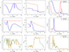 |
Fig. 6. Same as Fig. 3, but for a parabolic jet shape. The first row (single blob A) and the second row (single blob B) differ only in the initial blob coordinates. |
Large EVPA rotations (ΔΨ > 180°) may or may not occur depending on the initial coordinates of the blob, which affect its Doppler factor. For the single blob A, when ηjet = 0, we observe a rotation of ΔΨ ∼ 350°. The fastest rotation rate is associated with a double-peaked intensity structure, with peaks at tobs ∼ 11 days and tobs ∼ 13 days. For the single blob B case, when ηjet = 0, we observe a smaller rotation followed by a counter-rotation (ΔΨ ∼ 80°), which is associated with an intensity peak. When ηjet = 1, we observe ΔΠ ∼ 0.65 and ΔΨ ∼ 118° for the single blob A, while we observe ΔΠ ∼ 0.69 and ΔΨ ∼ 127° for the single blob B.
In the multiple-blob scenario, the polarization degree fluctuates substantially, giving the impression of erratic variability, whereas the EVPA rotates more smoothly. We observe large EVPA rotations, with ΔΨ ∼ 342° when ηjet = 0 and ΔΨ ∼ 334° when ηjet = 1. We emphasize that for ηjet = 0, large EVPA rotations (ΔΨ > 180°) occur in both directions, clockwise and counterclockwise.
4. Discussion
We investigated the temporal variability of the polarization of the synchrotron radiation from blazar jets using a geometric and deterministic model. Following Marscher et al. (2008), we considered off-axis emission features (blobs) that propagate along the jet with the local bulk velocity of the fluid. We computed the jet electromagnetic fields and the bulk velocity self-consistently using the jet model of Lyubarsky (2009). The jet is axisymmetric, and its electromagnetic fields do not contain a turbulent component. We did not assume a specific particle acceleration mechanism. Blobs may form if the acceleration sites are localized, for example, as a result of intermittency in a turbulent cascade (Comisso & Sironi 2018, 2019).
We explored several scenarios corresponding to different jet shapes and different initial blob configurations. We find that the temporal variability of the polarization does not follow a universal trend. Our model shows both smooth, continuous variations and seemingly erratic fluctuations of the polarization degree and the electric vector position angle (EVPA). As noted previously by Lyutikov & Kravchenko (2017), a geometric and deterministic model can produce such features. Interestingly, the same jet shape can produce a different temporal evolution of the polarization degree and EVPA by changing the initial spatial configuration of the blobs.
Our model produces remarkably complex polarization patterns. We observed the following features in the temporal evolution of the polarization degree and EVPA.
-
There is no clear correlation between the polarization degree and the EVPA. During EVPA rotations, the polarization degree can remain constant or suddenly jump from its minimum to its maximum value.
-
Simultaneous high-amplitude variations of the polarization degree and the EVPA can coincide with sharp peaks in the observed luminosity.
-
Bidirectional EVPA rotations (both clockwise and counterclockwise) are possible for the same jet shape. Large EVPA rotations of 180° or more are occasionally observed.
-
The polarization degree and the EVPA show significant variability over a broad range of timescales for the same jet shape, from a few hours to several days or even weeks.
These findings aid in the interpretation of the polarimetric variability signatures. The RoboPol monitoring program detected several large optical EVPA rotations that are frequently associated with multiwavelength flares (e.g., Marscher et al. 2008, 2010; Blinov et al. 2016, 2018). However, in many cases, the polarization degree and the EVPA patterns are not correlated with flux variability, and their evolution appears to be erratic (Marscher 2014; Kiehlmann et al. 2017).
More recently, the launch of the IXPE satellite has enabled multiwavelength polarimetric studies of HSP blazars. Interestingly, simultaneous X-ray and optical EVPA observations show that their variability is often uncorrelated. During a five-day monitoring campaign of Mkn 421, Di Gesu et al. (2023) reported a ∼360° EVPA rotation in the X-ray band, with no corresponding rotation observed at lower frequencies. The polarization degree remained relatively stable throughout the event and showed a strong chromaticity.
Middei et al. (2023b) reported the first orphan optical EVPA rotation. In PG 1553+113, the optical EVPA changed by approximately 125°, with no simultaneous rotation observed in the X-ray band. The polarization degree showed no substantial variability during the event. Kouch et al. (2024) reported another orphan optical EVPA rotation in PKS 2155-304. The optical EVPA rotated approximately 50° in one direction and then 40° in the opposite direction, while the X-ray EVPA remained stable. This behavior demonstrates that clockwise and counterclockwise EVPA rotations can occur within the same source.
During the first IXPE pointing of Mkn 421 in May 2022, Kim et al. (2024) detected an X-ray EVPA rotation of approximately 180°, while the X-ray polarization degree remained nearly constant. A subsequent EVPA rotation in June 2022 was accompanied by simultaneous spectral variations. Interestingly, at longer wavelengths, the EVPA rotated in the opposite direction with respect to the X-ray EVPA, and the rotation occurred over a longer timescale.
During an optical–X-ray flaring episode of the LSP blazar S4 0954+65, Kouch et al. (2025) observed two orphan optical EVPA rotations: one of approximately 85° that lasted one day and another of ∼87° that lasted two days. In contrast, during the same flaring episode, the X-ray polarization degree varied by a factor of two, whereas the optical polarization degree remained stable.
According to the standard interpretation of the IXPE collaboration (Di Gesu et al. 2023), temporal variability of polarization indicates that non-thermal particles are accelerated by shocks moving along a helical trajectory. This interpretation explains orphan X-ray EVPA rotations because the accelerated particles are energy stratified. The optical EVPA does not rotate because the emitting electrons are distributed more uniformly because of their longer cooling time. However, this model cannot explain orphan optical EVPA rotations.
We note that in our model the time evolution of the polarization degree and EVPA is generic (i.e., it does not specifically apply to a particular band and can be used for both optical and X-ray observations). It is plausible that the spectral properties of the blobs and the background differ for different bands. This would add more complexity to the scenario. The observation of non-simultaneous optical and X-ray EVPA rotations indicates that the ratio of the background emission (produced by a nearly axisymmetric jet) to the emission from the blobs can be strongly chromatic. Large EVPA rotations can be produced when the blobs dominate the observed emission, whereas more erratic variability is expected when the jet emission is stronger. It remains unclear whether the particle acceleration mechanism can be constrained based on these relatively straightforward considerations. As discussed previously by Bolis et al. (2024a,b), constraining the acceleration mechanism from multifrequency polarimetric observations remains extremely challenging.
Acknowledgments
We thank the anonymous referee for their constructive comments that improved the paper. We acknowledge financial support from a Rita Levi Montalcini fellowship (PI E. Sobacchi) and an INAF Theory Grant 2024 (PI F. Tavecchio). This work has been funded by the European Union-Next Generation EU, PRIN 2022 RFF M4C21.1 (2022C9TNNX).
References
- Abdo, A. A., Ackermann, M., Agudo, I., et al. 2010a, ApJ, 716, 30 [NASA ADS] [CrossRef] [Google Scholar]
- Abdo, A. A., Ackermann, M., Ajello, M., et al. 2010b, Nature, 463, 919 [NASA ADS] [CrossRef] [Google Scholar]
- Abdo, A. A., Ackermann, M., Ajello, M., et al. 2011, ApJ, 736, 131 [Google Scholar]
- Abe, K., Abe, S., Abhir, J., et al. 2025, A&A, 694, A195 [NASA ADS] [CrossRef] [EDP Sciences] [Google Scholar]
- Agudo, I., Liodakis, I., Otero-Santos, J., et al. 2025, ApJ, 985, L15 [Google Scholar]
- Ajello, M., Baldini, L., Ballet, J., et al. 2022, ApJS, 263, 24 [NASA ADS] [CrossRef] [Google Scholar]
- Aleksić, J., Ansoldi, S., Antonelli, L. A., et al. 2014, A&A, 567, A41 [NASA ADS] [CrossRef] [EDP Sciences] [Google Scholar]
- Angelakis, E., Hovatta, T., Blinov, D., et al. 2016, MNRAS, 463, 3365 [NASA ADS] [CrossRef] [Google Scholar]
- Beskin, V. S., Kuznetsova, I. V., & Rafikov, R. R. 1998, MNRAS, 299, 341 [CrossRef] [Google Scholar]
- Beskin, V. S., Zakamska, N. L., & Sol, H. 2004, MNRAS, 347, 587 [Google Scholar]
- Blandford, R., Meier, D., & Readhead, A. 2019, ARA&A, 57, 467 [NASA ADS] [CrossRef] [Google Scholar]
- Blandford, R. D., & Znajek, R. L. 1977, MNRAS, 179, 433 [NASA ADS] [CrossRef] [Google Scholar]
- Blinov, D., Pavlidou, V., Papadakis, I., et al. 2015, MNRAS, 453, 1669 [NASA ADS] [CrossRef] [Google Scholar]
- Blinov, D., Pavlidou, V., Papadakis, I. E., et al. 2016, MNRAS, 457, 2252 [NASA ADS] [CrossRef] [Google Scholar]
- Blinov, D., Pavlidou, V., Papadakis, I., et al. 2018, MNRAS, 474, 1296 [CrossRef] [Google Scholar]
- Boccardi, B., Perucho, M., Casadio, C., et al. 2021, A&A, 647, A67 [NASA ADS] [CrossRef] [EDP Sciences] [Google Scholar]
- Bolis, F., Sobacchi, E., & Tavecchio, F. 2024a, A&A, 690, A14 [NASA ADS] [CrossRef] [EDP Sciences] [Google Scholar]
- Bolis, F., Sobacchi, E., & Tavecchio, F. 2024b, Phys. Rev. D, 110, 123032 [Google Scholar]
- Böttcher, M. 2019, Galaxies, 7, 20 [Google Scholar]
- Chandra, S., Zhang, H., Kushwaha, P., et al. 2015, ApJ, 809, 130 [CrossRef] [Google Scholar]
- Chen, C.-T. J., Liodakis, I., Middei, R., et al. 2024, ApJ, 974, 50 [NASA ADS] [CrossRef] [Google Scholar]
- Comisso, L., & Sironi, L. 2018, Phys. Rev. Lett., 121, 255101 [NASA ADS] [CrossRef] [Google Scholar]
- Comisso, L., & Sironi, L. 2019, ApJ, 886, 122 [Google Scholar]
- Del Zanna, L., Volpi, D., Amato, E., & Bucciantini, N. 2006, A&A, 453, 621 [NASA ADS] [CrossRef] [EDP Sciences] [Google Scholar]
- Di Gesu, L., Donnarumma, I., Tavecchio, F., et al. 2022, ApJ, 938, L7 [CrossRef] [Google Scholar]
- Di Gesu, L., Marshall, H. L., Ehlert, S. R., et al. 2023, Nat. Astron., 7, 1245 [NASA ADS] [CrossRef] [Google Scholar]
- Ehlert, S. R., Liodakis, I., Middei, R., et al. 2023, ApJ, 959, 61 [NASA ADS] [CrossRef] [Google Scholar]
- Errando, M., Liodakis, I., Marscher, A. P., et al. 2024, ApJ, 963, 5 [NASA ADS] [CrossRef] [Google Scholar]
- Fossati, G., Maraschi, L., Celotti, A., Comastri, A., & Ghisellini, G. 1998, MNRAS, 299, 433 [Google Scholar]
- Ghisellini, G., Righi, C., Costamante, L., & Tavecchio, F. 2017, MNRAS, 469, 255 [NASA ADS] [CrossRef] [Google Scholar]
- Hosking, D. N., & Sironi, L. 2020, ApJ, 900, L23 [NASA ADS] [CrossRef] [Google Scholar]
- Kiehlmann, S., Blinov, D., Pearson, T. J., & Liodakis, I. 2017, MNRAS, 472, 3589 [Google Scholar]
- Kiehlmann, S., Savolainen, T., Jorstad, S. G., et al. 2016, A&A, 590, A10 [NASA ADS] [CrossRef] [EDP Sciences] [Google Scholar]
- Kim, D. E., Di Gesu, L., Liodakis, I., et al. 2024, A&A, 681, A12 [NASA ADS] [CrossRef] [EDP Sciences] [Google Scholar]
- Komissarov, S. S., Barkov, M. V., Vlahakis, N., & Königl, A. 2007, MNRAS, 380, 51 [Google Scholar]
- Komissarov, S. S., Vlahakis, N., Königl, A., & Barkov, M. V. 2009, MNRAS, 394, 1182 [NASA ADS] [CrossRef] [Google Scholar]
- Konigl, A., & Choudhuri, A. R. 1985, ApJ, 289, 188 [Google Scholar]
- Kouch, P. M., Liodakis, I., Middei, R., et al. 2024, A&A, 689, A119 [NASA ADS] [CrossRef] [EDP Sciences] [Google Scholar]
- Kouch, P. M., Liodakis, I., Fenu, F., et al. 2025, A&A, 695, A99 [NASA ADS] [CrossRef] [EDP Sciences] [Google Scholar]
- Kovalev, Y. Y., Pushkarev, A. B., Nokhrina, E. E., et al. 2020, MNRAS, 495, 3576 [NASA ADS] [CrossRef] [Google Scholar]
- Larionov, V. M., Jorstad, S. G., Marscher, A. P., et al. 2013, ApJ, 768, 40 [NASA ADS] [CrossRef] [Google Scholar]
- Liodakis, I., Marscher, A. P., Agudo, I., et al. 2022, Nature, 611, 677 [CrossRef] [Google Scholar]
- Liodakis, I., Zhang, H., Boula, S., et al. 2025, A&A, 698, L19 [NASA ADS] [CrossRef] [EDP Sciences] [Google Scholar]
- Lisalda, L., Gau, E., Krawczynski, H., et al. 2025, ArXiv e-prints [arXiv:2507.07232] [Google Scholar]
- Lyubarsky, Y. 2009, ApJ, 698, 1570 [NASA ADS] [CrossRef] [Google Scholar]
- Lyubarsky, Y. 2010, MNRAS, 402, 353 [NASA ADS] [CrossRef] [Google Scholar]
- Lyutikov, M., & Kravchenko, E. V. 2017, MNRAS, 467, 3876 [Google Scholar]
- Lyutikov, M., Pariev, V. I., & Blandford, R. D. 2003, ApJ, 597, 998 [Google Scholar]
- Marscher, A. P. 2014, ApJ, 780, 87 [Google Scholar]
- Marscher, A. P., Jorstad, S. G., D’Arcangelo, F. D., et al. 2008, Nature, 452, 966 [Google Scholar]
- Marscher, A. P., Jorstad, S. G., Larionov, V. M., et al. 2010, ApJ, 710, L126 [Google Scholar]
- Marshall, H. L., Liodakis, I., Marscher, A. P., et al. 2024, ApJ, 972, 74 [NASA ADS] [CrossRef] [Google Scholar]
- Mertens, F., Lobanov, A. P., Walker, R. C., & Hardee, P. E. 2016, A&A, 595, A54 [NASA ADS] [CrossRef] [EDP Sciences] [Google Scholar]
- Middei, R., Liodakis, I., Perri, M., et al. 2023a, ApJ, 942, L10 [NASA ADS] [CrossRef] [Google Scholar]
- Middei, R., Perri, M., Puccetti, S., et al. 2023b, ApJ, 953, L28 [NASA ADS] [CrossRef] [Google Scholar]
- Nalewajko, K. 2010, Int. J. Mod. Phys. D, 19, 701 [Google Scholar]
- Nalewajko, K. 2017, Galaxies, 5, 64 [Google Scholar]
- Pacciani, L., Kim, D. E., Middei, R., et al. 2025, ApJ, 983, 78 [Google Scholar]
- Pavlidou, V., Angelakis, E., Myserlis, I., et al. 2014, MNRAS, 442, 1693 [NASA ADS] [CrossRef] [Google Scholar]
- Peirson, A. L., Negro, M., Liodakis, I., et al. 2023, ApJ, 948, L25 [NASA ADS] [CrossRef] [Google Scholar]
- Peirson, A. L., & Romani, R. W. 2018, ApJ, 864, 140 [NASA ADS] [CrossRef] [Google Scholar]
- Pushkarev, A. B., Kovalev, Y. Y., Lister, M. L., & Savolainen, T. 2017, MNRAS, 468, 4992 [Google Scholar]
- Romero, G. E., Boettcher, M., Markoff, S., & Tavecchio, F. 2017, Space Sci. Rev., 207, 5 [NASA ADS] [CrossRef] [Google Scholar]
- Sironi, L., Rowan, M. E., & Narayan, R. 2021, ApJ, 907, L44 [CrossRef] [Google Scholar]
- Tavecchio, F. 2021, Galaxies, 9, 37 [NASA ADS] [CrossRef] [Google Scholar]
- Tavecchio, F., Landoni, M., Sironi, L., & Coppi, P. 2018, MNRAS, 480, 2872 [NASA ADS] [CrossRef] [Google Scholar]
- Tchekhovskoy, A., McKinney, J. C., & Narayan, R. 2009, ApJ, 699, 1789 [NASA ADS] [CrossRef] [Google Scholar]
- Tchekhovskoy, A., Narayan, R., & McKinney, J. C. 2011, MNRAS, 418, L79 [NASA ADS] [CrossRef] [Google Scholar]
- Vlahakis, N. 2004, ApJ, 600, 324 [NASA ADS] [CrossRef] [Google Scholar]
- Vlahakis, N., & Königl, A. 2004, ApJ, 605, 656 [Google Scholar]
- Weisskopf, M. C., Soffitta, P., Baldini, L., et al. 2022, J. Astron. Telesc. Instrum. Syst., 8, 026002 [NASA ADS] [CrossRef] [Google Scholar]
- Zhang, H. 2019, Galaxies, 7, 85 [NASA ADS] [CrossRef] [Google Scholar]
- Zhang, H., Chen, X., & Böttcher, M. 2014, ApJ, 789, 66 [NASA ADS] [CrossRef] [Google Scholar]
- Zhang, H., Chen, X., Böttcher, M., Guo, F., & Li, H. 2015, ApJ, 804, 58 [NASA ADS] [CrossRef] [Google Scholar]
- Zhang, H., Deng, W., Li, H., & Böttcher, M. 2016, ApJ, 817, 63 [Google Scholar]
- Zhang, H., Li, H., Guo, F., & Taylor, G. 2017, ApJ, 835, 125 [NASA ADS] [CrossRef] [Google Scholar]
- Zhang, H., Li, X., Guo, F., & Giannios, D. 2018, ApJ, 862, L25 [NASA ADS] [CrossRef] [Google Scholar]
- Zhang, H., Böttcher, M., & Liodakis, I. 2024, ApJ, 967, 93 [NASA ADS] [Google Scholar]

Appendix A: Stokes parameters of a single blob
In the following, we describe our method to calculate the Stokes parameters of synchrotron radiation emitted by a single, compact emission feature (“blob”) that moves at the local drift velocity of the MHD flow. The Stokes parameters can be presented as (Del Zanna et al. 2006)
 (A.1)
(A.1)
 (A.2)
(A.2)
 (A.3)
(A.3)
where the integration volume is dV = R dR dϕ dz. When the energy distribution of the electrons can be described as a power law, the emission coefficient, j, is given by (Lyutikov et al. 2003; Del Zanna et al. 2006; Bolis et al. 2024a)
 (A.4)
(A.4)
where Ke is the proper density of the electrons in the blob, ![Mathematical equation: $ \mathcal{D}=[\Gamma (1-\mathbf{v}\cdot\hat{\mathbf{n}})]^{-1} $](/articles/aa/full_html/2026/03/aa57483-25/aa57483-25-eq29.gif) is the Doppler factor,
is the Doppler factor,  is the strength of the magnetic field component perpendicular to the line of sight measured in the frame of the fluid. The polarization angle, χ, denotes the angle between the polarization vector of the synchrotron radiation produced by a volume element and the projection of the jet axis on the plane of the sky. The constant κp, which does not affect the polarization degree and the EVPA, is defined in Eqs. (12)-(13) of Bolis et al. (2024a).
Following Del Zanna et al. (2006), one can express the quantities that appear in Eqs. (A.1)-(A.3) as functions of the electromagnetic fields measured in the observer’s frame (for a detailed derivation, see Bolis et al. 2024a,b). The unit vector directed toward the observer is  , where the viewing angle, θobs, is measured with respect to the direction of the jet axis,
  . The polarization vector of the radiation from a volume element is given by (Lyutikov et al. 2003; Del Zanna et al. 2006)
 (A.5)
(A.5)
The polarization angle, χ, is given by  and
and  , where
 ![Mathematical equation: $ \hat{\mathbf{l}}=[( \hat{\mathbf{z}} \cdot \hat{\mathbf{n}})\hat{\mathbf{n}}-\hat{\mathbf{z}}]/\sqrt{1-(\hat{\mathbf{z}} \cdot \hat{\mathbf{n}})^2} $](/articles/aa/full_html/2026/03/aa57483-25/aa57483-25-eq36.gif) is the projection of the jet axis on the plane of the sky. The final expressions for 𝒟,
is the projection of the jet axis on the plane of the sky. The final expressions for 𝒟,  , χ as functions of E, B are given by Eqs. (21)-(23) of Bolis et al. (2024a).
To study the time variability of the Stokes parameters, it is important to express the time when photons are emitted, t, as a function of the time when they are observed, tobs. The coordinates of the emitter are
 (A.6)
(A.6)
and the coordinates of the observer are
 (A.7)
(A.7)
Taking into account that d ≫ Rblob, zblob (i.e., the observer is effectively at infinity), the distance that a photon must travel to reach the observer can be approximated as
 (A.8)
(A.8)
The corresponding time delay can be presented as
 (A.9)
(A.9)
We neglected the constant offset, d, which has no effect on relative arrival times.
The blob moves at the local drift velocity of the flow. Its coordinates, rblob(t), are governed by the equation of motion drblob/dt = E × B/B2. To calculate the Stokes parameters given by Eqs. (A.1)-(A.3), one should specify the proper number density of the electrons, Ke(t, r). We assume that
 (A.10)
where K0 is a constant, Γ is the Lorentz factor of the blob, and ΔR characterizes its spatial extent. Since the blob is compact, we have ΔR ≪ Rblob. The function F is defined as
 (A.11)
The factor ΔR/Γ in the z-term of Eq. (A.10) accounts for length contraction in the direction of motion (in the model presented in Sect. 2, one has vz ≫ vR, vϕ). Now, it is convenient to make the following change of variables
 (A.12)
 (A.13)
 (A.14)
The determinant of the corresponding Jacobian matrix, 𝔍, can be approximated as
 (A.15)
The Stokes parameters are given by
 (A.16)
 (A.17)
 (A.18)
where  . To determine the Stokes parameters as functions of tobs, one should evaluate the physical quantities in Eqs. (A.16)-(A.18) at the position rblob(t). Then, one should express t as a function of tobs using Eq. (A.9).
Appendix B: Summary of results
In Table B.1 we summarize our results.
Polarization degree and EVPA for different jet shapes and emission scenarios.
All Tables
All Figures
|
Fig. 1. Schematic of the jet model. The equilibrium boundary radius of the jet, R, is proportional to zq, where z is the distance from the supermassive black hole. The parameter q < 1 depends on the pressure profile of the external medium that collimates the jet. We consider a cylindrical jet (q = 0), a “sausage-like” jet (q = 0.3), and a nearly parabolic jet (q = 0.4). In the sausage-like jet, the boundary oscillates about the equilibrium value. The emission originates from an ensemble of compact, off-axis emission features (yellow blobs) that propagate along the jet at the local flow velocity. The line of sight forms an angle θobs with the jet axis. |
| In the text | |
|
Fig. 2. Jet transverse radius normalized to its minimum value, R/Rmin (left panel); bulk Lorentz factor in the proper frame normalized to its minimum value, Γ/Γmin (middle panel); and poloidal magnetic field magnitude normalized to its minimum value, Bp/Bp, min (right panel), shown as functions of distance from the black hole expressed in units of c/Ω, for different jet shapes. |
| In the text | |
|
Fig. 3. Polarization degree, Π (left panels); electric vector position angle (EVPA), Ψ (middle panels); and intensity normalized to its maximum value, I/Imax (right panels) plotted as a function of time in the observed frame, tobs, measured in days. The jet has a cylindrical shape. Top panels: Emission from a single blob (Nblobs = 1 and ηjet = 0; dashed line) and from a single blob plus a nearly axisymmetric jet (Nblobs = 1 and ηjet = 1; solid line). Bottom panels: Emission from multiple blobs (Nblobs = 10 and ηjet = 0; dashed line) and from multiple blobs plus a nearly axisymmetric jet (Nblobs = 10 and ηjet = 1; solid line). |
| In the text | |
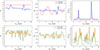 |
Fig. 4. Same as Fig. 3, but for a sausage-like jet shape with C2 = 0.8. |
| In the text | |
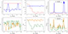 |
Fig. 5. Same as Fig. 3, but for a sausage-like jet shape with C2 = 2. |
| In the text | |
|
Fig. 6. Same as Fig. 3, but for a parabolic jet shape. The first row (single blob A) and the second row (single blob B) differ only in the initial blob coordinates. |
| In the text | |
Current usage metrics show cumulative count of Article Views (full-text article views including HTML views, PDF and ePub downloads, according to the available data) and Abstracts Views on Vision4Press platform.
Data correspond to usage on the plateform after 2015. The current usage metrics is available 48-96 hours after online publication and is updated daily on week days.
Initial download of the metrics may take a while.