| Issue |
A&A
Volume 707, March 2026
|
|
|---|---|---|
| Article Number | A55 | |
| Number of page(s) | 13 | |
| Section | Atomic, molecular, and nuclear data | |
| DOI | https://doi.org/10.1051/0004-6361/202557530 | |
| Published online | 03 March 2026 | |
The collisional excitation of CS by H2O for cometary applications
Potential energy surface, rate coefficients, and non-local thermodynamic equilibrium modeling
1
Univ. Rennes, CNRS, IPR (Institut de Physique de Rennes) – UMR 6251,
35000
Rennes,
France
2
Centro de Astrobiología (CAB, CSIC-INTA),
Ctra. de Torrejón a Ajalvir km 4,
28850
Torrejón de Ardoz, Madrid,
Spain
3
Joint Quantum Institute, Department of Physics, University of Maryland,
College Park,
MD
20742,
USA
4
Nicolaus Copernicus University in Toruń, Faculty of Chemistry,
Gagarina 7,
87-100
Toruń,
Poland
★ Corresponding authors: This email address is being protected from spambots. You need JavaScript enabled to view it.
; This email address is being protected from spambots. You need JavaScript enabled to view it.
Received:
2
October
2025
Accepted:
5
December
2025
Abstract
Aims. Collisional rate coefficients with H2O as the collisional partner for cometary applications are usually missing from the literature due to the high computational cost of such calculations. One notable example is CS, which is among the dominant sulfur-bearing species observed in comets, whose formation path remains to be elucidated.
Methods. To allow for the accurate determination of the physical conditions of comets where CS is detected, we conducted a study on the collisional excitation of CS induced by H2O.
Results. The first CS–H2O potential energy surface (PES) was computed using the symmetry adapted perturbation theory along with the density functional theory method (SAPT-DFT). The scattering calculations were performed using the statistical adiabatic channel model (SACM) approach. The rate coefficients were employed in a non-local thermodynamic equilibrium (LTE) excitation model to discuss the impact of the new data on the modeling of CS in cometary comae where H2O is dominating.
Conclusions. The first CS–H2O rate coefficients were provided for the 5–100 K temperature range, including all CS levels up to jCS = 18. It was found that using CS–H2 rate coefficients or the global cross-section approach to supplement for missing CS–H2O data are not expected to perform well. Among all approximations, using CO–H2O rate coefficients – CO being chemically similar to CS – is expected to be the most accurate approximation. Computing collisional rate coefficients with H2O projectiles to address the lack of cometary data is a highly demanding task. In this work we used the SACM approach to compute the CS–H2O data, opening the way for further calculations for cometary applications. Further testing of the impact of the approximations used to compensate for this absence in the analysis of cometary observations is required to draw strong conclusions about the inaccuracies they may introduce.
Key words: astrochemistry / molecular data / molecular processes / scattering / comets: general
© The Authors 2026
 Open Access article, published by EDP Sciences, under the terms of the Creative Commons Attribution License (https://creativecommons.org/licenses/by/4.0), which permits unrestricted use, distribution, and reproduction in any medium, provided the original work is properly cited.
This article is published in open access under the Subscribe to Open model. This email address is being protected from spambots. You need JavaScript enabled to view it. to support open access publication.
1 Introduction
Comets are thought to be remnants of planet formation and preserve valuable clues about the origin of our Solar System (Mumma & Charnley 2011). These objects may have played a role in delivering organic molecules that acted as building blocks of life on Earth. The nucleus of a comet is composed of rock surrounded by ices, consisting primarily of H2O but also of CO and CO2. As the comet approaches the Sun, these ices sublimate due to increasing solar radiation, forming an atmosphere around the nucleus known as the cometary coma. For comets at short heliocentric distances (rh ~ 1 a.u.), the surface temperature driven by solar radiation exceeds the H2O sublimation temperature, making water the dominant species in the coma.
In the coma, the density goes from 1012 cm−3 close to the surface of the nucleus to 1 cm−3 in the outer coma (Despois et al. 2006). At intermediate nucleocentric distances, the density is neither high enough for local thermodynamic equilibrium (LTE) conditions to prevail nor low enough for the fluorescence regime to be achieved. This can lead to strong non-LTE signatures in the molecular lines (Bodewits et al. 2022). Hence, the competition between radiative and collisional (de-)excitation processes must be accounted for, and thus collisional rate coefficients are required. As most cometary observations are performed on comets at short heliocentric distances (rh ~ 1 a.u.), where the molecular outgassing from the comet is the highest, the collisional rate coefficients with H2O as a collisional partner are therefore primarily required.
The determination of collisional rate coefficients is recognized as a challenging task, and it is mostly carried out using numerical calculations involving rare gases and light molecules such as H2 for interstellar applications. Since water has a relatively high mass compared to these colliders and possesses a large dipole moment, the number of channels required to achieve convergence in the calculations makes the use of quantum approaches unfeasible. Alternative methods are necessary. Currently, among over 50 molecules detected in comets through remote observations (Biver et al. 2022), collisional data with the H2O projectile exist for four molecules only. The most recent sets of collisional rate coefficients are CO–H2O by Loreau et al. (2018a); Faure et al. (2020), HF–H2O by Loreau et al. (2020, 2022), H2O–H2O data by Mandal & Babikov (2023b,a), and HCN–H2O by Żółtowski et al. (2025).
In these studies, the scattering calculations were performed using two scattering approaches: the mixed quantum classical trajectory [MQCT, Semenov & Babikov (2013); Mandal et al. (2024)] for the H2O–H2O data, and the statistical adiabatic channel model [SACM, Loreau et al. (2018b)] approaches for the other three systems. Both approaches are complementary: MQCT relies on classical mechanics and is therefore inherently more accurate at high temperatures. It has demonstrated an acceptable accuracy down to 100 K according to the work of Joy et al. (2024). SACM relies on statistical theory and is thus inherently more accurate at low temperatures. It has been shown to provide accurate results up to 100 K by Loreau et al. (2018a) in their study of CO–H2O rate coefficients.
The SACM approach employed in this work was initially proposed by Quack & Troe (1974, 1975) to treat inelastic and reactive collisions. It assumes that the complex formed by the two colliders lives long enough for the total energy of the collision to be statistically redistributed. The method operates under the straightforward assumption that all energetically accessible channels1 have equal probabilities, while all others have zero probability. Loreau et al. (2018b) refined this approach by accurately computing the adiabatic states corresponding to each channel, rather than relying on simple analytical formulas.
CS is one of the most abundant sulfur-bearing species detected in comets (Biver et al. 2022), and it has been clearly identified as a daughter molecule – meaning that it is produced by the photolysis of a species directly outgassing from the nucleus (Roth et al. 2021b). However, its parent molecule remains unidentified. CS2 was initially proposed as a possible parent molecule, but it was later found to have a lifetime that is too short and an abundance that is too low for it to be at the origin of CS formation (Calmonte et al. 2016; Roth et al. 2021b; Biver et al. 2022). Recently, Biver et al. (2024) reported that the photodissociation rate of H2CS closely matches the rate previously estimated for the parent molecule of CS, supporting the hypothesis that H2CS could be a plausible parent of CS in cometary comae. However, H2CS is also too scarce to be a likely parent. Therefore, no suitable candidate for the parent molecule of CS currently exists.
In this work, we determined the collisional rate coefficients characterizing the inelastic collisions ![Mathematical equation: $\[\mathrm{CS}\left(j_{\mathrm{CS}}\right)+\mathrm{H}_{2} \mathrm{O}\left(j_{k_{a} k_{c}}\right) \rightarrow \mathrm{CS}\left(j_{\mathrm{CS}}^{\prime}\right)+\mathrm{H}_{2} \mathrm{O}\left(j_{k_{a}^{\prime} k_{c}^{\prime}}^{\prime}\right)\]$](/articles/aa/full_html/2026/03/aa57530-25/aa57530-25-eq1.png) from 5 to 100 K for cometary applications. For that purpose, the CS–H2O potential energy surface (PES) characterizing the electronic interaction between the colliders was computed using the SAPT-DFT. The scattering calculations were performed based on the computed PES using the SACM approach. The rate coefficients were computed by including all transitions between CS levels up to jCS ≤ 18 (279.44 cm−1), and para-H2O (hereafter, noted p-H2O) levels up to the jkakc ≤ 220 (136.56 cm−1), and ortho-H2O (hereafter, noted o-H2O) levels up to jkakc ≤ 303 (136.91 cm−1). The new CS–H2O of rate coefficients have been employed in non-LTE excitation models, alongside CS–H2 rate coefficients and the rate coefficients derived by Biver et al. (1999). The latter are derived based on a global cross section. The objective is to assess the impact of the different datasets on the excitation conditions of CS in comets. This paper also includes a discussion of the expected accuracy of the CS–H2O data and proposes guidelines for which approximations can be used to accurately model the excitation of molecules in comets when collisional rate coefficients with H2O are unavailable. Finally, conclusions are presented.
from 5 to 100 K for cometary applications. For that purpose, the CS–H2O potential energy surface (PES) characterizing the electronic interaction between the colliders was computed using the SAPT-DFT. The scattering calculations were performed based on the computed PES using the SACM approach. The rate coefficients were computed by including all transitions between CS levels up to jCS ≤ 18 (279.44 cm−1), and para-H2O (hereafter, noted p-H2O) levels up to the jkakc ≤ 220 (136.56 cm−1), and ortho-H2O (hereafter, noted o-H2O) levels up to jkakc ≤ 303 (136.91 cm−1). The new CS–H2O of rate coefficients have been employed in non-LTE excitation models, alongside CS–H2 rate coefficients and the rate coefficients derived by Biver et al. (1999). The latter are derived based on a global cross section. The objective is to assess the impact of the different datasets on the excitation conditions of CS in comets. This paper also includes a discussion of the expected accuracy of the CS–H2O data and proposes guidelines for which approximations can be used to accurately model the excitation of molecules in comets when collisional rate coefficients with H2O are unavailable. Finally, conclusions are presented.
2 Numerical methods
2.1 Ab initio calculations
We developed a new ab initio PES for the scattering calculations between the CS and H2O colliders. We considered CS and H2O molecules as rigid with their geometries corresponding to the ground electronic and rovibrational states. The CS interatomic distance was fixed at 2.9179a0 and r(OH) bond distances in the H2O molecule were fixed at 1.8368a0 with the HOH angle of 104.7 degrees. This leads to the five-dimensional PES; namely, the interaction is completely described by one radial (R) and four angular coordinates.
We followed the recent work of Dagdigian (2020) to set up the origin of the coordinate system in the center of mass (c.o.m.) of the H2O monomer. With this choice, the V(R, θ1, ϕ1, θ2, ϕ2) PES describes the position of the c.o.m. of the CS molecule around the H2O monomer with a Jacobi vector, R, which has (R, θ1, ϕ1) spherical coordinates. (R, θ1, ϕ1) has its origin on the H2O c.o.m., with R being the intermolecular distance between the c.o.m.s of H2O and CS and the pair of angles (θ1, ϕ1) describing the angular position of the c.o.m. of the CS molecule. The remaining spherical angles (θ2, ϕ2) describe the relative orientation of the CS rotor with respect to an H2O fixed system of coordinates, which has a z axis coincidental with the C2 symmetry axis of the water molecule and in which the water molecule lies on the xz plane.
To determine the PES, we used the SAPT(DFT) (Misquitta & Szalewicz 2005; Misquitta et al. 2005) with the augmented correlation-consistent quadruple-zeta basis set (aug-cc-pVQZ). The PES was generated using the AUTOPES package (Metz et al. 2016). In this approach, the short-range part of the interaction is obtained by partitioning the system into two monomers (H2O and CS in our case) and evaluating the electrostatic, exchange, induction, and dispersion energies together with their exchange counterparts (exchange–induction and exchange–dispersion). In addition, the ![Mathematical equation: $\[\delta E_{\text {int,resp}}^{\mathrm{HF}}\]$](/articles/aa/full_html/2026/03/aa57530-25/aa57530-25-eq2.png) correction (Patkowski et al. 2006) was included in the final SAPT-DFT PES to account for higher-order induction and exchange–induction effects. The long-range part was constructed independently from monomer electron densities and frequency-dependent density susceptibility functions at the coupled Kohn–Sham level, leading to a c.o.m.–c.o.m. asymptotic multipole expansion of the interaction energy in inverse powers of R. The two parts are then smoothly merged into a global PES, which is built by freezing the damped asymptotic part and fitting only the short-range term, which produces a smooth potential (Metz et al. 2016). The resulting surface reproduces the interaction energies with root-mean-square (RMS) errors of 2.5 cm−1 for energies below −600 cm−1, 18 cm−1 along the repulsive wall up to 3500 cm−1, 4.5 cm−1 for all bound configurations (energies below 0), and 57 cm−1 for highly repulsive configurations near 35 000 cm−1. Those errors are not expected to significantly impact the scattering calculations, considering that they are marginal with respect to both the well depth of the system and the accuracy of the SACM method.
correction (Patkowski et al. 2006) was included in the final SAPT-DFT PES to account for higher-order induction and exchange–induction effects. The long-range part was constructed independently from monomer electron densities and frequency-dependent density susceptibility functions at the coupled Kohn–Sham level, leading to a c.o.m.–c.o.m. asymptotic multipole expansion of the interaction energy in inverse powers of R. The two parts are then smoothly merged into a global PES, which is built by freezing the damped asymptotic part and fitting only the short-range term, which produces a smooth potential (Metz et al. 2016). The resulting surface reproduces the interaction energies with root-mean-square (RMS) errors of 2.5 cm−1 for energies below −600 cm−1, 18 cm−1 along the repulsive wall up to 3500 cm−1, 4.5 cm−1 for all bound configurations (energies below 0), and 57 cm−1 for highly repulsive configurations near 35 000 cm−1. Those errors are not expected to significantly impact the scattering calculations, considering that they are marginal with respect to both the well depth of the system and the accuracy of the SACM method.
Additionally, we performed benchmark calculations employing the “gold standard” of electronic structure methods, the coupled cluster method with single, double, and non-iterative triple excitations with explicit correlation [CCSD(T)-F12], using the augmented correlation-consistent triple-zeta basis set (aug-cc-pVTZ) supplemented with mid-bond functions for selected cuts of the PES. A good agreement was found between the SAPT(DFT) and CCSD(T)-F12 PESs. In Fig. 1 we show the comparison of the SAPT-DFT fit to selected cuts from our calculations with the gold standard CCSD(T)-F12 method. We note that the CCSD(T)-F12 calculations are more computationally demanding than SAPT(DFT) calculations, especially to scan five angular dimensions. For the relative orientation of CS and H2O near the global minimum (geometry labeled “C” in Fig. 1), the CCSD(T)-F12 PES gives the well depth of 1269.6 cm−1 at R = 8.07a0, which is only about 50 cm−1 deeper (4% relative difference) than the SAPT-DFT minimum. This difference in the global minimum well depth is mainly due to the inclusion of the perturbative triple excitations in the CCSD(T)-F12 method. We found by computing interaction energies without mid-bond functions that the bond functions contribute about 3.4 cm−1 to the global minimum for the arrangement C shown in Fig. 1. For arrangements A and B, the mid-bond functions contribute on a similar order, about 5 cm−1, which is about 1–2% of the interaction energy at minima of these arrangements. The CCSD(T)-F12 method with triple-zeta basis and mid-bond functions provides in practice interaction energies close to the complete basis set limit.
The next step after completion of the electronic structure calculations of the PES is to represent the potential as an expansion in the tensor spherical functions used in HIBRIDON program. We followed the work of Dagdigian (2020) for this step and we refer the reader to this reference for details of the angular expansion. The only difference is that Dagdigian (2020) considered H2 as a collider, which limits the rotational quantum number, l2, of the spherical rotor function in the potential expansion to being evenvalued, which is not the case for our CS molecule, where both spherical rotor functions with odd and even-valued l2 are necessary. We expanded the PES to include expansion coefficients up to l1 = 10, l2 = 6, and l = 6. The expansion of the SAPT-DFT PES in those terms results in the following RMS errors: at the distance R = 5a0, the RMS is 128 cm−1 for interaction energies ranging from 103 to 104 cm−1; while at R = 8.1a0 (near the Re of the PES), the RMS is 2.7 cm−1 for energies ranging from - 1100 cm−1 to 900 cm−1. Finally, for the intermediate (R = 10a0, and energy range from −500 cm−1 to 300 cm−1) and longer range (R = 20a0, and an energy range from −30 cm−1 to 30 cm−1), the RMSs are 0.33 cm−1 and 0.001 cm−1, respectively. We conclude that this expansion provides a good description of the PES for our purpose without the significant increase in computational time that larger expansion sets may pose.
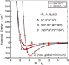 |
Fig. 1 Comparison of the CS–H2O SAPT(DFT) and aVQZ PES fit (solid black line) with the CCSD(T)-F12 and aVTZ+BF calculations performed for selected radial cuts. The θ1 and ϕ1 are spherical angles of the R vector, while θ2 and ϕ2 are spherical angles describing the orientation of the CS molecule. |
2.2 Scattering calculations
To obtain all of the information about the collision, the scattering matrices, denoted as ![Mathematical equation: $\[S_{\gamma, \gamma^{\prime}}^{J}(E) ~(\gamma^{\prime \prime} \equiv j_{\mathrm{CS}}^{\prime \prime} j^{\prime \prime} k_{a}^{\prime \prime} k_{c}^{\prime \prime} j_{12}^{\prime \prime} l^{\prime \prime})\]$](/articles/aa/full_html/2026/03/aa57530-25/aa57530-25-eq3.png) , were calculated for each total angular momentum J. The SACM approach starts with the same equations then the close-coupling (hereafter, CC) approach, expressed as follows (Alexander et al. 2023):
, were calculated for each total angular momentum J. The SACM approach starts with the same equations then the close-coupling (hereafter, CC) approach, expressed as follows (Alexander et al. 2023):
![Mathematical equation: $\[\left[\mathbf{I} \frac{d^2}{d R^2}+\mathbf{W}(R)\right] \mathbf{F}(R)=0,\]$](/articles/aa/full_html/2026/03/aa57530-25/aa57530-25-eq4.png) (1)
(1)
with the identity matrix, I, the radial part of the wavefunction, F(R), and the W(R) matrix defined as
![Mathematical equation: $\[\mathbf{W}(R)=\mathbf{k}^2-\mathbf{l}^2-\frac{2 \mu}{\hbar^2} \mathbf{V}(R),\]$](/articles/aa/full_html/2026/03/aa57530-25/aa57530-25-eq5.png) (2)
(2)
with μ the reduced mass of the collisional system. V(R) is the matrix of the coupling potential, and k and l are diagonal matrix of the wavevector and of the relative angular momentum of the collisional partners, defined, respectively, as
![Mathematical equation: $\[k_{i i}^2=\frac{2 \mu}{\hbar^2}\left(E-\epsilon_i\right),\]$](/articles/aa/full_html/2026/03/aa57530-25/aa57530-25-eq6.png) (3)
(3)
![Mathematical equation: $\[l_{i i}^2=\frac{\hbar^2}{2 \mu R^2} l_i\left(l_i+1\right),\]$](/articles/aa/full_html/2026/03/aa57530-25/aa57530-25-eq7.png) (4)
(4)
with ℏ the Planck constant divided by 2π, ϵi the energy of the channel, i, and li the relative orbital angular momentum of the ith channel. The diagonalization of the V(R) + l2 matrix yields the diagonal matrix of adiabatic wavevectors, which define the locally adiabatic states.
To study the inelastic CS–p-H2O and CS–o-H2O collisions using the SACM approach, we computed the adiabatic states of the system by diagonalization of the potential matrix, V(R), including the relative angular momentum matrix, l2, following the work of Loreau et al. (2018a). A probability was then assigned to the channels – based on whether they are open or closed – to construct the ![Mathematical equation: $\[S_{\gamma, \gamma^{\prime}}^{J}(E)\]$](/articles/aa/full_html/2026/03/aa57530-25/aa57530-25-eq8.png) matrices. For a channel to be open, it must be energetically accessible at the total energy of the system, E. It means that its adiabatic state must present a minimum, and that its energy between the minima and its asymptotic value must always be lower than E. A closed channel is one that does not meet one of these requirements. The SACM approach works under the straightforward assumption that all open channels has the same probability,
matrices. For a channel to be open, it must be energetically accessible at the total energy of the system, E. It means that its adiabatic state must present a minimum, and that its energy between the minima and its asymptotic value must always be lower than E. A closed channel is one that does not meet one of these requirements. The SACM approach works under the straightforward assumption that all open channels has the same probability, ![Mathematical equation: $\[\frac{1}{N}\]$](/articles/aa/full_html/2026/03/aa57530-25/aa57530-25-eq9.png) , with N the total number of open channels, while any closed channel has zero probability. Additional details of the method can be found in Loreau et al. (2018b,a), Żółtowski et al. (2025), Godard Palluet et al. (2025), and Tonolo et al. (2025).
, with N the total number of open channels, while any closed channel has zero probability. Additional details of the method can be found in Loreau et al. (2018b,a), Żółtowski et al. (2025), Godard Palluet et al. (2025), and Tonolo et al. (2025).
From these ![Mathematical equation: $\[S_{\gamma, \gamma^{\prime}}^{J}(E)\]$](/articles/aa/full_html/2026/03/aa57530-25/aa57530-25-eq10.png) matrices, the inelastic cross sections were finally computed as
matrices, the inelastic cross sections were finally computed as
![Mathematical equation: $\[\sigma_{\gamma \rightarrow \gamma^{\prime}}(E)=\frac{\pi}{g_1 g_2 k_{\gamma, \gamma^{\prime}}^2} \sum_J(2 J+1) \sum_{l l^{\prime}}\left|S_{\gamma, \gamma^{\prime}}^J(E)\right|^2,\]$](/articles/aa/full_html/2026/03/aa57530-25/aa57530-25-eq11.png) (5)
(5)
with gi the degeneracy of the rotational state of monomer i, and ![Mathematical equation: $\[k_{\gamma, \gamma^{\prime}}^{2}=\frac{2 \mu}{\hbar^{2}}\left(E-E_{\gamma}\right)\]$](/articles/aa/full_html/2026/03/aa57530-25/aa57530-25-eq12.png) the wavenumber.
the wavenumber.
The state-to-state rate coefficients at a given kinetic temperature, Tk, were obtained by calculating the thermal average of the cross sections over kinetic energies
![Mathematical equation: $\[k_{\gamma \rightarrow \gamma^{\prime}}\left(T_k\right)=\sqrt{\frac{8}{\pi \mu k_B^3 T_k^3}} \int \sigma_{\gamma \rightarrow \gamma^{\prime}}\left(E_k\right) E_k ~\exp \left(\frac{-E_k}{k_B T_k}\right) d E_k,\]$](/articles/aa/full_html/2026/03/aa57530-25/aa57530-25-eq13.png) (6)
(6)
where Ek = E − Eγ is the kinetic energy of the transition.
With this approach, the computational cost is drastically reduced for three reasons:
The determination of the adiabatic states does not require a R grid as thin or as large as for the propagation of F(R), which is the matrix defining the expansion coefficients. Indeed, only the region between the minimum and the centrifugal barrier region must be accurately described; the long-range interaction will not impact the adiabatic counting.
The convergence of the cross sections does not require the inclusion of asymptotically closed channels in the calculation of V(R) and l2 matrix elements, contrary to quantum approaches such as CC or the coupled-state approximation. Thus, a much smaller rotational basis can be used, significantly reducing the computational cost.
The adiabatic states are independent of the total energy, E, so they are computed once per J. Only the adiabatic channel counting – the least expensive part of these calculations – needs to be performed at each energy.
The central processing unit (CPU) time required for both CC and SACM approaches is proportional to ![Mathematical equation: $\[N_{c h}^{3}\]$](/articles/aa/full_html/2026/03/aa57530-25/aa57530-25-eq14.png) (Nch being the number of channels). Therefore, if Nch is reduced by a factor of 5 with the SACM method, the CPU time will be reduced by a factor of 53. An additional factor will also saved considering that the adiabatic states are valid at all energies.
(Nch being the number of channels). Therefore, if Nch is reduced by a factor of 5 with the SACM method, the CPU time will be reduced by a factor of 53. An additional factor will also saved considering that the adiabatic states are valid at all energies.
In this work the goal was to compute rate coefficients characterizing the ![Mathematical equation: $\[\mathrm{CS}\left(j_{\mathrm{CS}}\right)+\mathrm{H}_{2} \mathrm{O}\left(j_{k_{a} k_{c}}\right) \rightarrow \mathrm{CS}\left(j_{\mathrm{CS}}^{\prime}\right)+\mathrm{H}_{2} \mathrm{O}\left(j_{k_{a}^{\prime} k_{c}^{\prime}}^{\prime}\right)\]$](/articles/aa/full_html/2026/03/aa57530-25/aa57530-25-eq15.png) inelastic collisions for temperatures from 5 to 100 K. The rate coefficients thus include transitions involving CS rotational levels of up to jCS ≤ 18, and the first five levels of p– and o-H2O, up to jkakc ≤ 220 for p-H2O, and up to jkakc ≤ 303 for o-H2O.
inelastic collisions for temperatures from 5 to 100 K. The rate coefficients thus include transitions involving CS rotational levels of up to jCS ≤ 18, and the first five levels of p– and o-H2O, up to jkakc ≤ 220 for p-H2O, and up to jkakc ≤ 303 for o-H2O.
The rotational constants of water were taken from Herzberg (1966), with A = 27.877 cm−1, B = 14.512 cm−1, and C = 9.285 cm−1 the rotational constants corresponding to the moments of inertia along the a, b, and c axes, respectively, with Ia ≠ Ib ≠ Ic. The rotational constant of CS was taken as BCS = 0.817 cm−1 according to Bustreel et al. (1979).
The adiabatic states were computed using the HIBRIDON software (Alexander et al. 2023). To reduce the computational cost, the number of channels was limited by using both the EMAX parameter and the rotational basis. The EMAX option will remove from the basis any channels with an energy greater than EMAX2. As the convergence of the cross sections is weakly sensitive to asymptotically closed channels within the SACM approach, using this option will not impact the precision of the results, but will reduce the computational time. The rotational basis was finally restricted to jCS ≤ 31 and jkakc ≤ 3kakc for CS–p-H2O, and to jCS ≤ 26 and jkakc ≤ 3kakc for CS–o-H2O to reduce computational cost while maintaining the precision of the rate coefficients. The EMAX parameter was set at 817 cm−1, the highest total energy considered in the scattering calculations. The convergence of the rotational basis and of the EMAX parameter for the adiabatic state calculations, along with additional information about the calculations, is presented in Appendix A.
The cross sections were then calculated following the SACM approach described above, and summed over an increasing number of partial waves, J, until a convergence of the cross sections at better than 5% was observed. As a result, partial waves with 0 ≤ J ≤ 153 were included for the calculation of CS–p-H2O cross sections, and with 0 ≤ J ≤ 149 for the CS–o-H2O cross sections. By averaging the cross sections over a thermal distribution of the kinetic energies, the state-to-state rate coefficients were obtained from Eq. (6).
2.3 Non-LTE modeling
To evaluate the influence of the new rate coefficients on the interpretation of cometary observations, we incorporated the CS–H2O rate coefficients into a non-LTE excitation model to simulate the population of CS energy levels at various nucleocentric distances within the coma. The corresponding gas density was evaluated using the Haser (1957) model as follows:
![Mathematical equation: $\[n_{\mathrm{H}_2 \mathrm{O}}(r)=\frac{Q_{\mathrm{H}_2 \mathrm{O}}}{4 \pi r^2 v_{exp }} ~\exp \left(-r \frac{\beta_{\mathrm{H}_2 \mathrm{O}}}{v_{exp }}\right),\]$](/articles/aa/full_html/2026/03/aa57530-25/aa57530-25-eq16.png) (7)
(7)
with nH2O the density of water vapor as a function of the nucleocentric distance, r, and βH2O = 1.042 × 10⁻⁵ s−1 the photodissociation rate of water taken from Zakharov et al. (2007). QH2O, the production rate of water, was set at 1029 cm−3 s−1. vexp, the expansion velocity of the gas, was set at 1 km s−1. The value of the production rates and the expansion velocity was settled in order to represent the “average” water-dominated comet at a heliocentric distance of rh = 1 a.u. (Bodewits et al. 2022), following the methodology set out in Lupu et al. (2007) and Faure et al. (2020).
The population of CS energy levels at different nucleocentric distances was determined by solving the coupled radiative transfer equations and statistical equilibrium equations using the escape probability formalism as implemented in the RADEX code developed by van der Tak et al. (2007). The nucleocentric distances were considered between 102 and 106 km. The kinetic temperature of the gas was set at 100 K.
In comets, CS represents between 0.03 and 0.2% of cometary volatiles, and CO represents on average about 10% (Biver et al. 2022). Therefore, the column density of CS, denoted as NCS, was set at 1 × 1012 cm−2, so 1% of the CO column density reported by Lupu et al. (2007), who estimated a CO column density of approximately 1 × 1014 cm−2 at a nucleocentric distance of r ≃ 103 km in a water-dominated comet at an heliocentric of rh ~ 1 a.u3.
The linewidth was set at δν = 2vexp. The background radiation field was considered as the combination of the cosmic microwave background radiation field at 2.73 K and the solar radiation field. The latter was considered as a blackbody of 5770 K diluted with the corresponding factor W = ΩS/4π, where ΩS ≃ 6.79 × 10⁻⁵ sr is the solid angle of the Sun at a heliocentric distance, rh, of 1 a.u. The Einstein coefficients were taken from the Cologne Database for Molecular Spectroscopy (Müller et al. 2001, 2005; Endres et al. 2016).
The RADEX code requires thermalized rate coefficients, which were computed from the state-to-state rate coefficients by assuming a thermal distribution of o/p-H2O as
![Mathematical equation: $\[k_{j_{\mathrm{CS}} \rightarrow j_{\mathrm{CS}}^{\prime}}(T)=\sum_{j_{k_a k_c}} n_{j_{k_a k_c}}(T) \sum_{j_{k_a^{\prime} k_c^{\prime}}^{\prime}} k_{\gamma \rightarrow \gamma^{\prime}}(T),\]$](/articles/aa/full_html/2026/03/aa57530-25/aa57530-25-eq17.png) (8)
(8)
with njkakc (T) the population of the jkakc level at the kinetic temperature, T:
![Mathematical equation: $\[n_{j_{k_a k_c}}(T)=\frac{(2 j+1) ~\exp \left(\frac{-E_{j_{k_a k_c}}}{k_B T}\right)}{\sum_{j^{\prime}_{k_a^{\prime} k_c^{\prime}}}\left(2 j^{\prime}+1\right) ~\exp \left(\frac{-E_{j^{\prime}_{k_a^{\prime} k_c^{\prime}}}}{k_B T}\right)}.\]$](/articles/aa/full_html/2026/03/aa57530-25/aa57530-25-eq18.png) (9)
(9)
The thermalized rate coefficients were used by assuming an o/p ratio of three, which is a typical value observed in comets at a kinetic temperature higher than 50 K (Biver et al. 2022).
This model is a very simplified one compared to the complex processes taking place in the coma: the chemistry of CS is neglected, as is the effect of the heliocentric distance on the abundance of CS, the impact of electrons, and the excitation of CS vibrational states by solar radiation. The objective of this model is to capture collisional effects, and we do not intend to predict any quantitative data from this model. For the accurate interpretation of observational molecular spectra of CS, more sophisticated approaches exist, such as the SUBLIME code described in Cordiner et al. (2023).
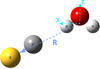 |
Fig. 2 Global minimum equilibrium geometry of the CS–H2O SAPT(DFT) and aVQZ PES. The Re between the c.o.m. of H2O and c.o.m. of CS is 8.11a0, with θ1 = 122°, θ2 = 297°, and ϕ1 = ϕ2 = 0°. |
3 Results
3.1 Potential energy surface
The analysis of the fitted SAPT(DFT) PES reveals two minima. In Fig. 2 we show the global minimum geometry of the CS–H2O SAPT(DFT) PES. It corresponds to the configuration in which the carbon atom of the CS molecule points toward one of the hydrogen atoms of the H2O molecule, as is shown in Fig. 2, and corresponding to the minimum on curve C in Fig. 1. The c.o.m. separation is 8.11a0, the angular coordinates are θ1 = 122°, θ2 = 297°, and ϕ1 = ϕ2 = 0°, and the well depth is 1219.23 cm−1. A secondary minimum (curve marked as A in Fig. 1) is found for the geometry where the sulfur atom points toward the oxygen atom of the water molecule, with a c.o.m. separation of 7.06a0 with θ1 = θ2 = ϕ1 = ϕ2 = 0° and a well depth of 660.44 cm−1. The radial minimum for the arrangement B in Fig. 1 corresponds to the CS perpendicular to the H2O plane, with the sulfur atom pointing toward H2O. The c.o.m. separation for this minimum is R=7.36a0, with angular coordinates of θ1 = θ2 = ϕ1 = ϕ2 = 90° and a well depth of 335.44 cm−1. In Fig. 3, we show the anisotropy of the SAPT(DFT) PES for the cut showing potential as a function of θ1 and θ2 angular coordinates for a fixed R=8.11a0, with other angles fixed at ϕ1 = ϕ2 = 0°.
It can be observed that the global minima and secondary minimum are separated by a barrier at about −328 cm−1. The PES is found to be highly anisotropic with respect to both the θ1 and θ2 angles. The potential can change by about 1000 cm−1 for a rotation of θ1 smaller than 90°, and by roughly 1400 cm−1 for a 180° rotation of θ2. This shows that the interaction is very sensitive to the geometry of the complex.
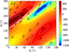 |
Fig. 3 SAPT(DFT) PES of the CS–H2O complex for varying orientation angles, θ1 and θ2, with ϕ1 = ϕ2 = 0° at R = 8.11a0. |
3.2 Rate coefficients
The behavior of the thermalized rate coefficients for CS–p-H2O and CS–o-H2O, obtained from Eq. (8) and later used in non-LTE excitation models, is shown in Fig. 4. The thermalized de-excitation rate coefficients generally decrease with increasing temperature, with a few exceptions such as the ![Mathematical equation: $\[j_{\mathrm{CS}}=4 \rightarrow j_{\text {CS }}^{\prime}=0\]$](/articles/aa/full_html/2026/03/aa57530-25/aa57530-25-eq19.png) transition exhibited in Fig. 4, where the rate coefficient slightly increases from 5 to 20 K and then decreases smoothly up to 100 K. For both p-H2O and o-H2O, the favored transitions are the ones with the minimum kinetic energy release. In other words, as
transition exhibited in Fig. 4, where the rate coefficient slightly increases from 5 to 20 K and then decreases smoothly up to 100 K. For both p-H2O and o-H2O, the favored transitions are the ones with the minimum kinetic energy release. In other words, as ![Mathematical equation: $\[\left|\Delta j_{\mathrm{CS}}\right|=\left|j_{\mathrm{CS}}^{\prime}-j_{\mathrm{CS}}\right|\]$](/articles/aa/full_html/2026/03/aa57530-25/aa57530-25-eq20.png) increases, the magnitudes of the rate coefficients are decreasing. The CS–p-H2O and CS–o-H2O rate coefficients exhibit very similar behavior. In a systematic comparison (see Fig. B.1), CS–p-H2O and CS–o-H2O rate coefficients become increasingly similar as the temperature increases. At 10 K, deviations by more than a factor of two are observed for a few transitions, whereas at 100 K, the two sets of data agree within a factor of 1.5. In previous studies on the collisional excitation of CO, HF, and HCN induced by water molecules (Faure et al. 2020; Loreau et al. 2022; Żółtowski et al. 2025), the authors already observed that the excitation rate coefficients induced by p- and o-H2O were relatively similar.
increases, the magnitudes of the rate coefficients are decreasing. The CS–p-H2O and CS–o-H2O rate coefficients exhibit very similar behavior. In a systematic comparison (see Fig. B.1), CS–p-H2O and CS–o-H2O rate coefficients become increasingly similar as the temperature increases. At 10 K, deviations by more than a factor of two are observed for a few transitions, whereas at 100 K, the two sets of data agree within a factor of 1.5. In previous studies on the collisional excitation of CO, HF, and HCN induced by water molecules (Faure et al. 2020; Loreau et al. 2022; Żółtowski et al. 2025), the authors already observed that the excitation rate coefficients induced by p- and o-H2O were relatively similar.
3.3 Excitation of CS in comets
The new sets of CS–H2O thermalized rate coefficients were employed in a non-LTE radiative transfer model to investigate non-LTE effects on CS level populations in water-dominated comae, following the methodology described in Sect. 2.3. We also examined the impact of two approximations commonly used in the literature to compensate for the lack of collisional data. Cordiner et al. (2023) used the collisional rate coefficients of CS–p-H2 and CS–o-H2, computed by Denis-Alpizar et al. (2018), as substitutes for the CS–p-H2O and CS–o-H2O rate coefficients. The second approximation was employed by Biver et al. (1999), based on the work of Bockelée-Morvan (1987) and Crovisier (1987), who derived the rate coefficients (hereafter noted B99) from a single global cross section, σc = 5 × 10⁻¹⁴, cm2, adapted from the H2O-H2O pressure broadening experiment of Murphy & Boggs (1969). The temperature-dependent rate coefficients were computed as ![Mathematical equation: $\[k_{c}(T)=\sigma_{c}~\langle v(T)\rangle n_{j_{\mathrm{CS}}^{\prime}}(T)\]$](/articles/aa/full_html/2026/03/aa57530-25/aa57530-25-eq21.png) , with ⟨v(T)⟩ being the mean velocity at the kinetic temperature, T, of the medium, and
, with ⟨v(T)⟩ being the mean velocity at the kinetic temperature, T, of the medium, and ![Mathematical equation: $\[n_{j_{\mathrm{CS}}^{\prime}}(T)\]$](/articles/aa/full_html/2026/03/aa57530-25/aa57530-25-eq22.png) being the population of the final CS level, assuming a Boltzmann distribution. In their approach, they do not differentiate between ortho and para water, and the rate coefficients inferred from this approximation are independent of the initial level.
being the population of the final CS level, assuming a Boltzmann distribution. In their approach, they do not differentiate between ortho and para water, and the rate coefficients inferred from this approximation are independent of the initial level.
In Fig. 5, we represent the populations of CS energy levels involved in the most frequently observed transitions – namely, j = 3 → 2, 5 → 4, and 7 → 6 (Roth et al. 2021a; Cordiner et al. 2023; Biver et al. 2023, 2024) – as a function of the nucleocentric distance, r. Therefore, the deviations observed in the populations are expected to be the ones most significantly affecting the modeling of CS emission spectra from the coma.
According to Fig. 5, the population of CS energy levels as a function of nucleocentric distance can be divided into three categories. Region (a) corresponds to the LTE domain, spanning distances from a few to a few hundred kilometers. This region represents the inner coma, where the density is high and molecular excitation is dominated by collisions. As a result, the CS level populations follow a Boltzmann distribution. Region (b) corresponds to the non-LTE domain, extending from a few hundred kilometers to approximately 105 km from the nucleus. As the distance from the nucleus increases, the density decreases, and the population of CS energy levels deviates significantly from LTE conditions. Region (c) defines the fluorescence domain, where the excitation of CS is primarily governed by solar radiation. This corresponds to the outer part of the coma, where the density is so low that collisions can be neglected, as they no longer significantly affect the population of CS energy levels.
For single-dish observations, the telescope beam sizes are typically larger than a few arc-seconds, corresponding to nucleocentric distances greater than 103 km for a comet at a geocentric distance of 1 a.u. (Bodewits et al. 2022). Therefore, the beam will necessarily include regions beyond the LTE domain (which, according to this study, extends to approximately 102 km), meaning that non-LTE modeling is required to accurately derive CS production rates in comets.
In Fig. 5, we also show the population of CS energy levels when CS–H2 rate coefficients are used instead of CS–H2O coefficients. We observe that the CS level populations differ significantly in the mid-coma region – where non-LTE effects are prominent – depending on which set of rate coefficients is used. Differences of over a factor of two can be observed between the populations, which can have a substantial impact on the modeling of CS production rates. This is not surprising, as a systematic comparison of state-to-state rate coefficients shows that CS–H2O rate coefficients are significantly different than those of CS–H2, by up to three orders of magnitude for the weakest transitions (see Fig. C.1). With CS–H2O rate coefficients, the population of CS energy levels thermalizes at lower densities (i.e., at larger nucleocentric distances) due to more efficient energy transfer through collisions. This is due to the larger dipole moment of H2O compared to H2, resulting in stronger interactions with the target molecule, and so larger rate coefficients (see Fig. C.1).
In Fig. 5, we also show the population of CS energy levels using the set of B99 rate coefficients. The differences observed between the populations evaluated with the accurate CS–H2O rate coefficients (computed in this work) and those obtained using the B99 datasets are very significant, and they can be by a factor of three. Thus, the use of B99 datasets is expected to lead to strong inaccuracies in the determination of the physical conditions within the coma.
We observe that the populations thermalize at slightly higher nucleocentric distances (i.e., lower densities), suggesting that the efficiency of collisions is overestimated with this approach. This is confirmed by the comparison between B99 and CS–H2O rate coefficients, exhibited in Fig. D.1, where B99 data are generally greater than CS–H2O data, and some transitions can be overestimated by over two orders of magnitudes at 100 K. Therefore, the analysis based on either approximation (using CS–H2 or B99 datasets) should be revised, as using the accurate sets of data could lead to significant revision of CS production rates in comets.
In the work of Faure et al. (2018) on the excitation of CO by H2O, only small differences were found between the CO populations derived using the accurate CO–H2O dataset and those obtained with the global cross-section approximation of Biver et al. (1999) at 100 K. On the other hand, in the study on the excitation of HF by H2O by Loreau et al. (2022), this approximation led to differences of up to a factor of 3 between the populations of HF obtained with the HF–H2O rate coefficients they computed and one derived from the global cross sections employed by Bockelée-Morvan et al. (2014). Therefore, it remains uncertain on which collisional systems this approximation is expected to perform well, and it thus should be used with care.
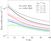 |
Fig. 4 Representation of de-excitation thermalized rate coefficients (in cm3 s−1) of the CS–p-H2O (solid lines) and CS–o-H2O (dashed lines) from the first rotationally excited states (j1 = 1, 2, 3, 4) to the ground rotational state (j = 0). |
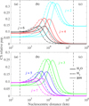 |
Fig. 5 Population of CS energy levels (2 ≤ jCS ≤ 7) as a function of the nucleocentric distance (in km) using CS–H2O thermalized rate coefficients computed in this work (solid lines) and CS–H2 thermalized rate coefficients (dash-dotted lines) at 100 K. The range of nucleocentric delimits the following zones: (a) inner-coma, LTE; (b) mid-coma non-LTE; (c) outer coma fluorescence. Odd and even jCS have been separated for the sake of clarity. |
4 Discussion
4.1 The expected accuracy of the CS–H2O rate coefficients
To properly assess the accuracy of the CS–H2O rate coefficients provided in this work, a comparison with experimental or with quantum CC calculations should be performed. As far as the authors are aware, no experimental measurements have been carried out on the CS–H2O system, either of cross sections using crossed-beam experiments, or of rate coefficients, using double-resonances techniques for example. Regarding the CC calculations, the CS–H2O system has a very deep potential well around 1200 cm−1, meaning that many channels are coupled in the well, and thus that many closed channels are necessary to converge CC cross sections (this is also true with the coupled-states approximation). Therefore, it was not possible to converge transitions for the CS–H2O system using the CC approach.
Another way to estimate the accuracy of the CS–H2O rate coefficients is to compare the performance of SACM-derived rate coefficients for similar systems, for which comparisons with experimental or CC rate coefficients are available. The most suitable comparison system is CO–H2O, as it has the same number of valence electrons, and its PES shares many similarities with that of CS–H2O, particularly in the geometry of the global minimum – indicating similar chemical behavior.
For the calculation of the CO–H2O rate coefficients, Loreau et al. (2018a) computed rate coefficients with the SACM method over the temperature range 5–100 K. The PES exhibits a global minimum around 650 cm−1 – approximately half as deep as the minimum of the CS–H2O PES, which lies at ~1200 cm−1. As a result, the lifetime of the CO–H2O complex is expected to be shorter than that of CS–H2O. In addition, the number of available channels is significantly higher for CS–H2O, as CS is heavier than CO. Therefore, the CS–H2O intermediate complex is expected to exhibit a longer lifetime and a distribution of exit channels that more closely follows statistical behavior. Consequently, the SACM approach is expected to yield greater accuracy when applied to CS–H2O collisions than to CO–H2O. Loreau et al. (2018a) evaluated the accuracy of SACM cross sections by comparing them with full CC cross sections, limited to a few partial waves, J = 0–3, due to computational constraints4. They estimated that the SACM rate coefficients were accurate to within a factor of 1.5. Therefore, at least this level of accuracy – if not better – can be expected for the CS–H2O rate coefficients presented in this work.
4.2 In the absence of cometary data: alternative strategies
In contexts in which collisional rate coefficients are unavailable – as in cometary atmospheres, where only five molecules (CO, HF, H2O, HCN, and now CS) can be studied using non-LTE models with appropriate sets of rate coefficients – it is important to assess the accuracy of alternative strategies used to address this limitation. The following strategies can be employed to compensate for the lack of available rate coefficients in excitation models:
Deriving rate coefficients based on a global cross sections derived from pressure-broadening experiments (Bockelée-Morvan 1987; Crovisier 1987).
Using interstellar rate coefficients (with H2 as a collider) to replace cometary ones (with CO, CO2, or H2O colliders, e.g., Cordiner et al. 2022, 2023)5.
Using rate coefficients involving other molecules based on the assumption that the collisional systems are similar enough (e.g., Cernicharo et al. 2024).
The first approximation is specific to the study of cometary comae and is widely used in contexts in which almost no collisional data exist. However, its impact on the derived physical parameters remains unknown. The second approximation assumes that excitation by light colliders (such as H2) is presumably similar to that by heavier colliders (e.g., H2O or CO). The final approximation is based on the assumption that if two molecules are sufficiently similar, their rate coefficients should also be similar. This approximation has been previously employed for interstellar applications (e.g., OCS–H2 for HNCS–H2 in Cernicharo et al. 2024), where the selection is based on data availability and similarities in the rotational structure between the two species. The impact of these approximations must be discussed in order to provide guidelines for cases in which rate coefficients are not available.
It was shown in the previous section that using either CS–H2 or B99 rate coefficients instead of CS–H2O rate coefficients is expected to substantially impact the population of CS energy levels, and consequently affect the physical conditions derived from non-LTE modeling based on these data. In this section the impact of using CO–H2O rate coefficients instead of CS–H2O is discussed. Indeed, both molecules are chemically similar, so the substitution seems reasonable.
The CO–H2O rate coefficients, computed by Loreau et al. (2018a) and Faure et al. (2020) based on the PES of Kalugina et al. (2018), were taken from the EMAA database (Faure et al. 2025). Figure 6 presents a systematic comparison of the two datasets.
To assess the impact of the deviations on the non-LTE models in which these data will be employed and where dominant transitions will have more statistical weight, the weighted mean error factor (hereafter denoted WMEF) was calculated using Eq. (10), with ![Mathematical equation: $\[k_{i}^{\mathrm{REF}} \equiv k_{i}^{\mathrm{CS}-\mathrm{H}_{2} \mathrm{O}}\]$](/articles/aa/full_html/2026/03/aa57530-25/aa57530-25-eq23.png) , and
, and ![Mathematical equation: $\[k_{i} \equiv k_{i}^{\mathrm{CO}-\mathrm{H}_{2}\mathrm{O}}\]$](/articles/aa/full_html/2026/03/aa57530-25/aa57530-25-eq24.png) .
.
![Mathematical equation: $\[\mathrm{WMEF}=\frac{\sum_i k_i^{\mathrm{REF}} r_i}{\sum_i k_i^{\mathrm{REF}}},\]$](/articles/aa/full_html/2026/03/aa57530-25/aa57530-25-eq25.png) (10)
where
(10)
where ![Mathematical equation: $\[r_{i}=\max \left(k_{i}^{\mathrm{REF}} / k_{i}, k_{i} / k_{i}^{\mathrm{REF}}\right) \geq 1\]$](/articles/aa/full_html/2026/03/aa57530-25/aa57530-25-eq26.png) .
.
The CS–H2O and CO–H2O sets of rate coefficients are similar for both o- and p-H2O, and at both temperatures. The differences are systematically less than a factor of two (except one transition at 50 K with o-H2O). The CS–H2O rate coefficients are generally larger than those of CO–H2O, indicating more efficient collisions involving CS. This can be attributed to the larger dipole moment of CS compared to CO, which favors the energy transfer during collisions.
The impact of using CO–H2O rate coefficients instead of CS–H2O rate coefficients to model the population of CS energy levels was evaluated using the approach described in Sect. 2.3. Figure 7 represents the evolution of the population of the first CS energy levels with the nucleocentric distance using CS–H2O thermalized rate coefficients computed in this work, and CO–H2O thermalized rate coefficients computed by Loreau et al. (2018a) and Faure et al. (2020). As the CO–H2O rate coefficients cover only the first 11 rotational levels of CO (up to jCO ≤ 10), the CS–H2O rate coefficient set was truncated to include the same number of levels in the non-LTE modeling. Therefore, only the effect of the rate coefficients themselves is discussed here.
We observe in this comparison that the population of CS energy levels along the whole range of nucleocentric distances is very similar when CS–H2O and CO–H2O data are employed. This is explained by the similarities between the two sets of rate coefficients, due to their chemical similarities, which are illustrated in Fig. 6. In the non-LTE domain (b) of Fig. 7, the population is observed to deviate from the fluorescence domain at shorter nucleocentric distances when CS–H2O data are used, compared to CO–H2O data. This is due to the larger CS–H2O rate coefficients compared to the CO–H2O ones. Similarly, the LTE domain (a) is reached at slightly larger nucleocentric distances for the same reason. Using CO as a template for CS in comets (and vice versa) seems to be a reasonable approximation, or at least a better approximation than using CS–H2 rate coefficients or B99 rate coefficients. It is, however, difficult to predict in advance which set of collisional rate coefficients would serve as a good proxy. Therefore, any robust interpretation of cometary observations should rely on the use of the correct sets of collisional rate coefficients.
The fact that using CO–H2O rate coefficients is a better approximation than using CS–H2 data suggests that using the correct projectile is a better approach than considering the right target molecule. This findings suggest that the collisional partner (H2O in our case) has more impact on the magnitude and behavior of the collisional data than the target molecule (here, CS).
To further assess the reliability of these approximations and the uncertainties they introduce into the physical parameters derived from observational analysis, they should be evaluated using real observations of various molecules. This would provide a clearer understanding of their impact on the determination of physical parameters, such as molecular production rates.
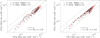 |
Fig. 6 Systematic comparison between the rate coefficients red(in cubic centimeters per second) of the CS–H2O system (x-axis) with the CO–H2O system (y-axis), with p-H2O in the left panel and o-H2O in the right panel) at 50 K (red crosses) and 100 K (black circles). |
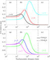 |
Fig. 7 Population of CS energy levels (2 ≤ jCS ≤ 7) as a function of the nucleocentric distance (in kilometers) using CS–H2O thermalized rate coefficients computed in this work (solid lines) and CO–H2O thermalized rate coefficients computed by Loreau et al. (2018a) and Faure et al. (2020, dashed lines) at 100 K. The range of nucleocentric delimits the following zones: (a) inner-coma, LTE; (b) mid-coma non-LTE; (c) outer coma fluorescence. |
5 Conclusions
In this work, we have studied the collisional excitation of CS induced by both p-H2O and o-H2O in the 5–100 K temperature range, relevant for the study of cometary comae. The study began with the determination of the PES characterizing the electronic interaction between the two colliders. This PES was computed using the SAPT(DFT) and aVQZ level of theory. The PES was found to be highly anisotropic and presents a deep global minima at approximately 1220 cm−1. The resulting 5D PES was implemented in the hibridon software to compute the adiabatic states of the collisional system. A probability was assigned to each adiabatic state following the SACM approach to compute the CS–p-H2O and CS–o-H2O state-to-state cross sections.
State-to-state rate coefficients were derived for transitions involving the first 19 rotational levels of CS (0 < jCS < 18), the first five levels of p-H2O (000 < jkakc < 220), and the first five levels of o-H2O (101 < jkakc < 303), over the 5–100 K temperature range. The accuracy of the rate coefficients was discussed, and they are estimated to be accurate at better than a factor of 1.5 based on the validation of CO–H2O data by Loreau et al. (2018a). Thermalized rate coefficients were calculated and used in non-LTE models to investigate the evolution of CS populations as a function of the nucleocentric distance. It was found that CS excitation is subject to strong non-LTE effects in the mid-coma, where excitation induced by solar radiation competes with collisional excitation induced by water molecules.
In addition, strategies for addressing the lack of rate coefficients in cometary atmospheres were examined. This study demonstrates that CS–H2 rate coefficients are not reliable substitutes for CS–H2O ones, nor is the global cross section suggested by Biver et al. (1999) a suitable alternative. Using CO–H2O rate coefficients was found to be the best alternative. This suggests that selecting rate coefficients involving H2O as the collisional partner and a chemically similar target molecule may yield more accurate modeling of the molecular excitation conditions than using data with the correct target molecule but with H2 as the collisional partner. Further studies on other cometary systems are needed to confirm this finding, although such analyses are currently hindered by the limited availability of relevant data for cometary applications.
Data availability
The state-to-state rate coefficients produced in this work will be available on the BASECOL database [https://basecol.vamdc.eu, Dubernet et al. (2024)], and thermalized rate coefficients will be available on the LAMDA [https://home.strw.leidenuniv.nl/~moldata/, Schöier et al. (2005)] and EMAA [https://emaa.osug.fr, Faure et al. (2025)] databases.
Acknowledgements
AGP and FL thanks financial support from the European Research Council (Consolidator Grant COLLEXISM, Grant Agreement No. 811363), Rennes Metropole, and the PNP program (INSU CNRS). JK thanks for the financial support from the US National Science Foundation subaward No. 362627Sub1 of Grant No. AST-2009253. JK also is greatful for computational time provided on University of Maryland High-Performance Computing clusters. DK would like to thank the COST Action CA21101 “Confined Electronic Systems” (COSY) and gratefully acknowledges support from the National Science Centre (NCN) under Sonata Bis 9 grant No. 2019/34/E/ST4/00407. FL thanks the Institut Universitaire de France. The scattering calculations were performed with GENCI (project No. A0170413001), and the cluster of the Institut de Physique de Rennes (IPR).
References
- Alexander, M., Dagdigian, P., Werner, H.-J., et al. 2023, Comput. Phys. Commun., 289, 108761 [Google Scholar]
- Biver, N., Bockelée-Morvan, D., Crovisier, J., et al. 1999, AJ, 118, 1850 [NASA ADS] [CrossRef] [Google Scholar]
- Biver, N., Russo, N. D., Opitom, C., & Rubin, M. 2022, arXiv e-prints [arXiv:2207.04800] [Google Scholar]
- Biver, N., Bockelée-Morvan, D., Crovisier, J., et al. 2023, A&A, 672, A170 [NASA ADS] [CrossRef] [EDP Sciences] [Google Scholar]
- Biver, N., Bockelée-Morvan, D., Handzlik, B., et al. 2024, A&A, 690, A271 [NASA ADS] [CrossRef] [EDP Sciences] [Google Scholar]
- Bockelée-Morvan, D. 1987, A&A, 181, 169 [Google Scholar]
- Bockelée-Morvan, D., Biver, N., Crovisier, J., et al. 2014, A&A, 562, A5 [NASA ADS] [CrossRef] [EDP Sciences] [Google Scholar]
- Bodewits, D., Bonev, B. P., Cordiner, M. A., & Villanueva, G. L. 2022, Radiative Processes as Diagnostics of Cometary Atmospheres (University of Arizona Press) [Google Scholar]
- Bustreel, R., Demuynck-Marliere, C., Destombes, J., & Journel, G. 1979, Chem. Phys. Lett., 67, 178 [Google Scholar]
- Calmonte, U., Altwegg, K., Balsiger, H., et al. 2016, MNRAS, 462, S253 [NASA ADS] [CrossRef] [Google Scholar]
- Cernicharo, J., Cabezas, C., Agúndez, M., et al. 2024, A&A, 688, L13 [NASA ADS] [CrossRef] [EDP Sciences] [Google Scholar]
- Cordiner, M. A., Coulson, I. M., Garcia-Berrios, E., et al. 2022, ApJ, 929, 38 [CrossRef] [Google Scholar]
- Cordiner, M. A., Roth, N. X., Milam, S. N., et al. 2023, ApJ, 953, 59 [Google Scholar]
- Crovisier, J. 1987, A&AS, 68, 223 [NASA ADS] [Google Scholar]
- Dagdigian, P. J. 2020, JCP, 152, 074307 [Google Scholar]
- Denis-Alpizar, O., Stoecklin, T., Guilloteau, S., & Dutrey, A. 2018, MNRAS, 478, 1811 [Google Scholar]
- Despois, D., Biver, N., Bockelée-Morvan, D., & Crovisier, J. 2006, IAU Proc., 1, 469 [Google Scholar]
- Dubernet, M. L., Boursier, C., Denis-Alpizar, O., et al. 2024, A&A, 683, A40 [NASA ADS] [CrossRef] [EDP Sciences] [Google Scholar]
- Endres, C. P., Schlemmer, S., Schilke, P., Stutzki, J., & Müller, H. S. 2016, J. Mol. Spectrosc., 327, 95 [NASA ADS] [CrossRef] [Google Scholar]
- Faure, A., Lique, F., & Remijan, A. J. 2018, JPCL, 9, 3199 [Google Scholar]
- Faure, A., Lique, F., & Loreau, J. 2020, MNRAS, 493, 776 [NASA ADS] [CrossRef] [Google Scholar]
- Faure, A., Bacmann, A., & Jacquot, R. 2025, A&A, 700, A266 [NASA ADS] [CrossRef] [EDP Sciences] [Google Scholar]
- Godard Palluet, A., Dawes, R., Quintas-Sánchez, E., Batista-Planas, A., & Lique, F. 2025, JCP, 162, 241101 [Google Scholar]
- Haser, L. 1957, Bull. Classe Sci., 43, 740 [Google Scholar]
- Herzberg, G. 1966, Molecular Spectra and Molecular Structure, 3: Electronic Spectra and Electronic Structure of Polyatomic Molecules (New York: van Nostrand Reinhold Comp) [Google Scholar]
- Joy, C., Mandal, B., Bostan, D., Dubernet, M.-L., & Babikov, D. 2024, Faraday Discuss., 225 [Google Scholar]
- Kalugina, Y. N., Faure, A., Van Der Avoird, A., Walker, K., & Lique, F. 2018, PCCP, 20, 5469 [Google Scholar]
- Loreau, J., Faure, A., & Lique, F. 2018a, JCP, 148, 244308 [Google Scholar]
- Loreau, J., Lique, F., & Faure, A. 2018b, ApJ, 853, L5 [NASA ADS] [CrossRef] [Google Scholar]
- Loreau, J., Kalugina, Y. N., Faure, A., Van Der Avoird, A., & Lique, F. 2020, JCP, 153, 214301 [Google Scholar]
- Loreau, J., Faure, A., & Lique, F. 2022, MNRAS, 516, 5964 [NASA ADS] [CrossRef] [Google Scholar]
- Lupu, R. E., Feldman, P. D., Weaver, H. A., & Tozzi, G.-P. 2007, ApJ, 670, 1473 [NASA ADS] [CrossRef] [Google Scholar]
- Mandal, B., & Babikov, D. 2023a, A&A, 678, A51 [NASA ADS] [CrossRef] [EDP Sciences] [Google Scholar]
- Mandal, B., & Babikov, D. 2023b, A&A, 671, A51 [NASA ADS] [CrossRef] [EDP Sciences] [Google Scholar]
- Mandal, B., Bostan, D., Joy, C., & Babikov, D. 2024, Comput. Phys. Commun., 294, 108938 [NASA ADS] [CrossRef] [Google Scholar]
- Metz, M. P., Piszczatowski, K., & Szalewicz, K. 2016, J. Chem. Theory Comput., 12, 5895 [Google Scholar]
- Misquitta, A. J., & Szalewicz, K. 2005, JCP, 122, 214109 [Google Scholar]
- Misquitta, A. J., Podeszwa, R., Jeziorski, B., & Szalewicz, K. 2005, JCP, 123, 214103 [Google Scholar]
- Müller, H. S. P., Thorwirth, S., Roth, D. A., & Winnewisser, G. 2001, A&A, 370, L49 [Google Scholar]
- Müller, H. S., Schlöder, F., Stutzki, J., & Winnewisser, G. 2005, J. Mol. Struct., 742, 215 [Google Scholar]
- Mumma, M. J., & Charnley, S. B. 2011, ARAA, 49, 471 [Google Scholar]
- Murphy, J. S., & Boggs, J. E. 1969, JCP, 51, 3891 [Google Scholar]
- Patkowski, K., Szalewicz, K., & Jeziorski, B. 2006, JCP, 125, 154107 [Google Scholar]
- Quack, M., & Troe, J. 1974, Ber. Bunsenges. Phys. Chem., 78, 240 [Google Scholar]
- Quack, M., & Troe, J. 1975, Ber. Bunsenges. Phys. Chem., 79, 170 [Google Scholar]
- Roth, N. X., Milam, S. N., Cordiner, M. A., et al. 2021a, ApJ, 921, 14 [NASA ADS] [CrossRef] [Google Scholar]
- Roth, N. X., Milam, S. N., Cordiner, M. A., et al. 2021b, PSJ, 2, 55 [Google Scholar]
- Schöier, F. L., van der Tak, F. F. S., van Dishoeck, E. F., & Black, J. H. 2005, A&A, 432, 369 [Google Scholar]
- Semenov, A., & Babikov, D. 2013, JCP, 138, 164110 [Google Scholar]
- Tonolo, F., Quintas-Sánchez, E., Batista-Planas, A., Dawes, R., & Lique, F. 2025, JCPA, 129, 9583 [Google Scholar]
- van der Tak, F. F. S., Black, J. H., Schöier, F. L., Jansen, D. J., & van Dishoeck, E. F. 2007, A&A, 468, 627 [NASA ADS] [CrossRef] [EDP Sciences] [Google Scholar]
- Zakharov, V., Bockelée-Morvan, D., Biver, N., Crovisier, J., & Lecacheux, A. 2007, A&A, 473, 303 [NASA ADS] [CrossRef] [EDP Sciences] [Google Scholar]
- Żółtowski, M., Loreau, J., & Lique, F. 2022, PCCP, 24, 11910 [Google Scholar]
- Żółtowski, M., Lique, F., Żuchowski, P., et al. 2025, MNRAS, 540, 626 [Google Scholar]
A channel represents a quantum state of the molecular system described by the quantum numbers {jCS, j, ka, kc, j12, l}, where jCS and j are the rotational quantum numbers of CS and H2O, respectively, ka and kc are the projections of j along the a, c inertia axis of the asymmetric top, j12 is the sum to the rotational angular momentum of each monomer and can take any integer value between |jCS − j| and jCS + j, and l is the relative angular momentum of the monomers that describes the relative rotation of the two monomers.
Originally, the EMAX option applies only to the linear monomer, so it was modified to apply to any channel.
The calculations were performed for several column densities, and the population of CS energy levels were not found to be very sensitive to this value. Therefore, this assumption is not expected to impact the following discussion.
As the CO–H2O has a well depth shallower than the CS–H2O, and CO has a rotational constant twice lower than CS, the convergence of CC calculations for the CO–H2O is achievable with a smaller rotational basis than what would be required for the present system. Thus, Loreau et al. (2018a) were able to converge a CC cross sections for a few lowest partial waves.
Collisional excitation induced by CO could also be considered to supplement for collisional excitation induced by H2O but only three sets of data currently exist with CO as a projectile: CO–CO (Żółtowski et al. 2022), CS–CO (Godard Palluet et al. 2025), and HCN–CO (Tonolo et al. 2025). Therefore, substituting the H2O by the CO collider does not appear as an efficient strategy, and it is not discussed here.
Appendix A Computational details about the SACM method
In the SACM method, the rotational basis for the adiabatic states calculations should include all rotational levels of both monomers that are energetically accessible up to the maximum total energy considered for the collision. In our case, the goal was to compute rate coefficients between all jCS ≤ 18 levels (at approximately 280 cm−1), and all jkakc ≤ 220 for p-H2O, and up to jkakc ≤ 303 for o-H2O levels (both are lying at approximately 137 cm−1). If we consider the kinetic energy distribution at 100 K to be of 400 cm−1, then the highest total energy of the collision is the sum of these energies, so around 817 cm−1.
According to the SACM method, any channels with an energy lower than this energy can be considered open, and have a non-zero probability in the adiabatic states counting. Therefore, any rotational level of both CS and H2O with an energy lower than 817 cm−1 should be included in the basis. Therefore, the ideal rotational basis would include all jCS ≤ 36, and all jkakc ≤ 10kakc for both p-H2O and o-H2O. Note that the conversion between p- and o-H2O being forbidden, the two sets of rate coefficients CS–p-H2O and CS–o-H2O are determined independently. However, employing this basis led to more than 10 000 channels for the partial wave J = 1, even with the EMAX option applied—surpassing the numerical limits typically acceptable for this type of scattering calculation. Consequently, truncation of the rotational basis was necessary.
The objective is therefore to reduce the size of the rotational basis without compromising the accuracy of the collisional rate coefficients obtained using the SACM approach. The truncated basis was finally set at jCS ≤ 31, jkakc ≤ 3kakc for CS-p-H2O, and jCS ≤ 26, jkakc ≤ 3kakc for CS-o-H2O. To ensure that this truncation was not affecting the quality of the data, the rate coefficients were computed with both rotational basis (full and truncated) for two partial wave as possible (J = 0, 1), and the two sets of rate coefficients are compared in Fig. A.1.
The WMEF was calculated based on Eq. (10), with ![Mathematical equation: $\[k_{i}^{\text {REF}} \equiv k_{i}^{\text {full}}\]$](/articles/aa/full_html/2026/03/aa57530-25/aa57530-25-eq27.png) , the rate coefficients computed based on the adiabatic states computed with the full rotational basis, and
, the rate coefficients computed based on the adiabatic states computed with the full rotational basis, and ![Mathematical equation: $\[k_{i} \equiv k_{i}^{\text {trunc.}}\]$](/articles/aa/full_html/2026/03/aa57530-25/aa57530-25-eq28.png) , the rate coefficients computed with the truncated rotational basis.
, the rate coefficients computed with the truncated rotational basis.
In this figure, we observe no significant differences between the two datasets, with a WMEF very close to unity in both cases. All dominant transitions are nearly perfectly reproduced by the truncated rotational basis, and the deviation remains within a factor of two at all times for the CS–o-H2O rate coefficients. Only a few of the weakest transitions exceed a factor of two for CS–p-H2O rate coefficients. Therefore, we conclude that this rotational basis can be reliably used to compute the CS–H2O collisional data within the SACM approach.
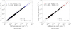 |
Fig. A.1 Comparison of the (a) CS-p-H2O (b) CS-o-H2O rate coefficients (in cm3 s−1) computed with the full (on the x-axis) and truncated (on the y-axis) rotational basis for the adiabatic states calculations at 50 K (red and blue crosses) and 100 K (black circles). |
Appendix B Comparison of CS–p-H2O and CS–o-H2O thermalized rate coefficients
Figure B.1 presents a systematic comparison between the CS–p-H2O and CS–o-H2O thermalized rate coefficients at 10 K and 100 K. The WMEF was calculated based on Eq. (10), with ![Mathematical equation: $\[k_{i}^{\mathrm{REF}} \equiv k_{i}^{\mathrm{CS}-p-\mathrm{H}_{2} \mathrm{O}}\]$](/articles/aa/full_html/2026/03/aa57530-25/aa57530-25-eq29.png) , the CS–p-H2O rate coefficients, and
, the CS–p-H2O rate coefficients, and ![Mathematical equation: $\[k_{i} \equiv k_{i}^{\mathrm{CS}-o-\mathrm{H}_{2} \mathrm{O}}\]$](/articles/aa/full_html/2026/03/aa57530-25/aa57530-25-eq30.png) , the CS–o-H2O rate coefficients.
, the CS–o-H2O rate coefficients.
It can be observed that both sets are relatively similar, with agreement always better than a factor of two at 100 K, and with nearly all transitions agreeing within a factor of two at 10 K. The WMEF values—1.36 at 10 K and 1.09 at 100 K—indicate that the dominant transitions are similar in both cases. The agreement between the o- and p-H2O rate coefficients improves as the temperature increases, which can be attributed to a reduced impact of the energy threshold as the temperature increases. This effect has also been observed and discussed by Żółtowski et al. (2025).
With regard to the similarities between the two datasets, it is unlikely that the ortho-to-para ratio chosen in the non-LTE modeling will significantly impact the modeling of CS in water-dominated comets.
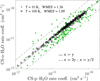 |
Fig. B.1 Systematic comparison between thermalized de-excitation rate coefficients of CS–p-H2O and CS–o-H2O collisional system at 10 K (green crosses) and 100 K (black circles). |
Appendix C Comparison of CS-H2O and CS-H2 rate coefficients
For the modeling of CS in water-dominated comets, the collisional rate coefficients of CS with H2O—previously unavailable—have sometimes been substituted with the CS–H2 rate coefficients computed by Denis-Alpizar et al. (2018) using the CC approach. To assess the accuracy of this approximation, the CS–H2O rate coefficients computed in this work are compared to the CS–H2 rate coefficients taken from the EMAA database (Faure et al. 2025) in Fig. C.1.
The deviations observed between the two sets of rate coefficients—those involving H2O and H2 as projectiles—are very significant. The dominant transitions tend to be stronger for CS–H2 compared to CS–H2O for both ortho- and para-H2O, whereas the weaker transitions are generally much stronger for CS-H2O thermalized rate coefficients. This is consistent with the behavior of rate coefficients involving light projectiles such as H2, which tend to decrease rapidly with increasing ΔjCS, while remaining relatively stable for heavier colliders like o/p-H2O.
The PES of the two collisional systems differ significantly in their well depths—the well for the CS–H2O system is much deeper than that for CS–H2 (1269 cm−1 vs. 173 cm−1). Since the intermediate complex formed by CS and H2O has a longer lifetime than the one formed with H2, the efficiency of the collision becomes less sensitive to the amount of energy transferred, and therefore less dependent on ΔjCS.
At 20 K, the global deviation, as indicated by the WMEF, is about 13.7 for p-H2O vs. p-H2 and 8.07 for o-H2O vs. o-H2. These deviations decrease to approximately a factor of 4 for both o/p-H2O vs. o/p-H2 at 100 K. This improvement can be attributed to the fact that, at higher temperatures, the rate coefficients involving H2 as a projectile tend to vary less with quantum numbers, thus aligning more closely with the behavior of the CS–H2O rate coefficients and reducing the overall deviation.
However, it is clear that the CS–H2 rate coefficients are not a reliable substitute for the CS–H2O rate coefficients. Using them in place of the appropriate data is likely to introduce significant inaccuracies in the derived physical conditions when modeling CS emission spectra in cometary comae.
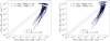 |
Fig. C.1 Systematic comparison between the rate coefficients (in cm3 s−1) of CS in collision with H2O (x axes) and H2 (y-axis) (p–H2/p–H2O in the left panel and o–H2/o–H2O in the right panel) at 20 K (blue crosses) and 100 K (black circles). |
Appendix D Comparison of CS-H2O and B99 rate coefficients
The global cross-section approach has been proposed by Bockelée-Morvan (1987) and Crovisier (1987), who derived the rate coefficients from a single global cross section adapted from the H2O-H2O pressure broadening experiment of Murphy & Boggs (1969). For CS–H2O rate coefficients, Biver et al. (1999) using a global cross section of σc = 5 × 10⁻¹⁴, cm2, from which they obtained B99 rate coefficients as ![Mathematical equation: $\[k_{c}(T)=\sigma_{c}~\langle v(T)\rangle n_{j_{\mathrm{CS}}^{\prime}}(T)\]$](/articles/aa/full_html/2026/03/aa57530-25/aa57530-25-eq31.png) , with ⟨v(T)⟩ being the mean velocity at the kinetic temperature T of the medium, and
, with ⟨v(T)⟩ being the mean velocity at the kinetic temperature T of the medium, and ![Mathematical equation: $\[n_{j_{\mathrm{CS}}^{\prime}}(T)\]$](/articles/aa/full_html/2026/03/aa57530-25/aa57530-25-eq32.png) being the population of the final CS level, assuming a Boltzmann distribution. In their approach, they do not differentiate between ortho and para water, and the rate coefficients inferred from this approximation are independent of the initial level.
being the population of the final CS level, assuming a Boltzmann distribution. In their approach, they do not differentiate between ortho and para water, and the rate coefficients inferred from this approximation are independent of the initial level.
The B99 rate coefficients are compared to the thermalized CS–H2O rate coefficients obtained in this work in Fig. D.1.
The deviation between the two sets of rate coefficients are particularly large, especially at 20 K where the WMEF indicate over two order of magnitude between the sets of data. This is due to the thermal weight attributed, which is going to be very low for certain CS level at 20 K, but remain relatively equally spread among CS energy levels at 100 K, thus leading to a better agreement with CS–H2O data.
It is important to note that B99 rate coefficients are systematically higher than the CS–H2O rate coefficients, suggesting an overestimation of the global cross section proposed by Biver et al. (1999). Such differences are still very significant, with a WMEF equal to 4.21, suggesting that this approximation is not expected to perform well to accurately constrain physical parameters from CS molecular spectra in comets.
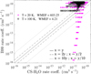 |
Fig. D.1 Systematic comparison between rate coefficients (in cm3 s−1) of CS in collision with thermalized H2O (x axes) and B99 rate coefficients (y-axis) at 20 K (magenta crosses) and 100 K (black circles). |
All Figures
|
Fig. 1 Comparison of the CS–H2O SAPT(DFT) and aVQZ PES fit (solid black line) with the CCSD(T)-F12 and aVTZ+BF calculations performed for selected radial cuts. The θ1 and ϕ1 are spherical angles of the R vector, while θ2 and ϕ2 are spherical angles describing the orientation of the CS molecule. |
| In the text | |
|
Fig. 2 Global minimum equilibrium geometry of the CS–H2O SAPT(DFT) and aVQZ PES. The Re between the c.o.m. of H2O and c.o.m. of CS is 8.11a0, with θ1 = 122°, θ2 = 297°, and ϕ1 = ϕ2 = 0°. |
| In the text | |
|
Fig. 3 SAPT(DFT) PES of the CS–H2O complex for varying orientation angles, θ1 and θ2, with ϕ1 = ϕ2 = 0° at R = 8.11a0. |
| In the text | |
|
Fig. 4 Representation of de-excitation thermalized rate coefficients (in cm3 s−1) of the CS–p-H2O (solid lines) and CS–o-H2O (dashed lines) from the first rotationally excited states (j1 = 1, 2, 3, 4) to the ground rotational state (j = 0). |
| In the text | |
|
Fig. 5 Population of CS energy levels (2 ≤ jCS ≤ 7) as a function of the nucleocentric distance (in km) using CS–H2O thermalized rate coefficients computed in this work (solid lines) and CS–H2 thermalized rate coefficients (dash-dotted lines) at 100 K. The range of nucleocentric delimits the following zones: (a) inner-coma, LTE; (b) mid-coma non-LTE; (c) outer coma fluorescence. Odd and even jCS have been separated for the sake of clarity. |
| In the text | |
|
Fig. 6 Systematic comparison between the rate coefficients red(in cubic centimeters per second) of the CS–H2O system (x-axis) with the CO–H2O system (y-axis), with p-H2O in the left panel and o-H2O in the right panel) at 50 K (red crosses) and 100 K (black circles). |
| In the text | |
|
Fig. 7 Population of CS energy levels (2 ≤ jCS ≤ 7) as a function of the nucleocentric distance (in kilometers) using CS–H2O thermalized rate coefficients computed in this work (solid lines) and CO–H2O thermalized rate coefficients computed by Loreau et al. (2018a) and Faure et al. (2020, dashed lines) at 100 K. The range of nucleocentric delimits the following zones: (a) inner-coma, LTE; (b) mid-coma non-LTE; (c) outer coma fluorescence. |
| In the text | |
|
Fig. A.1 Comparison of the (a) CS-p-H2O (b) CS-o-H2O rate coefficients (in cm3 s−1) computed with the full (on the x-axis) and truncated (on the y-axis) rotational basis for the adiabatic states calculations at 50 K (red and blue crosses) and 100 K (black circles). |
| In the text | |
|
Fig. B.1 Systematic comparison between thermalized de-excitation rate coefficients of CS–p-H2O and CS–o-H2O collisional system at 10 K (green crosses) and 100 K (black circles). |
| In the text | |
|
Fig. C.1 Systematic comparison between the rate coefficients (in cm3 s−1) of CS in collision with H2O (x axes) and H2 (y-axis) (p–H2/p–H2O in the left panel and o–H2/o–H2O in the right panel) at 20 K (blue crosses) and 100 K (black circles). |
| In the text | |
|
Fig. D.1 Systematic comparison between rate coefficients (in cm3 s−1) of CS in collision with thermalized H2O (x axes) and B99 rate coefficients (y-axis) at 20 K (magenta crosses) and 100 K (black circles). |
| In the text | |
Current usage metrics show cumulative count of Article Views (full-text article views including HTML views, PDF and ePub downloads, according to the available data) and Abstracts Views on Vision4Press platform.
Data correspond to usage on the plateform after 2015. The current usage metrics is available 48-96 hours after online publication and is updated daily on week days.
Initial download of the metrics may take a while.