| Issue |
A&A
Volume 707, March 2026
|
|
|---|---|---|
| Article Number | A107 | |
| Number of page(s) | 13 | |
| Section | Extragalactic astronomy | |
| DOI | https://doi.org/10.1051/0004-6361/202557543 | |
| Published online | 02 March 2026 | |
Ultra-diffuse galaxies in clusters: The peculiar gas loss of VCC 1964
1
Astronomical Institute of the Czech Academy of Sciences Prague, Czech Republic
2
Astronomical Institute of Charles University Prague, Czech Republic
3
National Radio Astronomy Observatory Socorro New Mexico, USA
★ Corresponding author.
Received:
3
October
2025
Accepted:
8
January
2026
Abstract
Context. Ultra-diffuse galaxies are low surface brightness systems that have been detected in H I in the field, where their line widths sometimes indicate significant dark matter deficits. They are rarely detected in H I in clusters, which makes their dynamical properties difficult to assess. The relation between field and cluster populations is unclear.
Aims. Detecting UDGs entering a cluster could give important clues about their evolution in terms of their dynamics, but also as to whether they are structurally similar, that is, if cluster UDGs are generally the same as field UDGs, but with less gas and an older stellar population.
Methods. We used data from two deep Arecibo surveys, the Arecibo Galaxy Environment Survey and the Widefield Arecibo Virgo Environment Survey, to measure the gas content of the UDG-candidate VCC 1964. The optical properties were quantified from the Sloan Digital Sky Survey and DESI Legacy Surveys.
Results. We found a significant 9 kpc offset between the H I and optical components of VCC 1964, no evidence of asymmetry in the H I, and only a modest deficiency level. This suggests a wholesale displacement of the gas content. The line width deviates by 4–5σ from the baryonic form and deviates by over 6σ from the optical form of the Tully-Fisher relation. The optical component is blue and smooth.
Conclusions. VCC 1964 is consistent with a UDG in which gas is displaced by ram pressure as it enters the cluster for the first time. Intriguingly, its dynamics imply a significant dark matter deficit, but we cannot rule out that the reason might be that its gas is displaced out of equilibrium.
Key words: galaxies: evolution / galaxies: general / galaxies: kinematics and dynamics
© The Authors 2026
 Open Access article, published by EDP Sciences, under the terms of the Creative Commons Attribution License (https://creativecommons.org/licenses/by/4.0), which permits unrestricted use, distribution, and reproduction in any medium, provided the original work is properly cited.
This article is published in open access under the Subscribe to Open model. This email address is being protected from spambots. You need JavaScript enabled to view it. to support open access publication.
1. Introduction
Ultra-diffuse galaxies (UDGs) are typically defined as being of low surface brightness (fainter than 24 mag arcsec−2) and having a large radius (Re ≥ 1.5 kpc). While their existence has been known for several decades (see Conselice 2018 for a brief review), only with the discoveries of van Dokkum et al. (2015) and Koda et al. (2015) has it become apparent that these are a distinct sub-class of low surface brightness (LSB) galaxies that are present in large numbers in clusters, but are also now known in groups (Román & Trujillo 2017) and in isolation (Leisman et al. 2017). They have diverse properties, with cluster UDGs typically being red and gas poor compared to those in lower-density environments, and consequently multiple pathways for their formation have been suggested (e.g. Buzzo et al. 2025). The dynamics of UDGs are particularly intriguing, with observations suggesting that some at least have little or no dark matter (van Dokkum et al. 2018, 2019). While this is still contested, resolved H I gas kinematics have supported this for UDGs that were found in isolation (e.g. Leisman et al. 2017; Mancera Piña et al. 2019, 2020). Although it has been argued that the low rotation velocities that suggest a lack of dark matter are due to errors in estimating the inclination angle (Oman et al. 2016) or other issues of data quality (Jones et al. 2023), stellar velocity dispersion measurements have confirmed low rotation speeds in at least some objects (Shen et al. 2023), and statistical studies show that the inclination measurements do not suffer from observational bias (Hu et al. 2023).
It is thus important to understand the relation between cluster and field UDGs to establish their more general significance. Importantly, the lower dark matter content has been suggested to result from galaxy-galaxy interactions (e.g. Silk 2019, Moreno et al. 2022), but this scenario has obvious problems for isolated UDGs. If these objects inherently lack dark matter and evolve into cluster UDGs only through gas loss and quenching of star formation (i.e. without any environmental processes that deplete their dark matter content), then this indicates the existence of a large number of galaxies with a reduced dark matter content. This poses challenges for cosmological models. Conversely, if field and cluster UDGs are formed by different mechanisms, then the field UDGs without dark matter might represent a rarer, more exotic class of objects. If a UDG were found to enter a cluster for the first time, with its gas content not significantly depleted by ram pressure, this could give important clues about the nature of the objects more generally.
Relatively small numbers of field UDGs are known in comparison to cluster members, but far more of the former have dynamical measurements from their gas content. This makes the connection between the two populations unclear. In addition to the dynamics, differences in globular cluster (GC) populations have also been noted. Jones et al. (2023) reported that gas-rich UDGs in the field tend to have very few GCs, whereas cluster members have rich GC populations. The authors therefore argued against the results of Junais et al. (2022), who found that ram-pressure stripping reproduces the colours and brightness profiles of cluster UDGs well if they resulted from an infalling field population. The situation is nuanced, however. Jones et al. (2023) noted that GCs in UDGs in other clusters differ, with Hydra UDGs having smaller populations, and they accepted that some small cluster UDGs might result from field infall (we also note that their study did not include Virgo, which was the focus of Junais et al. 2022). Forbes et al. (2020) reported evidence for a wide range of GCs within Coma UDGs, with most of their sample being GC-rich, but others having populations that are more consistent with dwarf galaxies. Finally, in Virgo, which we study here, the situation is unclear. Lim et al. (2020) found that Virgo UDGs have slightly fewer GCs than elsewhere, but the sample size of 26 is much smaller than in other clusters. The authors also noted that direct comparisons are complicated by the different luminosities and surface brightnesses of the samples.
The number of UDGs with H I detections (hereafter HUD, following Leisman et al. 2017) remains low, with Leisman et al. (2017) and Janowiecki et al. (2019) reporting a total of 252 HUDs; a few more were reported for example by Spekkens & Karunakaran (2018), Shi et al. (2017), Papastergis et al. (2017), and Karunakaran et al. (2020), with another 37 by Karunakaran et al. (2024). The number of HUDs known in rich clusters is considerably lower. Spekkens & Karunakaran (2018) identified a total of 5 HUDs in or near Hickson compact groups, while of the 252 ALFALFA-identified HUDs (Arecibo Legacy Fast ALFA, Giovanelli et al. 2005), Janowiecki et al. (2019) found only 10 within two virial radii of any group (with none identified as being in rich clusters). The latter authors concluded that gas-poor UDGs in clusters might result from the infall and stripping of HUDs, and their optically diffuse nature does not result from environmental effects. Sandoval Ascencio et al. (2025) recently discovered seven post-starburst UDGs, three of which are isolated, and four are satellites of massive systems. Presumably, these post-starburst objects are gas deficient, but the detection of a UDG actually caught in the process of losing its detected neutral gas has yet to be convincingly demonstrated.
One such candidate was proposed by Junais et al. (2021). They found a candidate UDG NGVS 3543 in the Virgo Cluster, just north of an apparent star-forming wake (with associated H I emission) catalogued as AGC 226178. The two objects were well aligned with the cluster centre, which is suggestive of ram pressure. This interpretation was challenged by Jones et al. (2022a), who reported that NGVS 3543 is more likely at a distance of only 10 Mpc, as is the nearby dwarf galaxy VCC 2037. They also discovered a long H I tail extending from both the UDG candidate and patchy stellar emission to the brighter (cluster member) galaxy VCC 2034. They therefore suggested that AGC 226178 is the result of star formation in this stripped gas. Subsequently, Junais et al. (2022) reported that their own modelling gave results that were consistent with the Jones et al. (2022a) scenario. Very recently, Sun et al. (2025) have questioned the existence of the long H I structure, which raises further doubts about the origin of AGC 226178.
The complex environment and distance uncertainties of NGVS 3543 make it difficult to assess as a candidate for a UDG experiencing ram pressure stripping. Determining the location and manner in which UDGs are quenched remains a matter of some difficulty. Grishin et al. (2021) suggested that UDGs in clusters originate from the gas loss and stellar expansion of relatively massive discs entering clusters on tangential orbits. In contrast, Benavides et al. (2021) suggested that currently isolated UDGs are backsplash galaxies that were quenched in clusters, but that UDGs were diffuse from their birth in high-spin dark matter haloes and not as a result of evolution within clusters. Sandoval Ascencio et al. (2025) found that at least some UDGs were quenched in the field and explicitly ruled out a backsplash origin because the objects are isolated and have a post-starburst nature, although this does not preclude quenching that also results from environmental effects. Finally, Hartke et al. (2025) presented the opposite possibility that some UDGs could be born in clusters from ram-pressure stripped material (see also Dey et al. 2025; we discuss this in more detail in Section 4).
Clearly, UDGs are difficult to assess as a population in general, and they almost certainly result from a multitude of different processes in different environments. In this context, we present a new candidate for a UDG that experiences gas loss in the Virgo cluster, VCC 1964. This object appears to reside in a far simpler local environment within the cluster than NGVS 3543. VCC 1964 was first claimed as an H I detection in data from the ALFALFA survey in di Serego Alighieri et al. (2007), but the authors regarded this as very tentative, and it was not included in the final ALFALFA data releases. In contrast, its detection in the deeper AGES survey (Arecibo Galaxy Environment Survey, see next section for details) was unambiguous and assigned the ID AGESVC1 275 in Taylor et al. (2012) (hereafter, AGES V). Its significance as a possible UDG was not noted until the SMUDGES project (Systematically Measuring Ultra Diffuse Galaxies; SMDG 1243207+085703 in Zaritsky et al. 2023), who did not identify the H I counterpart. We present the optical and H I data together. We show that VCC 1964 is a compelling candidate for a UDG in the process of losing gas through ram pressure as it enters the cluster. For consistency with previous AGES results, we adopt H0 = 71 km s−1 Mpc−1 and a Virgo cluster distance of 17 Mpc.
The remainder of this article is organised as follows. In Section 2 we describe the observational data we used in this analysis, particularly the Arecibo H I data. Section 3 describes the observational evidence for the two main distinguishing features of VCC 1964 : Its H I gas appears to be displaced from its stellar component, and it is significantly offset from the Tully-Fisher relation. We describe in detail how we obtained these results and how secure they are given the uncertainties in the data. Finally, we interpret these findings in Section 4.
2. Observations and data analysis
Our H I data come from AGES and its direct successor survey WAVES, the Widefield Arecibo Virgo Environment Survey. Both surveys used an identical observing setup, of which full descriptions can be found in Auld et al. (2006), Minchin et al. (2010), Davies et al. (2011), and Minchin et al. (2019). We only summarise the main parameters of the surveys here and refer readers to the earlier papers for full technical details.
2.1. Observing setup
In brief, AGES was a fully sampled drift-scan survey using the seven beam Arecibo L-band Feed Array instrument ALFA. Each beam records data from two orthogonal polarisations with the final reduced data being an average of the two. AGES mapped (among others) two regions of the Virgo cluster to an rms of 0.6 mJy at spatial and spectral resolutions of 3.5′ and 10 km s−1 (after Hanning smoothing – see below and also Section 3.4.1), respectively, with a 1 σ column density sensitivity of 1.5 × 1017 cm−2(Δ V / 10)1/2 (Keenan et al. 2016). The full bandwidth of AGES was equivalent to a velocity range of –2000 to +20 000 km s−1, but we here only used data pertaining to the Virgo cluster. The main results from Virgo are found in AGES V and also AGES VI (Taylor et al. 2013), but the latter covers as different area of the cluster and is not used in the present study.
AGES V presented the main AGES results in Virgo, a 10×2 degree field (R.A. versus Declination) centred on M49 deemed AGES VC1. This is a complex region with galaxies believed to be in the main body of the cluster (17 Mpc distance) but also in two infalling clouds at 23 and 32 Mpc. Distances were assigned based on the measurements and characterisations given in Gavazzi et al. (1999). As described in AGES V Section 4.2 (especially Figure 6; see also Taylor 2010 chapter 5, Section 5.3.2), the boundaries determined for these different groups are uncertain, and the original two-dimensional assignments from Gavazzi et al. (1999) are, in some cases, not-well matched with the velocity data. However, VCC 1964 is well inside the limits of the 17 Mpc main body of the cluster, being almost three degrees from the boundary. Additionally, as we discuss in Section 3.7, a greater distance would make VCC 1964 an even more extreme object than its data otherwise indicates. If VCC 1964 is a cluster member, this is little room for doubt regarding its distance, but as we shall show, there is somewhat more of a concern as to whether it really is within the Virgo cluster at all.
WAVES was intended as a successor to AGES that would eventually map the entirety of Virgo to the AGES depth and resolution. This was envisaged as a staged project, with the WAVES South data we use here being fully observed and a northern field still in progress at the time the telescope collapsed. As shown in Minchin et al. (2019), the WAVES South field fills in the area immediately north of the AGES VC1 field, having the same boundaries in R.A. and a small overlap in declination – exactly where VCC 1964 happens to be situated (AGES VC1 has a northern declination limit of +09°07′whereas the southern limit of WAVES South is +08°52′). Note that AGES and WAVES use completely different observations, thus they provide independent measurements of the same region in this case.
The hexagonal beam pattern of ALFA means that at the extreme spatial edges of the surveys, sensitivity is reduced as not all of ALFA’s seven beams sample the whole range of declination or R.A. While VCC 1964 is in the region of homogenous sensitivity in the AGES VC1 data, it is within the region of reduced sensitivity in the WAVES data. Despite this, WAVES provides two important contributions : (1) it verifies the H I parameters as measured in AGES; (2) it enables a search of a larger area for H I-detected galaxies that might be alternative progenitors of AGESVC1 275. Here we also combine the AGES and WAVES H I datasets, with the overlap region being an average value weighted by the rms levels. First results of the WAVES survey were presented in Minchin et al. (2019) while Partík et al. (in prep.) will present the full catalogue of the whole WAVES South region.
2.2. Data reduction and analysis
The data reduction for the two surveys was carried out using a combination of LIVEDATA, GRIDZILLA (Barnes et al. 2001) and our own post-processing techniques (Taylor et al. 2014); the important aspect of the latter here being the use of a second-order polynomial fit to each spectrum in the data. As standard, the data also has Hanning smoothing applied post-gridding, which removes the effect of Gibbs ringing and decreases the rms (see e.g. Barnes et al. 2001). The cost of this is a reduction in spectral resolution by a factor two, not normally a concern: the unsmoothed data has a channel width of 5 km s−1, so degrading this to 10 km s−1 does not usually have much impact since this is the approximate width of the H I line itself. The spatial pixels were set to 1′.
Source extraction techniques and efficacy are discussed in detail in Taylor (2025b). In brief, for the AGES and WAVES data, we used visual inspection using the FRELLED package, which was originally developed specifically for AGES data (Taylor 2015, 2025a). This follows our standard two-stage procedure. First, users inspect the data in a 3D volumetric display, interactively masking visible sources (identified through training, based on the known appearance of real extragalactic H I detections – see Taylor (2025b), in particular Section 4.4.1). A volumetric display is extremely convenient for showing the 3D structure of a source, making the masking process rapid and straightforward. The limitation of this is that, due to the necessity to restrict the display of the data to the brightest voxels in 3D (otherwise the display is overwhelmed by noise), only the relatively bright sources are clearly visible. The second stage proceeds with this masked data in 2D, displaying slices of the data (e.g. channel maps) as conventional images. Masking here is more laborious as the user must continually scroll through the images to check exactly where the source is visible, but has the advantage of not requiring any cuts in the data – thus ensuring that even the faintest sources are visible. Once catalogued, as with all AGES and WAVES analysis, we measure the H I parameters using the msbpect task from the MIRIAD package (Sault et al. 1995).
The efficacy of the source extraction procedure was quantified in Taylor (2025b). It was found that the completeness rate closely follows the integrated S/N as defined in Saintonge 2007 equation 16, which we give here in the slightly modified form used in most ALFALFA papers (e.g. Haynes et al. 2018),
 (1)
(1)
where for W50 < 400 km/s, wsmo = W50/(2 × vres), where vres is the velocity resolution in km/s, and for W50 > 400 km/s,  . Fc is the total flux in Jy km s−1; rms is the rms across the spectrum in mJy.
The completeness rate for visual source extraction of unresolved sources was shown to approach 100% when the S/Nint exceeds a critical threshold of 6.5. For VCC 1964 in the AGES data this was measured at 21.9 – well beyond the point where any follow-up was thought necessary, given that the unusual properties of the source we describe here were not identified during the initial discovery. In Section 3.3.2 we also present the results of searching the combined AGES and WAVES dataset using automated techniques. The data combination was performed with a custom Python script.
2.3. Optical data
In AGES V we relied on optical data from the SDSS and measurements given in the VCC and GOLDMine. Though its LSB-nature was not recognised in AGES V, it was noted as unusual due to its morphological assignment (obtained from the GOLDMiNe database of Gavazzi et al. 2003, itself derived from the Virgo Cluster Catalogue of Binggeli et al. 1985) as an early-type galaxy, but its blue colour in the SDSS data (g–i = 0.32) implied that this classification was erroneous (its position on the colour-magnitude diagram can be seen in AGES V Figure 14 as the red triangle in the lower right corner of both panels). Here we use the parameters as measured in SMUDGES, which is based on the more sensitive DESI Legacy Survey (LS) data (Dey et al. 2019), with sensitivity of 29 mag arcsec−2 (r band, Martínez-Delgado et al. 2023). We note that while there is some uncertainty regarding the exact values of the optical parameters (particularly derived quantities such as stellar mass), the qualitative nature of the object is clear: this is a blue, structurally smooth LSB galaxy. While its effective radius may be slightly below the putative 1.5 kpc value for UDG status, this does not affect its physical nature (that is, its properties may be quantitatively different but qualitatively – e.g. dark matter content – similar), as discussed in detail in Buzzo et al. (2025). We note also that alternative, more complex definitions of UDGs have been proposed, e.g. Lim et al. (2020), while Sandoval Ascencio et al. (2025) allow a more liberal definition of UDGs down to Re ≥ 1.0 kpc. For simplicity, we default to referring to VCC 1964 as a UDG or UDG-candidate throughout the remainder of this work, noting that it is unclear whether so-called ‘nearly UDGs’ are really a distinct class of object (Buzzo et al. 2025).
3. Results
There are two unusual aspects of VCC 1964 that we discuss in turn. First, there is a clear offset between the H I and optical components that is highly atypical, with the gas closer in projection to the local cluster centre than the stellar emission. Second, the object is a significant outlier on the Tully-Fisher relation (TFR; we prefix this with baryonic or optical as appropriate, but the results are the same), having a lower line width than expected given its baryonic mass or optical luminosity. Throughout this section we describe how we obtained these results and the scope for errors, allowing for possible effects of systematic uncertainties (which dominate over the formal imprecision of the measurements).
3.1. Measured parameters
Table 1 gives the object’s most significant parameters (observed and derived) as per our best estimates. For these we use the H I parameters as measured in the combined AGES and WAVES cubes; for the optical data a combination of the SDSS and results from SMUDGES. Specifically: the coordinates are those of the H I detection; the apparent magnitudes are from SDSS data using modified SMUDGES parameters; the absolute magnitudes are corrected from Galactic and internal extinction; the stellar mass uses the prescription of Durbala et al. (2020); the inclination angle and effective radius comes from SMUDGES; the rotation velocity accounts for inclination angle as well as correcting for the difference between the maximum versus flat part of the rotation curve.
Selected properties of VCC 1964 and its associated H I detection (see text for details).
We discuss all of these in detail in the remainder of this section. One simple parameter is the H I mass, obtained from the flux via the standard equation,
 (2)
(2)
where d is the distance in Mpc. We note that the H I mass is lower than all of the HUDs given in the Janowiecki et al. (2019) sample, but they impose a minimum distance of 25 Mpc; similarly only three objects in the Janowiecki et al. (2019) sample have a comparable or more positive (i.e. fainter) absolute g magnitude. To our knowledge, given the other HUD samples cited earlier, this gives VCC 1964 the lowest H I mass of any UDG detected to date. The measured W50 places it in the bottom 10% of the Janowiecki et al. (2019) sample. Colours are difficult to compare given the still limited and inhomogeneous data available for HUDS, but as described in Section 2.3, VCC 1964 is well within the blue cloud.
The baryonic mass is calculated as Mbar = Mgas + M*. We discuss the stellar mass separately below. The gas mass is calculated by a correction for helium simply as Mgas = 1.36 MH I. We neglect molecular gas as its contribution is likely to be small (e.g. Leroy et al. 2005, McGaugh (2012), Grossi et al. 2016, Kado-Fong et al. 2022) and would only exacerbate the deviation from the TFR.
3.2. Offset between the optical and H I components
Figure 1 shows the combined AGES and WAVES H I contours overlaid on an LS RGB image. Individually, the two H I datasets show the same offset between the H I fitted centroid and the optical coordinates of the galaxy, approximately 1′50″, 9 kpc in projection. This is a factor 5.5 greater than the AGES median H I-optical offset of 20″, and the similarity of the H I coordinates from two independent datasets strongly suggests that this is a real effect and not due to the effects of noise in fitting the position (with a peak S/N of 19.6 in AGES, noise is not likely to greatly affect the fitted coordinates). The position of the H I and optical counterpart do not well align with the direction to M87 (the nominal centre of the main body of the cluster), with the angular difference between the H I-optical and M87 directional vectors (measured from the optical centre) being 114°. In contrast the angular difference with the direction of M49 (the centre of the local subgroup) is only 49°. M87 is 4.63° away (1.37 Mpc in projection) from VCC 1964 while M49 has an angular separation of 3.46° (1.03 Mpc).
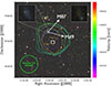 |
Fig. 1. Renzogram of 3.5σ H I contours of VCC 1964 from the combined AGES/WAVES datasets, overlaid on an LS RGB image. The white square and cross mark the positions of the H I centroid and optical position of the galaxy, respectively. The white arrows show the direction vectors to the giant ellipticals M87 and M49, the centre of the main body of the cluster, and the local sub-group. The whole image is 15′ across and ≈75 kpc at the assumed distance of 17 Mpc. The inset images show the same close-up field of view of VCC 1964, with the optical LS data on the left, and GALEX UV on the right. |
As described, we measure the H I parameters using the msbpect task from the MIRIAD package. This relies on user-input initial estimates for the spatial and spectral coordinates and the spectral profile range over which to integrate. Although mbspect then refines the parameters algorithmically, the subjective nature of the initial guesses cannot be fully removed. We therefore tried adjusting our original input parameters in each case, keeping them visibly consistent with the resultant spectra, and also comparing the fitted spatial position with the H I contours. Adjusting the input parameters and/or using a different dataset (AGES VC1, WAVES, or the combined cube) can give a fitted position as much as 22″ further south than the value reported in Table 1 (increasing the H I and optical offset), but a position 36″ further north is also compatible with the data (lessening the H I/optical offset). The value used here is the compromise case, which gives by far the best visual agreement with the H I contours. Thus we regard the reported offset as secure and not an artefact of data reduction or analysis method.
3.2.1. Ram pressure as a cause of the gas displacement
The offset of the H I and optical component is consistent with the H I either being stripped or displaced from (its presumed parent galaxy) VCC 1964 due to ram pressure, a natural explanation given the prevalence of such features in Virgo (Taylor et al. 2020) – provided, of course, that the object really is a cluster member, to which we return in Sections 3.5 and 3.7. We note also the presence of brighter blue feature at the south-west tip of the optical component, aligned with the gas displacement and also visible in GALEX data. Such a feature is qualitatively consistent with a galaxy experiencing the onset of ram pressure, which has been shown to trigger the formation of molecular gas and an increase in star formation activity (e.g. Jáchym et al. 2019, Cramer et al. 2020, Grishin et al. 2021).
Two caveats potentially complicate this interpretation. Firstly, the misalignment of the optical, H I, and direction vector to M49 of nearly 50° implies a rather non-radial orbit. This is not likely a significant problem. Observationally, we saw in Taylor et al. (2020) that other systems believed to be experiencing ram pressure also show tails collectively pointing away from the local centre but in imperfect alignments (see also Yagi et al. 2010, 2017 and Grishin et al. 2021, who interpret misaligned Hα tails in the same way). This is likely the result of several contributing factors: the cluster is non-spherical and has a complex structure, thus allowing for inherently non-radial orbits; harassment will distort ram pressure tails (in Taylor et al. 2017 we saw stripped tails of extreme morphological complexity resulting purely from the effects of tidal encounters); density variations within the ICM may cause non-radial tails.
Secondly, and more significantly, the H I is found closer to M49 than the optical component. Since the gas should trail the motion of the galaxy, this implies that either this is a backsplash galaxy (having already passed pericentre) or is on a strongly non-radial orbit.
The backsplash interpretation is in our view problematic. This would require a low-mass dwarf to have traversed at least a couple of megaparsecs through the cluster with only a modest gas loss (see Section 3.5.1) until the present moment, when the entirety of its remaining gas appears to have been displaced. We are not aware of any other backsplash candidates of masses this low that are still relatively gas rich; naively, we would expect a dwarf like this to have been almost completely stripped having crossed such a large swathe of the cluster. While Benavides et al. (2021) propose backsplash galaxies to explain isolated quiescent UDGs, their objects are red, spheroidal, and gas-poor (perhaps completely gas free, with the bulk of the gas loss occurring at pericentre passage). VCC 1964 is blue, disc-like, and if not obviously gas rich, then it still has gas in its immediate vicinity despite being long past pericentre.
We regard the scenario that the galaxy is on a non-radial orbit but just entering the cluster for the first time as a more promising alternative. This explains the abundance of gas, the alignment of the blue/UV feature with the displaced gas, and the one-sided displacement of the gas from the galaxy. A non-radial orbit would imply (by definition) a significant motion across the sky, which is consistent with the galaxy’s small difference in velocity (200 km s−1) compared to the cluster itself: if indeed the galaxy is losing gas through ram pressure, we would normally expect a much higher motion relative to the ICM than this.
3.2.2. Gas displacement from a tidal encounter
We have already suggested tidal encounters as possibly contributing to the angular misalignment of the gas and stellar components. It is also possible that the gas removal itself was largely the result of a tidal encounter rather than ram pressure. We note this as a valid alternative, but a less likely explanation for the gas displacement. VCC 1964 is in a relatively underdense region of the Virgo cluster, with the nearest H I detection 0.82 degrees away (AGESVC1 271, VCC 2033 – 240 kpc in projection). The nearest VCC galaxy (VCC 1980) is considerably closer at 13.2′ (65 kpc in projection), but this is an early-type galaxy and so unlikely to be the source of the gas. Of course, it could have instead only tidally disturbed VCC 1964 rather than providing its gas content (its systemic velocity is within 200 km s−1 of that of VCC 1964), but the lack of a counter-tail structure makes this less likely: contrary to the effects of ram pressure, we would not expect such a neat, one-sided displacement of the gas in that scenario but rather messier structures (e.g. Taylor et al. 2017; a major caveat here is, of course, the unresolved nature of the H I detection). Wholesale gas displacement as apparent here is not unknown in Virgo (e.g. VCC 1249 as discussed in AGES V) but is rare.
3.3. Is the gas really associated with VCC 1964?
One other possibility for explaining the misaligned gas and stars of VCC 1964 is that the gas is not really associated with the stellar component at all. The proximity of the H I and optical components seem too close to attribute to coincidence, but this has been strongly argued to be the case for the NGVS 3543 system; without an optical redshift we cannot entirely exclude this possibility. It is therefore worthwhile to undertake an additional search of the H I data, as this may reveal other potential sources of the gas.
Given that the H I detection associated with VCC 1964 is a bright source, if VCC 1964 were not itself the donor then we would expect the real source of the gas to be comparably bright. Per the completeness thresholds established in Taylor (2025b), the chance of missing such a source is negligible. However, the line width of VCC 1964 is very small, and if the parent galaxy had broader emission (as we might expect for more typical galaxies), it could be much fainter and more likely to have evaded detection. Additionally, there is the possibility of sources that are fainter than VCC 1964, which might give different clues to its origin: an alignment of such features might indicate the remains of a stream, or perhaps demonstrate that VCC 1964 is itself in the process of losing gas. Furthermore, the prospect of detecting faint sources in the AGES VC1 part of the combined AGES/WAVES dataset is relatively high, as this was not previously searched with our more recent source extraction techniques and software described below.
To conduct this search, we extracted a subset cube measuring 112′ on a side, about 550 kpc in projection, spanning the full velocity range of the cluster (0–3000 km s−1). This is large enough to include the three nearest H I detections known from our earlier examination. We performed both a visual search and used the automated source finder SoFiA-2 (Westmeier et al. 2021). The merits of each method are discussed in detail in Taylor (2025b), but the key point here is that SoFiA is easily able to apply multiple levels of spatial and spectral smoothing in order to search for emission that is extended on multiple scales. This is typically not done for visual searches owing to the time-consuming nature of the procedure, though in this case we also visually searched the cube after applying several different smoothing kernels.
3.3.1. Visual search
The visual search proceeded in the standard way, as described in Section 2.2. In brief, we visually scanned all R.A.-velocity slices of the cube, interactively masking any emission that resembles a real source (primarily by being sufficiently bright and coherent over several channels/slices). We then examined each candidate source by inspecting the spectra and constructing renzograms. These methods both helped by adding an additional check on whether the perceived signal arises from genuine, coherent emission in the data, or if it was only due to a chance alignment of pixels. We explored the use of renzograms in detail in Taylor et al. (2020), demonstrating that real signals typically correspond to coherent emission of two or three beams across (and/or the same number of channels) at a (peak) S/N threshold of 3.5 or greater. Finally, we also inspect optical data of the candidates from the SDSS and LS, as this can provide additional validation for faint sources.
The search was carried out with a conscious effort to be extremely liberal in designating candidate sources, provisionally accepting signals we would usually dismiss as they would be too weak to verify. 14 such candidates were found from a pure visual inspection of the cube. Our additional checks rejected nine of these due to weakness of the signal and incoherency of the spectrum and/or contours (i.e. having contours with different sizes and position from channel to channel), all of which also entirely lacked optical counterparts. The remaining five are marginal but cannot be immediately dismissed for our purposes here. In fact, one of these is a secure detection of the object designated as BC 13 in Dey et al. (2025), which we will describe in detail in a future publication. Stressing that we would ordinarily reject all of the remaining four candidates entirely, none appear to have any obvious relation to VCC 1964. Three are more than 800 km s−1 different in velocity, BC 13 itself is 28′ from VCC 1964, while the remaining object is nearly 1° away (300 kpc in projection).
3.3.2. Automatic search
For the SoFiA search, we use the parameters largely as determined in Taylor (2025b). As above, the chance of detecting even weak signals here is not high, especially given the finding that SoFiA tends to recover the same population of sources that can be found visually. Nevertheless, the overlap between the visual and automatic catalogues is not exact, and the capability of SoFiA to spatially smooth means that there is at least a chance it might detect a larger extended feature that is not visible in the standard cube.
The search parameters have been shown to closely reproduce, and even slightly exceed, the completeness level of a visual search for unresolved sources. Although this sacrifices reliability, the cube searched here is small, making it feasible to inspect each candidate for validation. We do this in the same way as described above: SoFiA candidates are imported as mask regions into our inspection software, which we then use for extracting spectra, generating renzograms, and querying the SDSS and LS (though due to the number of candidates we do not inspect every source by every method). The search parameters are This returned 113 candidate sources. Of these, apart from those found by other methods and searches in this same area, only two are at all plausible, having weak but clear signals in their spectra, coherent contours in the renzograms, and possible optical counterparts. Furthermore, as with the additional sources found visually, these are still very marginal detections that we would normally disregard from initial publication as they are impossible to confirm without additional observations (we are seeking follow-up for these and other sources in the WAVES area). Moreover, both are > 0.5° and > 1000 km s−1 from VCC 1964, making them very unlikely to have any association with our main target.
  scfind.kernelsXY = 0
  scfind.kernelsZ = 0, 3, 5, 7, 9, 11,
  13, 15, 17, 19, 21, 23, 25, 27, 29,
  31, 33, 35, 37, 39, 41
  scfind.threshold = 3.5
  linker.radiusXY = 2
  linker.radiusZ = 3
  linker.minSizeXY = 3
  linker.minSizeZ = 4
  reliability.enable = false
We also experimented with using different spatial smoothing kernels, which has the potential to reveal faint, extended structures (such as H I bridges and tails) that are below the nominal detection limits. A similar experiment was already performed in Taylor (2010) (see chapter 7, especially Sections 7.3.1 and 7.3.4), which smoothed over 800,000 areas of different sizes and shapes, but only using spatial smoothing. In that earlier study, no credible detections were found, with all candidates being of extremely narrow line width: to maintain a line width of a few km s−1 in a stream that is extended for tens of kiloparsecs is extremely unlikely, especially given that the line width of the parent galaxies is generally expected to be at least an order of magnitude greater.
For the SoFiA search we tried using spatial smoothing kernels of 9, 11, 13 and 15 pixels, corresponding to physical sizes of 45 to 75 kpc. All searches resulted in approximately 50 detections (tending to be the same structures in all cases), which have the appearance of randomly distributed ‘blobs’ of varying velocity widths, distributed throughout the search volume. Based on their position, orientation and morphology, none appear to have any relation to VCC 1964. As a control test we ran the same search on a subset of the Mock spectrometer data used in Taylor (2025b), where we are certain that no real emission is present due to its high blueshift. The subset was selected to have the same volume as the AGES VC1 area we inspect here. 83 sources were found, even more than in the AGES VC1 search area, demonstrating that the results are consistent with the effects of noise. Increasing the ‘scfind.threshold’ parameter does not really help, only reducing the number of detections and their sizes.
Based on this, we cautiously suggest that the smoothing used in SoFiA in Jones et al. (2022b) might be responsible for the claimed detection of a large H I stream in the NGVS 3543 system, which is not seen in either the WAVES or FAST data of similar sensitivity. Given the presence of two clear H I detections in this region, spatial smoothing might increase the apparent size of each source, and since these are relatively close, this may result in the appearance of a connecting bridge. A significant caveat is that the position-velocity diagram used in Jones et al. (2022b) is not a simple R.A-velocity slice. A more dedicated study is needed to confirm if the large ALFALFA stream is consistent with smoothing of the noise or if the detection does indeed result from a real, physical structure in the data.
In short, few new credible candidate sources were found, and none at all with any apparent relation to VCC 1964. By far the most likely source of the AGESVC1 275 gas cloud is VCC 1964 itself.
3.4. Deviation from the Tully-Fisher relation
The line width of the H I detection is among the lowest of the AGES sample with W50 = 26 km s−1; of the 1,231 published AGES sources only 18 (1.4%) have line widths equal or lower than this value – spectra are shown here in Figure 2. This gives the galaxy a 4.5 σ deviation from the Baryonic Tully-Fisher Relation (BTFR; McGaugh et al. 2000) as shown in Figure 3, increasing to 5.3σ if we use the unsmoothed AGES cube. This offset is robust to measurement errors in the optical photometry. To bring the galaxy within the 2σ scatter would require an inclination angle of 40°, which is grossly incompatible with the optical data (see Figure 4). Figure 3 also shows for comparison the galaxies of Mancera Piña et al. (2019). These are more than an order of magnitude more massive and generally of higher line width, yet show even stronger deviations. Note that we show these using the values given directly in Mancera Piña et al. (2019) (who use resolved H I maps for modelling the rotation curves), and given the numerous corrections we apply to our own data, the comparison should be taken too literally. We also caution that it is far from the case that every UDG shows similar deviations: indeed, some have been claimed to be overmassive rather than having a dark matter deficit (most famously Dragonfly 44, van Dokkum et al. 2016; Saifollahi et al. 2021, but see also e.g. Beasley et al. 2016, Forbes et al. 2020).
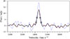 |
Fig. 2. H I spectra of VCC 1964 from AGES (blue), WAVES (red), and the combination (black). The circles and squares show the fitted W50 and W20 velocity widths, respectively. |
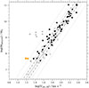 |
Fig. 3. Baryonic Tully-Fisher as in Taylor et al. (2022). The filled black circles use AGES H I data and SDSS photometry, from the H I detected in the background of the Virgo fields and cluster members with deficiencies < 0.6. The open circles are from Table 1 in McGaugh (2012). VCC 1964 is highlighted in orange using the H I data with (circle) and without (square) Hanning smoothing. The filled grey squares show the galaxies in Mancera Piña et al. 2019. Outwards from the solid line, the dashed and dotted lines show the 1, 2, and 4 σ scatter. |
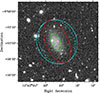 |
Fig. 4. DESI Legacy Survey g-band image of VCC 1964 of 2.5′ F.O.V., with ellipses showing different inclination estimates. Green is the result from the SMUDGES catalogue. The red ellipse shows the aperture we use for photometry on the SDSS data, using the SMUDGES fit but increasing the aperture size by a factor of 2.5 to visually estimate the limit of the galaxy. The cyan ellipses are the same size as the visual fit but with inclination angles that would give a rotation width compatible with the standard (solid) and 2 σ-scatter (dashed) of the BTFR. |
Before commenting further on the potential significance of this, we first describe how the BTFR was constructed. We closely follow the procedure given in the appendix of Taylor et al. (2022) (hereafter T22BTFR); for the sake of space, we only summarise the most essential parts of the process here except where we make any alterations (for a reproduction of the BTFR, we refer to T22BTFR). We note, as in our earlier work, that the McGaugh (2012) objects included in Figure 3 primarily serves as a control sample, demonstrating that the corrections made to our line-width data give results in good agreement with the resolved rotation curves of McGaugh (2012) (that sample consists of galaxies with stellar and gas masses ranging approximately from 106–9 M⊙, with rotation speeds from 17–150 km s−1).
3.4.1. H I measurements
We measured the H I parameters of VCC 1964 using four datasets: the original AGES VC1 data with and without Hanning smoothing, the WAVES cube, and the combined AGES and WAVES data (which we use for the measurements presented here). As noted the WAVES dataset is significantly more noisy (1.9 mJy rms) than the AGES data in this region and therefore we only use the Hanning smoothed data in this case. Hanning smoothing, as used in standard AGES and WAVES data reduction procedures – indeed this is almost ubiquitous in single-dish H I data – averages half the central channel value with one quarter of the adjacent channels, thus degrading our nominal 5 km s−1 resolution to 10 km s−1.
For plotting the BTFR, line widths are corrected for spectral resolution (based on the source S/N) and cosmological broadening exactly as in T22BTFR, as are the corrections for rotation (essentially dependent only on inclination) and the difference between the peak and flat parts of the rotation curve (dependent on stellar mass); see Section 3.4.2. The only difference is that here we have also shown the line width using the unsmoothed data, for which we assume 5 km s−1 resolution when correcting for instrumental broadening. When using unsmoothed data, we also remeasured the total flux using the same data.
We find there is very little scope for error in the measured flux. Except for the pure WAVES cube, we found the flux did not differ by more than 5% of the value presented here, with this value being the lowest of those measured. Only the pure WAVES data gives a flux significantly higher (0.411 Jy km s−1) but this is likely due to the higher noise level, with the effects of noise boosting being well-known (e.g. Hogg & Turner 1998, Deshev et al. 2022). Similarly, line widths never vary significantly, being at most 3 km s−1 less than the reported values in Table 1 – they were never found to be higher than this.
It is important to note that though the shift on the BTFR using the unsmoothed data is small, it is significant, and we caution that the BTFR deviation is susceptible to relatively small measurement changes. Despite this, the strength of the signal is clearly evident in Figure 2, and it is unlikely there is any missing broader component that would shift VCC 1964 to higher line widths. We also note that when we remeasured the spectrum as described in Section 3.2, the line width measurements never exceeded the value given in Table 1. We therefore consider our measured line width an upper limit on the true value.
3.4.2. Optical parameters
The optical parameters of the typical galaxies shown in the BTFR presented here are derived using standard SDSS automated photometry. We would prefer to use this for VCC 1964 to ensure homogeneity, but despite being readily visible in the SDSS data, the photometric measurements in this case are clearly inaccurate. For example the SDSS estimate its apparent g magnitude to be 20.16, whereas SMUDGES (which relies on LS data) finds it to be 17.59. Performing aperture photometry on the SDSS data, visually fitting an aperture in DS9 without reference to the SMUDGES aperture, we found a very similar value to SMUDGES (mg = 17.61). The difference from the SDSS measurement is likely due to the difficulties of algorithmically fitting low surface brightness objects (though we also note that the inclination angle estimates from the SDSS and SMUDGES are virtually identical, with the r band b/a value in the SDSS being 0.50 and the LS value being 0.49, equivalent to 60 and 61° respectively).
To avoid using a purely visual fit to the optical data, and ensure we use the same photometric bands for the stellar mass calculation as in T22BTFR (see below), we adopt the following approach : we use the aperture given in the SMUDGES table but use the SDSS gri data for estimating the magnitudes. We expand this aperture by a factor 2.5 to ensure all the light in each band is captured, hence the difference in the sizes of the ellipses in Figure 4. Point sources visible within the aperture are masked. We use the same ellipses for photometry in the SDSS g, r and i bands. With the apparent magnitudes thus obtained, we apply the same extinction and (numerous) other corrections as described in full T22BTFR.
For comparison, we note that using the aperture purely defined by SMUDGES (including Re) would give a g magnitude 0.84 fainter than with our adjusted aperture. The reason for this is that the SMUDGES magnitudes are extrapolated from the Sérsic profile, and our adjusted size for a Sérsic index of n = 0.51 (as determined by SMUDGES) is expected to enclose > 98% of the light. Given the very close agreement between even our visually estimated aperture and the SMUDGES algorithmic measurements, which used two different datasets, the photometric magnitudes are secure.
A more fundamental problem for the present analysis is the choice of stellar mass prescription. Using the three SDSS bands and the various prescriptions in Bell et al. (2003), Taylor et al. (2011), and Roediger & Courteau (2015), gives a range of possible stellar masses from 5.6×10⁶ M⊙ – 6.4×10⁷ M⊙1. For the value in Table 1 we choose to give the value as used for the BTFR calculation to ensure consistency. This uses the Taylor et al. (2011) prescription for the g–i colour but includes an additional correction to give stellar masses in agreement with the calculations of McGaugh (2012); again see T22BTFR for full details. While the range of stellar masses calculated is large, reassuringly, the value we have used here is almost exactly the median for our eight calculated values using the various prescriptions. We note that all but the most extreme masses are within a factor two of this value. Due to the systematic issues in calculating the stellar mass, we refrain from commenting on the MH I/M* ratio except to estimate the likely range being from 0.3–4.0.
3.5. Effect of the parameter uncertainty on the BTFR deviation
As in T22BTFR, we deliberately avoid giving error bars on the BTFR because the many systematic effects are expected to strongly dominate over the formal measurement errors. In the main, however, the deviation of VCC 1964 from the BTFR is not likely subject to any great uncertainties. The velocity width is robust to our choice of dataset and profile parameters, with the flux at 20% of the peak still being well above the noise level, and the integrated flux level giving consistent results (except for the case of WAVES as already discussed, but this would only increase the deviation). We nevertheless caution that the small difference in widths measured in the standard and unsmoothed AGES cubes does lead to a noticeable difference in the BTFR, although there is no evidence for a missing broader component. The inclination angle is nearly identical as estimated by the SDSS and SMUDGES, and the angle needed to reconcile the line width with the BTFR is clearly incompatible with the data.
There are two potential systematic issues that could affect the deviation more strongly (in addition to the distance, discussed earlier). Firstly, as in T22BTFR we have chosen not to correct for turbulence in calculating the rotation width, for the same reason as given therein: others have chosen to simply subtract 6.5 km s−1 from the line width, but this is a rather large correction for low line width galaxies that could introduce considerable additional uncertainties (though it would only increase the deviation from the BTFR).
Secondly, the range of stellar masses allowed by the data is considerable. In terms of affecting the BTFR, however, the effect of this is likely to be small, as the correction would have to be applied to every galaxy plotted (though, since the extent of this may vary with colour and magnitude, we therefore also show an optical TFR in Section 3.6). More important here is the decision to keep everything self-consistent, so that the deviation can be stated with confidence even if the actual baryonic mass cannot.
We emphasise here that the distance assumption will only have a significant effect if the galaxy is or is not a cluster member. At our assumed distance of 17 Mpc, the effective radius computed in SMUDGES is (equivalently) just one arcsecond short of the nominal 1.5 kpc for UDG classification. With the cluster still in the process of assembly, and clouds infalling from 23 and even 32 Mpc (see AGES V for a discussion), a distance underestimate of 1 Mpc that would increase the physical Re to 1.5 kpc is certainly plausible; Mei et al. (2007) estimate the cluster depth at 2.4 Mpc.
If, on the other hand, VCC 1964 were shown to be well in front of the cluster, then our interpretation would change completely. Jones et al. (2022a) believe the VCC 2037 system is actually at 10 Mpc distance, low enough to reconcile VCC 1964 with the (2σ) observational scatter in the BTFR. Its effective radius would then be 0.8 kpc, placing it well short of the usual UDG criterion. A problem with this scenario is that the VCC 2037 system is approximately 1.4° away in projection, which is 244 kpc at this distance, making a direct association with VCC 1964 unlikely. Furthermore, as we have argued, explaining the displacement of the gas and its low line width would become much more difficult in that scenario. In addition, the velocity of VCC 2037 is 300 km s−1 lower than that of VCC 1964, with VCC 1964 requiring a rather high peculiar velocity of 700 km s−1 with respect to the cluster if it were actually at 10 Mpc – and an even lower distance of 5 Mpc, and so an even higher peculiar velocity, is required to bring VCC 1964 into full agreement with the BTFR.
3.5.1. Effect of gas loss on the TFR deviation
In Taylor et al. (2013) we found that strongly deficient galaxies, which have ≤10% of the H I content of field galaxies of similar morphology and optical diameter (i.e. deficiencies > 1.0), also show anomalously low line widths. We attributed this to gas loss truncating the rotation curve such that the detected H I corresponds to the central, steeply rising part of the curve rather than the outer, flat region. In this scenario the dark matter itself is unaffected: instead, the observable H I would simply not probe as great an extent of the rotation curve as for non-deficient galaxies (this is in strong contrast to some ideas in which UDG formation involves actual dark matter depletion, e.g. Silk 2019).
A difficulty with testing this idea here is that the smooth morphology but blue colour of VCC 1964 makes the deficiency calculation uncertain. To explain why, we recall the procedure for calculating deficiency. H I deficiency is defined in Giovanelli & Haynes (1983) as
 (3)
(3)
Since this is a logarithmic quantity, a deficiency of 1.0 means a galaxy has lost 90% of its original gas content, a deficiency of 2.0 implies a loss of 99%, etc. The expected gas content is defined as
 (4)
(4)
where a and b are coefficients derived from a sample of isolated field galaxies (where environmental effects are believed to be minimal). Traditionally these are defined based on the Hubble-type morphology of the galaxy in combination with its optical diameter in kpc (d); the problem with VCC 1964 being that its smooth structure but blue colour make it uncertain which values of a and b we should adopt (this was why it was excluded from the TFR plots in our earlier papers). In addition, various studies have come up with different values for these coefficients. Using the same parameters (as Solanes et al. 1996 to calculate the deficiency, as we used in Taylor et al. 2013), we calculated the deficiency to be 0.73 for the generalised values and 0.48 for a dwarf irregular or later type (i.e. the galaxy retains 19 or 33% of its expected original gas content, respectively)2.
Thus, comparing to our previous findings, it does not appear likely that VCC 1964 has lost sufficient gas to truncate its rotation curve (suggesting its dynamics are indeed intrinsically unusual) – with the important caveat that the stripping may still have affected its line width by perturbing the object from equilibrium, rather than truncating its rotation curve. We stress here that regardless of the cause, deviations from the BTFR (even in Virgo) are rare among ‘normal’ galaxies (with the dynamics of UDGs still being under dispute). Such similar deviations as we saw in Virgo were only for a very few, much brighter galaxies than VCC 1964 of extreme deficiency, and we saw no evidence of any correlation with deficiency with BTFR offset. Whatever the cause of the deviation it must be an unusual mechanism. On the other hand, VCC 1964 clearly is an unusual object, and there are few if any other objects that allow for comparisons. We return to this point in the discussion.
3.6. Alternative optical TFR
While the deviation from the computed BTFR appears robust to measurement errors and stellar mass estimates, as an additional test we also construct an optical version of the TFR. We follow the prescription of Kourkchi et al. (2020) (K20), who calibrate the TFR using over 10 000 spiral galaxies with SDSS, WISE, and ALFALFA data. Using an optical form of the TFR has the advantage of avoiding the large variations possible from stellar mass recipes, and the K20 method also includes a more sophisticated correction (as opposed to linearly subtracting a constant value) for turbulence in the line width. Below we give only a brief summary of our corrections to ensure reproducibility (the physical basis of this approach was presented by K20).
The optical TFR is constructed as follows. The correction for Galactic extinction is done in the same way as for the BTFR. Lacking the WISE photometry used in K20, we follow their colour-adjusted method. First, after correcting for Galactic extinction and applying a K-correction, apparent magnitudes are converted to pseudo-magnitudes as per their Equations (16)–(18),

where Cg is a pseudo-magnitude that in effect corrects for internal extinction, converted into an absolute magnitude using the standard procedure.
Line widths are corrected as follows (following the procedure of Courtois et al. (2009), as adopted in K20; we give the equations here in their formalism). Our W20 values, measured using the peak flux, are converted to the W50 range that encloses 90% of the total H I flux,

These were corrected for redshift and resolution as

The correction for turbulence is given by


where k1 and k2 are the constants 100 km s−1 and 9 km s−1, respectively. Finally, we corrected for inclination using the same values as in the BTFR, using the full line width (rather than half) for consistency with K20. We plot their optical TFR,

where Mg is the pseudo-absolute-magnitude, with K20 giving a 1σ scatter in this relation of 0.48. Our result is shown in Figure 5. The deviation of VCC 1964 increases significantly to over 6σ. We submit that while the physical interpretation of this is certainly an open question (primarily the issue is whether this reflects the intrinsic dynamics of the galaxy or is a result of the gas – quite literally – being pushed out of equilibrium), the deviation itself is clear.
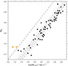 |
Fig. 5. Optical form of the TFR following the method of K20. Black points are our AGES galaxies, with VCC 1964 highlighted in orange (as in Figure 3 the orange square uses H I data without Hanning smoothing). The solid line is the relation obtained in K20 with the dashed and dotted lines showing their estimated 1 and 2σ scatter. The upper dashed line shows the 6σ deviation. |
3.7. Other TFR caveats
The final issue that is relevant for understanding this object is the unresolved nature of the H I detection. A resolved rotation curve would show whether the H I line width is really probing the flat part of the curve or if this has perhaps been truncated (or otherwise affected) by the assumed ram pressure stripping. Additionally, since we can only constrain the H I size to be less than the Arecibo beam size (17 kpc at the Virgo distance), we cannot give an estimate of the dynamical mass with any meaningful precision. If the rotation curve is flat then the deviation from the BTFR indicates a deficit of dark matter compared to typical galaxies, but without a radius for the H I, we cannot say how much. For comparison, if the line width were within the 2σ BTFR scatter or in perfect agreement with the McGaugh (2012) relation, this would imply a dynamical mass 2–4 times greater than its present value. More generally, a resolved H I map could show if the gas has ordered motions or if the stripping has disturbed it from equilibrium, which might invalidate the BTFR interpretations. Numerical modelling could also be used to investigate if and how the gas rotation changes when displaced from its parent galaxy.
We have discussed the possibility of an inaccurate distance estimate in Section 3.5, noting that 10 Mpc – the same as Jones et al. (2022a) measured for NGVS 3543, and also for VCC 2037 in Karachentsev et al. 2014 – would bring VCC 1964 within the observed scatter in the BTFR. We find this unlikely due to the high peculiar velocity this would imply for VCC 1964, its large separation from the system described in Jones et al. (2022a), and the lack of an obvious cause of gas removal in this scenario. We add here two additional points. First, Jones et al. (2022a) identified a much larger H I stream as the source of the gas and there were multiple optical structures in close proximity to NGVS 3543. No such features are apparent around VCC 1964. Furthermore the prospect of a second candidate UDG projected against Virgo, with a similarly adjacent but actually unrelated gas cloud, is highly improbable. Of course, only a robust distance measurement to VCC 1964 could fully settle the dilemma, though we note that such estimates are sometimes far from clear-cut – see the introduction of Beasley et al. (2025) for a summary of a particularly well-known example. Second, while it is possible that VCC 1964 is actually at a larger distance (say within the 23 or 32 Mpc) cloud, this would not change the estimate line width but would increase its inferred baryonic mass, thus only making the BTRF-discrepancy more pronounced.
In short, while there are legitimate questions as to the precise numerical values for all parameters, there is little indication that this could change any of the major conclusions presented here. Uncertainties of the velocity width are small, and the estimated width is likely an overestimate due to turbulence (resolved H I observations would greatly help with this). The inclination angle is consistent between two independent datasets and incompatible with bringing the line width into agreement with the BTFR. The offset of the optical and H I position is robust in two independent datasets, albeit again better resolution would be of benefit here. The stellar mass estimate is subject to a larger uncertainty, but this would affect other galaxies on the BTFR so is very unlikely to explain the deviation of VCC 1964.
4. Discussion
VCC 1964 is a candidate for a UDG that is losing gas in the Virgo cluster as a result of ram-pressure stripping. The displacement of its gas and stellar component are well aligned with the vector towards M49, which is the centre of the local maximum of X-ray gas. Conversely, there are no other plausible sources of the H I gas within 250 kpc, and the simple offset from the optical counterpart does not match expectations from a tidal encounter. In that case, we would (typically) expect the gas to be asymmetrically disturbed around the centre of mass, rather than displaced wholesale.
We note one other candidate for a Virgo cluster UDG that currently experiences the onset of ram pressure. Junais et al. (2022) selected a sample of LSB galaxies from the Next Generation Virgo Survey, five of which are detected in H I from ALFALFA. The authors stated that this does not include any of their 26 LSB galaxies that they identified as UDGs, but they defined UDGs using the more complex criteria of Lim et al. (2020). Based on the standard effective radius and surface brightness criteria (see Lim et al. 2020, Table 2), two of their H I detections would be classified as UDGS: VCC 169 and AGC 220597. The authors noted the former as possibly suggestive of the onset of ram-pressure stripping based on its Hα detection. This object is also detected in WAVES. We will comment further on this in the final WAVES catalogue paper, but we note here that it does not show any offset between the H I and optical positions, nor any disturbances in its H I contours; it may be in an earlier stage of stripping than VCC 1964. The highly irregular optical morphology of the object makes any estimate of its inclination angle difficult, and we therefore cannot comment on its position on the BTFR.
Recently, Dey et al. (2025) have built on the work of Jones et al. (2022b) to describe a class of stellar systems in Virgo they called ‘blue blobs’. They interpreted these as ram-pressure dwarfs, analogous to tidal dwarfs, but with a ram-pressure origin of the gas rather than tidal interactions. Numerical simulations in Calura et al. (2020) showed that these objects could be gravitationally self-bound and stable on long (> 1 Gyr) timescales. If in the cluster, VCC 1964 almost certainly has a stellar mass that is considerably greater than most of the known blue blobs (median 1.3 × 10⁵ M⊙ from the catalogue of Dey et al. 2025), but the same principle could apply, with its stellar mass being recently formed within the H I. On the other hand, the smooth, symmetrical nature of VCC 1964 is not obviously consistent with this, and neither is the offset between the H I and the optical components.
The offset of VCC 1964 from the BTFR can be reconciled by a distance of 10 Mpc, the same as was measured for VCC 2034 (Jones et al. 2022a) – but in that case the lack of nearby galaxies would then make its displaced gas difficult to explain. If in Virgo, the offset from the BTFR is also not necessarily problematic, as this has been shown to be the case for many other UDGs. Detailed hydrodynamic studies are needed to show whether a galaxy like this would retain its very narrow H I line width, or indeed if the removal is itself the cause of the narrow line, and also to address whether the stellar disc would remain undisturbed (as it appears to be) during the removal of the relatively massive gas component. This is particularly significant given its apparent deficit of dark matter.
The interpretation of the offset of VCC 1964 is much the most uncertain aspect of our analysis. We have previously shown examples of objects with similar offsets due to a truncation of the H I disc (i.e. the measured line width), but the deficiency of this object is not consistent with this. Despite this, the gas may not be in stable rotation, as the BTFR assumes, and indeed, that the gas is displaced is certainly evidence of this. The issue here is the great uncertainty regarding what happens to the line width of stripped gas. Many objects have a truncated rotation curve of the remaining gas, but with significantly larger widths in the stripped material (e.g. Kenney et al. (2004), Ignesti et al. (2024), Fossati et al. (2016)). In simulations of tidal stripping, Taylor et al. (2017) found that stripped gas tends to increase in line width. Of most direct relevance, Luo et al. (2023) reported that the velocity dispersion of stripped Hα tails increases through turbulent mixing with the ICM. This implies that the material that remains in the disc, despite its currently lower line width, would increase in width on its removal into the ICM.
Since the gas appears to have been wholly removed from the disc of VCC 1964, the above could be taken to indicate that we are, if anything, overestimating its line width, but there are many caveats. The tail widths in Luo et al. (2023) increase on scales of 20 kpc, whereas the gas of VCC 1964 is only offset by 9 kpc. More significantly, the Luo et al. (2023) tails show strong local variations in velocity dispersion, not a smooth linear increase. The situation of VCC 1964 is also different in that this appears to be far more of a case of gas displacement rather than continuous deformation into an elongated tail. Without similar galaxies for comparison (and/or detailed hydrodynamical modelling), the expected change in line width is far from obvious.
We have also described how UDGs differ substantially in terms of their GC populations, and it is therefore hard to generalise how this one particular example relates to UDGs in clusters more widely. Indeed, its very peculiarities are what make this a remarkable system. It has the lowest H I mass detected in a UDG to date, and the displaced from its stellar component through the optical emission is smooth, with the H I detected closer to the local cluster centre than the stars. Explaining this collective strangeness, together with its TFR offset, remains challenging.
A direct distance measurement is needed to determine whether VCC 1964 really is a UDG that enters the Virgo cluster for the first time. If this is the case, it would suggest that gas-depleted cluster UDGs (the majority found so far) can form from the gas-rich population known in the field. This implies a common (though poorly constrained so far) origin for at least some members of both types of object. VCC 1964 itself is just one object, and it is conceivable that multiple formation pathways are still at work. Only larger sample sizes can address this issue and help us to understand the formation of similar objects that apparently lack dark matter.
Data availability
The AGESVC1 data cube is available in its entirety on request to the corresponding author. The full WAVES cube is awaiting publication, but the combined AGES-WAVES data set used here can be similarly made available on request. All other data sources used in this work are public.
Acknowledgments
We thank our numerous colleagues at the ASU for their helpful and productive discussions. We also thank the anonymous referee whose comments have significantly improved the manuscript. This work was supported by the institutional project RVO:67985815, the Czech Ministry of Education, Youth and Sports from the large infrastructures for Research, Experimental Development and Innovations project LM 2015067, and the Charles University project GA UK No. 376425. This research has made use of the SDSS. Funding for the Sloan Digital Sky Survey V has been provided by the Alfred P. Sloan Foundation, the Heising-Simons Foundation, the National Science Foundation, and the Participating Institutions. SDSS acknowledges support and resources from the Center for High-Performance Computing at the University of Utah. SDSS telescopes are located at Apache Point Observatory, funded by the Astrophysical Research Consortium and operated by New Mexico State University, and at Las Campanas Observatory, operated by the Carnegie Institution for Science. The SDSS web site is www.sdss.org. SDSS is managed by the Astrophysical Research Consortium for the Participating Institutions of the SDSS Collaboration, including the Carnegie Institution for Science, Chilean National Time Allocation Committee (CNTAC) ratified researchers, Caltech, the Gotham Participation Group, Harvard University, Heidelberg University, The Flatiron Institute, The Johns Hopkins University, L’Ecole polytechnique fédérale de Lausanne (EPFL), Leibniz-Institut für Astrophysik Potsdam (AIP), Max-Planck-Institut für Astronomie (MPIA Heidelberg), Max-Planck-Institut für Extraterrestrische Physik (MPE), Nanjing University, National Astronomical Observatories of China (NAOC), New Mexico State University, The Ohio State University, Pennsylvania State University, Smithsonian Astrophysical Observatory, Space Telescope Science Institute (STScI), the Stellar Astrophysics Participation Group, Universidad Nacional Autónoma de México (UNAM), University of Arizona, University of Colorado Boulder, University of Illinois at Urbana-Champaign, University of Toronto, University of Utah, University of Virginia, Yale University, and Yunnan University.
References
- Auld, R., Minchin, R. F., Davies, J. I., et al. 2006, MNRAS, 371, 1617 [NASA ADS] [CrossRef] [Google Scholar]
- Barnes, D. G., Staveley-Smith, L., de Blok, W. J. G., et al. 2001, MNRAS, 322, 486 [Google Scholar]
- Beasley, M. A., Romanowsky, A. J., Pota, V., et al. 2016, ApJ, 819, L20 [NASA ADS] [CrossRef] [Google Scholar]
- Beasley, M. A., Fahrion, K., Guerra Arencibia, S., Gvozdenko, A., & Montes, M. 2025, A&A, 697, A144 [NASA ADS] [CrossRef] [EDP Sciences] [Google Scholar]
- Bell, E. F., McIntosh, D. H., Katz, N., & Weinberg, M. D. 2003, ApJS, 149, 289 [Google Scholar]
- Benavides, J. A., Sales, L. V., Abadi, M. G., et al. 2021, Nat. Astron., 5, 1255 [NASA ADS] [CrossRef] [Google Scholar]
- Binggeli, B., Sandage, A., & Tammann, G. A. 1985, AJ, 90, 1681 [Google Scholar]
- Buzzo, M. L., Forbes, D. A., Jarrett, T. H., et al. 2025, MNRAS, 536, 2536 [Google Scholar]
- Calura, F., Bellazzini, M., & D’Ercole, A. 2020, MNRAS, 499, 5873 [Google Scholar]
- Conselice, C. J. 2018, RNAAS, 2, 43 [NASA ADS] [Google Scholar]
- Courtois, H. M., Tully, R. B., Fisher, J. R., et al. 2009, AJ, 138, 1938 [Google Scholar]
- Cramer, W. J., Kenney, J. D. P., Cortes, J. R., et al. 2020, ApJ, 901, 95 [NASA ADS] [CrossRef] [Google Scholar]
- Davies, J. I., Auld, R., Burns, L., et al. 2011, MNRAS, 415, 1883 [NASA ADS] [CrossRef] [Google Scholar]
- Deshev, B., Taylor, R., Minchin, R., Scott, T. C., & Brinks, E. 2022, A&A, 665, A155 [NASA ADS] [CrossRef] [EDP Sciences] [Google Scholar]
- Dey, A., Schlegel, D. J., Lang, D., et al. 2019, AJ, 157, 168 [Google Scholar]
- Dey, S., Jones, M. G., Sand, D. J., et al. 2025, ApJ, 983, 2 [Google Scholar]
- di Serego Alighieri, S., Gavazzi, G., Giovanardi, C., et al. 2007, A&A, 474, 851 [NASA ADS] [CrossRef] [EDP Sciences] [Google Scholar]
- Durbala, A., Finn, R. A., Crone Odekon, M., et al. 2020, AJ, 160, 271 [NASA ADS] [CrossRef] [Google Scholar]
- Forbes, D. A., Alabi, A., Romanowsky, A. J., Brodie, J. P., & Arimoto, N. 2020, MNRAS, 492, 4874 [Google Scholar]
- Fossati, M., Fumagalli, M., Boselli, A., et al. 2016, MNRAS, 455, 2028 [Google Scholar]
- Gavazzi, G., Boselli, A., Scodeggio, M., Pierini, D., & Belsole, E. 1999, MNRAS, 304, 595 [Google Scholar]
- Gavazzi, G., Boselli, A., Donati, A., Franzetti, P., & Scodeggio, M. 2003, A&A, 400, 451 [NASA ADS] [CrossRef] [EDP Sciences] [Google Scholar]
- Giovanelli, R., & Haynes, M. P. 1983, AJ, 88, 881 [Google Scholar]
- Giovanelli, R., Haynes, M. P., Kent, B. R., et al. 2005, AJ, 130, 2598 [Google Scholar]
- Grishin, K. A., Chilingarian, I. V., Afanasiev, A. V., et al. 2021, Nat. Astron., 5, 1308 [NASA ADS] [CrossRef] [Google Scholar]
- Grossi, M., Corbelli, E., Bizzocchi, L., et al. 2016, A&A, 590, A27 [NASA ADS] [CrossRef] [EDP Sciences] [Google Scholar]
- Hartke, J., Iodice, E., Gullieuszik, M., et al. 2025, A&A, 695, A91 [NASA ADS] [CrossRef] [EDP Sciences] [Google Scholar]
- Haynes, M. P., Giovanelli, R., Kent, B. R., et al. 2018, ApJ, 861, 49 [Google Scholar]
- Hogg, D. W., & Turner, E. L. 1998, PASP, 110, 727 [NASA ADS] [CrossRef] [Google Scholar]
- Hu, H.-J., Guo, Q., Zheng, Z., et al. 2023, ApJ, 947, L9 [NASA ADS] [CrossRef] [Google Scholar]
- Ignesti, A., Brunetti, G., Gullieuszik, M., et al. 2024, ApJ, 977, 219 [Google Scholar]
- Jáchym, P., Kenney, J. D. P., Sun, M., et al. 2019, ApJ, 883, 145 [Google Scholar]
- Janowiecki, S., Jones, M. G., Leisman, L., & Webb, A. 2019, MNRAS, 490, 566 [NASA ADS] [CrossRef] [Google Scholar]
- Jones, M. G., Sand, D. J., Bellazzini, M., et al. 2022a, ApJ, 926, L15 [NASA ADS] [CrossRef] [Google Scholar]
- Jones, M. G., Sand, D. J., Bellazzini, M., et al. 2022b, ApJ, 935, 51 [Google Scholar]
- Jones, M. G., Karunakaran, A., Bennet, P., et al. 2023, ApJ, 942, L5 [CrossRef] [Google Scholar]
- Junais, Boissier, S., Boselli, A., et al. 2021, A&A, 650, A99 [NASA ADS] [CrossRef] [EDP Sciences] [Google Scholar]
- Junais, Boissier, S., Boselli, A., et al. 2022, A&A, 667, A76 [NASA ADS] [CrossRef] [EDP Sciences] [Google Scholar]
- Kado-Fong, E., Kim, C.-G., Greene, J. E., & Lancaster, L. 2022, ApJ, 939, 101 [NASA ADS] [CrossRef] [Google Scholar]
- Karachentsev, I. D., Tully, R. B., Wu, P.-F., Shaya, E. J., & Dolphin, A. E. 2014, ApJ, 782, 4 [NASA ADS] [CrossRef] [Google Scholar]
- Karunakaran, A., Spekkens, K., Zaritsky, D., et al. 2020, ApJ, 902, 39 [CrossRef] [Google Scholar]
- Karunakaran, A., Motiwala, K., Spekkens, K., et al. 2024, ApJ, 975, 91 [Google Scholar]
- Keenan, O. C., Davies, J. I., Taylor, R., & Minchin, R. F. 2016, MNRAS, 456, 951 [NASA ADS] [CrossRef] [Google Scholar]
- Kenney, J. D. P., van Gorkom, J. H., & Vollmer, B. 2004, AJ, 127, 3361 [Google Scholar]
- Koda, J., Yagi, M., Yamanoi, H., & Komiyama, Y. 2015, ApJ, 807, L2 [NASA ADS] [CrossRef] [Google Scholar]
- Kourkchi, E., Tully, R. B., Anand, G. S., et al. 2020, ApJ, 896, 3 [NASA ADS] [CrossRef] [Google Scholar]
- Leisman, L., Haynes, M. P., Janowiecki, S., et al. 2017, ApJ, 842, 133 [NASA ADS] [CrossRef] [Google Scholar]
- Leroy, A., Bolatto, A. D., Simon, J. D., & Blitz, L. 2005, ApJ, 625, 763 [NASA ADS] [CrossRef] [Google Scholar]
- Lim, S., Côté, P., Peng, E. W., et al. 2020, ApJ, 899, 69 [CrossRef] [Google Scholar]
- Luo, R., Sun, M., Jáchym, P., et al. 2023, MNRAS, 521, 6266 [NASA ADS] [CrossRef] [Google Scholar]
- Mancera Piña, P. E., Fraternali, F., Adams, E. A. K., et al. 2019, ApJ, 883, L33 [CrossRef] [Google Scholar]
- Mancera Piña, P. E., Fraternali, F., Oman, K. A., et al. 2020, MNRAS, 495, 3636 [Google Scholar]
- Martínez-Delgado, D., Cooper, A. P., Román, J., et al. 2023, A&A, 671, A141 [NASA ADS] [CrossRef] [EDP Sciences] [Google Scholar]
- McGaugh, S. S. 2012, AJ, 143, 40 [Google Scholar]
- McGaugh, S. S., Schombert, J. M., Bothun, G. D., & de Blok, W. J. G. 2000, ApJ, 533, L99 [Google Scholar]
- Mei, S., Blakeslee, J. P., Côté, P., et al. 2007, ApJ, 655, 144 [Google Scholar]
- Minchin, R. F., Momjian, E., Auld, R., et al. 2010, AJ, 140, 1093 [NASA ADS] [CrossRef] [Google Scholar]
- Minchin, R. F., Taylor, R., Köppen, J., et al. 2019, AJ, 158, 121 [NASA ADS] [CrossRef] [Google Scholar]
- Moreno, J., Danieli, S., Bullock, J. S., et al. 2022, Nat. Astron., 6, 496 [NASA ADS] [CrossRef] [Google Scholar]
- Oman, K. A., Navarro, J. F., Sales, L. V., et al. 2016, MNRAS, 460, 3610 [Google Scholar]
- Papastergis, E., Adams, E. A. K., & Romanowsky, A. J. 2017, A&A, 601, L10 [NASA ADS] [CrossRef] [EDP Sciences] [Google Scholar]
- Roediger, J. C., & Courteau, S. 2015, MNRAS, 452, 3209 [NASA ADS] [CrossRef] [Google Scholar]
- Román, J., & Trujillo, I. 2017, MNRAS, 468, 4039 [Google Scholar]
- Saifollahi, T., Trujillo, I., Beasley, M. A., Peletier, R. F., & Knapen, J. H. 2021, MNRAS, 502, 5921 [NASA ADS] [CrossRef] [Google Scholar]
- Saintonge, A. 2007, AJ, 133, 2087 [NASA ADS] [CrossRef] [Google Scholar]
- Sandoval Ascencio, L., Cooper, M. C., Zaritsky, D., et al. 2025, Open J. Astrophys., 8, 110 [Google Scholar]
- Sault, R. J., Teuben, P. J., & Wright, M. C. H. 1995, ASP Conf. Ser., 77, 433 [NASA ADS] [Google Scholar]
- Shen, Z., van Dokkum, P., & Danieli, S. 2023, ApJ, 957, 6 [NASA ADS] [CrossRef] [Google Scholar]
- Shi, D. D., Zheng, X. Z., Zhao, H. B., et al. 2017, ApJ, 846, 26 [Google Scholar]
- Silk, J. 2019, MNRAS, 488, L24 [NASA ADS] [CrossRef] [Google Scholar]
- Solanes, J. M., Giovanelli, R., & Haynes, M. P. 1996, ApJ, 461, 609 [Google Scholar]
- Spekkens, K., & Karunakaran, A. 2018, ApJ, 855, 28 [NASA ADS] [CrossRef] [Google Scholar]
- Sun, Y.-Z., Zhang, H.-X., Brinks, E., et al. 2025, A&A, 701, A73 [NASA ADS] [CrossRef] [EDP Sciences] [Google Scholar]
- Taylor, R. 2010, Ph.D. Thesis, Cardiff University, UK [Google Scholar]
- Taylor, R. 2015, Astron. Comput., 13, 67 [NASA ADS] [CrossRef] [Google Scholar]
- Taylor, R. 2025a, Astron. Comput., 51, 100927 [NASA ADS] [CrossRef] [Google Scholar]
- Taylor, R. 2025b, A&A, 696, A113 [NASA ADS] [CrossRef] [EDP Sciences] [Google Scholar]
- Taylor, E. N., Hopkins, A. M., Baldry, I. K., et al. 2011, MNRAS, 418, 1587 [Google Scholar]
- Taylor, R., Davies, J. I., Auld, R., & Minchin, R. F. 2012, MNRAS, 423, 787 [NASA ADS] [CrossRef] [Google Scholar]
- Taylor, R., Davies, J. I., Auld, R., Minchin, R. F., & Smith, R. 2013, MNRAS, 428, 459 [NASA ADS] [CrossRef] [Google Scholar]
- Taylor, R., Minchin, R. F., Herbst, H., et al. 2014, MNRAS, 443, 2634 [NASA ADS] [CrossRef] [Google Scholar]
- Taylor, R., Davies, J. I., Jáchym, P., et al. 2017, MNRAS, 467, 3648 [Google Scholar]
- Taylor, R., Köppen, J., Jáchym, P., et al. 2020, AJ, 159, 218 [NASA ADS] [CrossRef] [Google Scholar]
- Taylor, R., Köppen, J., Jáchym, P., et al. 2022, AJ, 164, 233 [NASA ADS] [CrossRef] [Google Scholar]
- van Dokkum, P. G., Abraham, R., Merritt, A., et al. 2015, ApJ, 798, L45 [NASA ADS] [CrossRef] [Google Scholar]
- van Dokkum, P., Abraham, R., Brodie, J., et al. 2016, ApJ, 828, L6 [Google Scholar]
- van Dokkum, P., Danieli, S., Cohen, Y., et al. 2018, Nature, 555, 629 [Google Scholar]
- van Dokkum, P., Danieli, S., Abraham, R., Conroy, C., & Romanowsky, A. J. 2019, ApJ, 874, L5 [Google Scholar]
- Westmeier, T., Kitaeff, S., Pallot, D., et al. 2021, MNRAS, 506, 3962 [NASA ADS] [CrossRef] [Google Scholar]
- Yagi, M., Yoshida, M., Komiyama, Y., et al. 2010, AJ, 140, 1814 [Google Scholar]
- Yagi, M., Yoshida, M., Gavazzi, G., et al. 2017, ApJ, 839, 65 [NASA ADS] [CrossRef] [Google Scholar]
- Zaritsky, D., Donnerstein, R., Dey, A., et al. 2023, ApJS, 267, 27 [NASA ADS] [CrossRef] [Google Scholar]
We provide a simple stellar mass calculator at the following URL: https://photcalc.streamlit.app/
We provide a simple online deficiency calculator, with a, b coefficients from multiple sources, at the following URL: https://rhysyt-hicalculators-hidefcal-qqnsnn.streamlit.app/
All Tables
Selected properties of VCC 1964 and its associated H I detection (see text for details).
All Figures
|
Fig. 1. Renzogram of 3.5σ H I contours of VCC 1964 from the combined AGES/WAVES datasets, overlaid on an LS RGB image. The white square and cross mark the positions of the H I centroid and optical position of the galaxy, respectively. The white arrows show the direction vectors to the giant ellipticals M87 and M49, the centre of the main body of the cluster, and the local sub-group. The whole image is 15′ across and ≈75 kpc at the assumed distance of 17 Mpc. The inset images show the same close-up field of view of VCC 1964, with the optical LS data on the left, and GALEX UV on the right. |
| In the text | |
|
Fig. 2. H I spectra of VCC 1964 from AGES (blue), WAVES (red), and the combination (black). The circles and squares show the fitted W50 and W20 velocity widths, respectively. |
| In the text | |
|
Fig. 3. Baryonic Tully-Fisher as in Taylor et al. (2022). The filled black circles use AGES H I data and SDSS photometry, from the H I detected in the background of the Virgo fields and cluster members with deficiencies < 0.6. The open circles are from Table 1 in McGaugh (2012). VCC 1964 is highlighted in orange using the H I data with (circle) and without (square) Hanning smoothing. The filled grey squares show the galaxies in Mancera Piña et al. 2019. Outwards from the solid line, the dashed and dotted lines show the 1, 2, and 4 σ scatter. |
| In the text | |
|
Fig. 4. DESI Legacy Survey g-band image of VCC 1964 of 2.5′ F.O.V., with ellipses showing different inclination estimates. Green is the result from the SMUDGES catalogue. The red ellipse shows the aperture we use for photometry on the SDSS data, using the SMUDGES fit but increasing the aperture size by a factor of 2.5 to visually estimate the limit of the galaxy. The cyan ellipses are the same size as the visual fit but with inclination angles that would give a rotation width compatible with the standard (solid) and 2 σ-scatter (dashed) of the BTFR. |
| In the text | |
|
Fig. 5. Optical form of the TFR following the method of K20. Black points are our AGES galaxies, with VCC 1964 highlighted in orange (as in Figure 3 the orange square uses H I data without Hanning smoothing). The solid line is the relation obtained in K20 with the dashed and dotted lines showing their estimated 1 and 2σ scatter. The upper dashed line shows the 6σ deviation. |
| In the text | |
Current usage metrics show cumulative count of Article Views (full-text article views including HTML views, PDF and ePub downloads, according to the available data) and Abstracts Views on Vision4Press platform.
Data correspond to usage on the plateform after 2015. The current usage metrics is available 48-96 hours after online publication and is updated daily on week days.
Initial download of the metrics may take a while.