| Issue |
A&A
Volume 707, March 2026
|
|
|---|---|---|
| Article Number | A41 | |
| Number of page(s) | 15 | |
| Section | Planets, planetary systems, and small bodies | |
| DOI | https://doi.org/10.1051/0004-6361/202557554 | |
| Published online | 02 March 2026 | |
Revisiting the exoplanet radius valley with host stars from SWEET-Cat
1
Department of Physics, Faculty of Science, Kyambogo University,
PO Box 1,
Kyambogo
Uganda
2
Max-Planck-Institut für Astrophysik,
Karl-Schwarzschild-Str. 1,
85748
Garching
Germany
3
Instituto de Astrofísica e Ciências do Espaço, Universidade do Porto,
Rua das Estrelas,
4150-762
Porto
Portugal
4
Departamento de Física e Astronomia, Faculdade de Ciências da Universidade do Porto,
Rua do Campo Alegre, s/n,
4169-007
Porto
Portugal
5
Max-Planck-Institut für Sonnensystemforschung,
Justus-von-Liebig-Weg 3,
37077
Göttingen
Germany
6
INAF-IAPS,
Via del Fosso del Cavaliere 100,
00133
Roma
Italy
7
Department of Physics, Mbarara University of Science and Technology,
PO Box 1410,
Mbarara
Uganda
★ Corresponding author: This email address is being protected from spambots. You need JavaScript enabled to view it.
Received:
3
October
2025
Accepted:
13
January
2026
Abstract
Context. The radius valley, a deficit in the number of planets with radii around 2 R⊕, was observed among exoplanets that have sizes of ≲5 R and orbital periods of <100 days by NASA’s Kepler mission. This feature separates two distinct populations: super-Earths (rocky planets with radii ≲1.9 R⊕) and sub-Neptunes (planets with substantial volatile envelopes and radii ≳2 R⊕). The valley has been proposed to stem from either planet formation conditions or evolutionary atmospheric loss processes. Disentangling these mechanisms has led to numerous studies of population-level trends, although the resulting interpretations remain sensitive to sample selection and the robustness of host-star parameters.
Aims. Our aim is to re-examine the existence and depth of the radius valley, and how its location varies with orbital period, incident flux, stellar mass, and stellar age.
Methods. We derived robust fundamental stellar parameters of 1221 main-sequence stars (hosting 1405 confirmed planets) from the SWEET-Cat database using a grid-based machine-learning tool (MAISTEP), which incorporates effective temperatures and metallic-ities from spectroscopy, as well as Gaia-based luminosities. Our analysis covers stars with effective temperatures between 4400 and 7500 K (FGK spectral types) and estimated radii between 0.62 and 2.75 R⊕. We attained a median uncertainty of 2% in both stellar radius and stellar mass. Combining the updated stellar radii with planet-to-star radius ratios from the NASA Exoplanet Archive, we recomputed the planetary radii, achieving a median uncertainty of 5%.
Results. Our findings confirm a partially filled planet radius valley near 2 R⊕. The valley depends on the orbital period, incident flux, and stellar mass, with slopes of −0.12−0.01+0.02, 0.10−0.03+0.02, 0.19−0.07+0.09, respectively. We also find a stronger mass-dependent trend in average sizes of sub-Neptunes than super-Earths of slopes 0.17−0.04+0.04 and 0.11−0.05+0.05, respectively. With stellar age, the super-Earth/sub-Neptune number ratio increases from 0.51−0.08+0.11 (<3 Gyr) to 0.64−0.11+0.11 (≥3 Gyr). In addition, the valley becomes shallower and shifts to larger radii, indicating age-dependent evolution in planet sizes. A four-dimensional (planet radius, orbital period, stellar mass, and stellar age) linear fit of the valley in log-log space produces slopes in orbital period and stellar mass that are consistent with the results from the two-dimensional analyses, and a weaker slope of 0.07−0.04+0.03 in stellar age.
Conclusions. The valley’s shift and shallowing over gigayear timescales point to prolonged atmospheric loss, which is consistent with a core-powered mass-loss scenario. Our findings also highlight the importance of stellar age in the interpretation of exoplanet demographics and motivate improved age determinations, as is expected from future missions such as PLATO.
Key words: planet-star interactions / stars: fundamental parameters / planetary systems / stars: solar-type
© The Authors 2026
 Open Access article, published by EDP Sciences, under the terms of the Creative Commons Attribution License (https://creativecommons.org/licenses/by/4.0), which permits unrestricted use, distribution, and reproduction in any medium, provided the original work is properly cited.
This article is published in open access under the Subscribe to Open model. This email address is being protected from spambots. You need JavaScript enabled to view it. to support open access publication.
1 Introduction
Observations from NASA’s Kepler mission revealed more than 4000 exoplanets, most with sizes of ≲5 R⊕ and orbital periods of <100 days (Borucki et al. 2010). A notable feature of this population is a bimodal distribution in the planetary radii, with peaks near ~ 1.5 and ~2.4 R⊕ (Fulton et al. 2017). The region in between these peaks is referred to as the ‘radius gap’ or ‘radius valley’.
The radius valley was not apparent in the initial Kepler data due to large uncertainties in the stellar radii, with typical median errors of ~25% (Huber et al. 2014). A subsequent improvement in stellar characterisation from the California-Kepler Survey (CKS; Johnson et al. 2017; Petigura et al. 2017) reduced the uncertainties significantly. Fulton et al. (2017) reported a median uncertainty of 11% in stellar radii for the CKS sample, translating to a 12% uncertainty in planetary radii. This level of precision allowed for the first observational measurement of a valley among close-in planets, uncovering a key demographic feature in the Kepler observations.
Following this detection, the question of whether the radius valley is truly devoid of planets or partially populated gained attention. In Fulton et al. (2017), the reported planet radius uncertainties of ~12% in their selected CKS sample of 900 planets, limited to host stars with temperatures between 4700 and 6500 K, were comparable to the valley’s width, making it difficult to determine whether the gap was intrinsically empty. Based on asteroseismic stellar radii with a median fractional uncertainty of 2.2% and the corresponding planetary radii with a median uncertainty of 3.3%, Van Eylen et al. (2018) found the valley to be wider and emptier. However, their result may have been influenced by the relatively small sample size of 117 planets. In another study incorporating Gaia DR2 parallaxes, Fulton & Petigura (2018) improved stellar radius measurements to 3%, achieving 5% precision in planetary radii for ~1000 planets, and found the valley to be populated, a conclusion further supported by their simulations. Later, Petigura (2020) revisited the question and argued that many planets near the valley have poorly constrained radii due to significant uncertainties in their measured planet-star radius ratios, an issue common among planets transiting at high impact parameters (b ≳ 0.8), suggesting that the valley may, in fact, be largely empty. Resolving the nature of the radius valley is pivotal in refining models of planetary formation and evolution developed to explain its existence.
To account for this feature in the exoplanet population, several mechanisms have been proposed. In the photoevaporation model, intense high-energy (XUV) radiation from the host star strips away the primordial hydrogen-helium envelopes of closein, low-mass planets (Owen & Wu 2013; Lopez & Fortney 2013). This atmospheric loss naturally produces a bimodal planet-size distribution: rocky, high-density super-Earths below the valley, and low-density sub-Neptunes above it, which retain significant gaseous envelopes.
The core-powered mass-loss mechanism has also been shown to reproduce the observed radius valley (Ginzburg et al. 2016, 2018; Gupta & Schlichting 2019, 2020). In this scenario, atmospheric escape is driven by a planet’s internal luminosity, powered by the residual heat from formation, rather than by external stellar irradiation. Photoevaporation or core-powered mass loss reproduce the valley only if the stripped cores are assumed to be rocky, suggesting that most Earth-Neptune size Kepler planets form inside the ice line from dry material. By contrast, Venturini et al. (2020a,b) used a hybrid model to show that the sub-Neptune peak comes from water-rich planets migrating inwards from beyond the ice line, whereas the super-Earth peak originates from in situ rocky planets whose atmospheres were stripped by photoevaporation (also see, Burn et al. 2024a; Burn et al. 2024b; Chakrabarty & Mulders 2024).
Other proposed explanations include atmospheric stripping through giant impacts, which generate shock waves from core oscillations that propagate through the planetary envelope and can potentially remove substantial portions of the atmosphere (Liu et al. 2015; Schlichting et al. 2015; Ogihara & Hori 2020). Another possibility is late-time formation in gas-poor environments, whereby rocky super-Earths form after the dispersal of the protoplanetary gas disc and therefore never accumulate significant atmospheres (Lee et al. 2014; Lee & Chiang 2016; Lopez & Rice 2018; Lee 2019).
Among these mechanisms, photoevaporation and corepowered mass-loss have been shown to recover the observed dependence of the radius valley on orbital period (or incident flux) and stellar mass for planets orbiting solar-type stars (e.g. Van Eylen et al. 2018; Wu 2019; Berger et al. 2020a; Cloutier & Menou 2020; Gupta & Schlichting 2020; Van Eylen et al. 2021; Petigura et al. 2022). Efforts to unravel their individual contributions are ongoing. For example, Rogers et al. (2021) examined the valley in three-dimensional space (radius, stellar mass, and incident flux) based on observational data from the California-Kepler and Gaia-Kepler surveys (Fulton et al. 2017; Fulton & Petigura 2018; Berger et al. 2020b). They found that the observational data distributions were consistent with both mechanisms, attributing the degeneracy primarily to the limited sample size. Berger et al. (2023b), using an expanded dataset from the Gaia-Kepler-TESS Host Properties catalogue (Berger et al. 2023a), reported three-dimensional trends more consistent with the predictions of core-powered mass loss than those of photoevaporation. Similarly, Ho & Van Eylen (2023) reached the same conclusion using stellar ages from isochrone fitting.
Given that the radii of close-in planets with light atmospheres and/or water (volatiles) are expected to change over time, their variation with host star age has also been investigated in an attempt to distinguish between atmospheric loss mechanisms. In photoevaporation models, high-energy radiation drives atmospheric escape primarily within the first ~100 Myr, coinciding with the peak XUV emission of Sun-like stars (e.g. Jackson et al. 2012; Tu et al. 2015). Core-powered mass loss, on the other hand, is driven by a planet’s internal cooling and operates continuously over gigayear timescales (Ginzburg et al. 2016, 2018; Gupta & Schlichting 2019, 2020). Based on this difference, observational trends with system age have been used to discriminate between these mechanisms.
For example, Berger et al. (2020a) found that the number of super-Earths to sub-Neptunes increases with stellar age over gigayear timescales. Similarly, Sandoval et al. (2021) reported an increase in the super-Earth to sub-Neptune ratio with stellar age in the 1-10 Gyr range. In addition, David et al. (2021) provided evidence that the precise location of the radius valley changes over gigayear timescales, with the valley appearing emptier below 3 Gyr due to a deficit of large super-Earths (~ 1.5–1.8 R⊕) orbiting young stars. This absence makes the valley appear at smaller planet radii in younger systems than in older ones. These results could be interpreted as supporting corepowered mass loss, which predicts ongoing atmospheric erosion long after the early, high-radiation phase assumed in photoevaporation models. However, subsequent work by King & Wheatley (2021) showed that extreme UV irradiation persists beyond 100 Myr. If both mechanisms operate on overlapping timescales, it could complicate efforts to identify a dominant process based solely on age. In addition to changes in occurrence rates, subNeptunes are expected to shrink over time. Yet, direct evidence for a decrease in sub-Neptunes remains inconclusive. Using isochrone-based stellar ages, Petigura et al. (2022) found no significant correlation between sub-Neptune sizes and age, possibly due to large uncertainties in age estimates. By comparison, Chen et al. (2022), employing kinematic ages derived from velocity dispersion in a LAMOST-Gaia-Kepler sample, reported a measurable decline in the radii of 238 sub-Neptunes with increasing age.
These studies collectively highlight the importance of large, well-characterised samples and precise stellar parameters for interpreting exoplanet population trends. Using the Machine learning Algorithms for Inferring STEllar Parameters (MAISTEP: Kamulali et al. 2025), which incorporates effective temperatures and metallicities from spectroscopy, as well as Gaia-based luminosities, we achieve a precision of 2% in radius and 3% in mass for main-sequence stars, comparable to asteroseismic measurements. Applying this approach to characterise a sample of 1221 main-sequence stars (hosting 1405 confirmed planets) from the SWEET-Cat database (Stars With ExoplanETs catalogue: Santos et al. 2013), we infer robust stellar radius, mass, and age. With these updated parameters, we re-examine the existence and depth of the radius valley, and how its location varies with orbital period, incident flux, stellar mass, and stellar age.
The rest of the paper is organised as follows. In Sect. 2, we describe the generation of the MAISTEP model, along with details of the host star and planet samples. Sect. 3 presents our results on the radius valley, including its dependence on orbital and stellar parameters. We conclude our findings in Sect. 4.
Initial grid parameter ranges and input physics. ∆ refers to the step size in our Cartesian grid.
2 Method
2.1 MAISTEP model
The MAISTEP tool (Kamulali et al. 2025) employs a stacked ensemble of four tree-based algorithms, i.e. random forest (Breiman 2001), extra trees (Wehenkel et al. 2006), extreme gradient boosting (Chen & Guestrin 2016), and CatBoost (Prokhorenkova et al. 2018). These algorithms are trained on a grid of stellar evolutionary tracks to infer stellar radius, mass, and age using effective temperature, metallicity, and luminosity. Each algorithm generates independent predictions, which are combined using a weighting criterion to produce the final parameter estimates. In this study, MAISTEP was trained on stellar evolutionary models from Moedas et al. (2024), specifically considering grid A that was computed without radiative acceleration. The evolutionary tracks run from the zero-age main sequence to the end of the main sequence, defined as the point along the track when the central hydrogen mass fraction drops below 0.001. Atomic diffusion (gravitation settling component only; Thoul et al. 1994) was applied selectively to prevent excessive surface depletion of heavy elements based on the initial chemical composition (the extent of the convective envelope depends on the chemical composition). All main-sequence models with masses below 1.0 M⊙ include diffusion. Models with masses higher than 1.4 M⊙ exclude diffusion entirely. For intermediate-mass models, diffusion was applied conditionally, with its inclusion becoming rare as the model mass increases. Details of this conditioning are explored in Moedas et al. (2022, 2024). We also note that no rotational mixing or mass loss was included in the models. In Table 1, we summarise the initial grid parameter ranges and adopted global physics.
2.2 Stellar and planetary sample
The SWEET-Cat1 database provides an updated list of parameters for stars hosting planets (Santos et al. 2013; Sousa et al. 2021, 2024). Currently, the catalogue is composed of 4206 planet hosts ranging from the main sequence to more evolved phases. Of these, 1191 stars (28%) have spectroscopic effective temperature, metallicity, and surface gravity, determined homogeneously. The homogeneous host star sample would be ideal for this study; however, the available sample size is limited. To ensure a sufficiently large number of host stars, our analysis includes all main-sequence stars that fall within the bounds of our MAISTEP model training grid in effective temperature, metallicity, and surface gravity. Star selection is based on matching observed parameters to the model parameters of this grid. A star is included only if more than 100 grid points lie within ±84 K in effective temperature, ±0.05 dex in metallicity and ±0.05 cm/s2 in surface gravity. These tolerances reflect the mean parameter uncertainties and define a sample of 2128 main-sequence host stars. They were used only for selection and do not represent the uncertainty limits for the sample. We use input parameter uncertainties directly from SWEET-Cat. However, only a subset of these stars host planets with measured planet-to-star radius ratios, which are required to compute planetary radii.
To obtain the planet-to-star radius ratios, we used the NASA Exoplanet Archive2 (Akeson et al. 2013), which compiles data from missions such as Kepler/K2 (Borucki et al. 2010), the Transiting Exoplanet Survey Satellite (TESS; Ricker et al. 2015), and ground-based instruments like HARPS (Mayor et al. 2011) and ESPRESSO (Pepe et al. 2021). Cross-matching this table with our selected main-sequence hosts yields 1471 confirmed planets orbiting 1255 stars.
We computed stellar luminosities by considering Gaia data and following the formulation presented in Pijpers (2003):
 (1)
(1)
where π and G represent Gaia parallax and apparent G-band magnitude, respectively (Gaia Collaboration 2023). Our targets have Gaia DR3 G-band magnitudes between 6 and 21, except for 55 Cancri (55 Cnc), which has G = 5.73. We corrected the parallaxes for the zero-point offset using the Python code3 provided by Lindegren et al. (2021), which models the offset as a function of magnitude, colour, and position. For 55 Cnc, a value of −0.029 was adopted, as recommended by Lindegren et al. (2018). The bolometric corrections, BC, were determined using the coefficients provided by Andrae et al. (2018). We adopted a solar bolometric magnitude of Mbol,⊙ = 4.74, following the IAU recommendation by Mamajek et al. (2015). To account for interstellar absorption, we calculated the G-band extinction using
 (2)
(2)
where E(B - V) is the colour excess, obtained using the dust maps Python package4 by Green (2018), which queries threedimensional reddening maps. An extinction coefficient of R = 2.74 for the G band (Casagrande & VandenBerg 2018) was adopted. The uncertainties in the derived luminosities were determined through standard error propagation incorporating the uncertainties in parallax and the G band magnitude. We note that stars with renormalised unit weight error (RUWE: Lindegren et al. 2018) values above −1.4 are identified as having unreliable astrometric solutions, usually due to flux contamination from binarity, and thus we exclude them.
The trained MAISTEP model was then applied to characterise 1221 stars (hosting 1405 planets), yielding estimates of their radii, masses, and ages. In MAISTEP, input uncertainties are propagated by random sampling, assuming Gaussian errors in Teff, [Fe/H], and L. We use the sample median as the central estimate and the 68% confidence interval to define parameter uncertainty. The inferred radii, masses, and ages achieve median fractional uncertainties of 2, 2, and 27%, respectively. The updated stellar radius (R*), combined with star-to-planet radius ratio (ρ) from the NASA Exoplanet Archive, were used to revise the planet radius (RP), following the expression
 (3)
(3)
We calculated the uncertainty in RP using the standard error propagation approach. The planet-to-star radius ratio is derived using transit models that incorporate limb darkening coefficients, which themselves depend on stellar parameters such as effective temperature, surface gravity, and metallicity (e.g. Neilson et al. 2022). While a fully consistent re-derivation would likely alter these values, we assume the impact is negligible from a statistical perspective, given the modest variation in stellar parameters across our sample.
Following Fulton et al. (2017), we restricted the sample to systems with orbital periods <100 days, where transit surveys achieve high completeness for small planets (~4 R⊕) and reliable transit detection. As is noted by Petigura (2020), relative uncertainties in planet-to-star radius ratios exceeding −10% -especially for high-impact-parameter transits (b ≳ 0.8), where degeneracies with limb darkening are strongest - can blur the location of the radius valley. In our analysis, we exclude planets with relative uncertainties in the planet-to-star radius ratio greater than 10%. Further, to focus on the range where the valley is located, the super-Earth and sub-Neptune region, we limit the sample to planets with radii between 1 and 4 R⊕. This results in a sample of 893 confirmed planets hosted by 779 stars. The median uncertainties for stellar hosts in our sample are 60 K in Teff, 0.06 dex in [Fe/H], and 0.02 L⊙ in luminosity. This set represents the complete sample of host stars and transiting planets used in our analysis. Owing to the high precision of the stellar input parameters and the planet-to-star radius ratios, any heterogeneity within the sample is expected to have minimal impact on our inferred results.
Among the selected sample, 820 planets orbit 724 stars observed by Kepler/K2, 64 planets orbit 53 hosts observed by TESS, and nine planets around two stars were discovered using multiple observation facilities. The 779 host star sample is shown in the Kiel diagram in Fig. 1. These stars lie within the surface gravity-effective temperature plane spanned by the MAISTEP training models and have effective temperatures between 4400 and 7100 K, corresponding to FGK spectral types. A comparison with datasets from Fulton & Petigura (2018), Berger et al. (2023a), and Silva Aguirre et al. (2015) is presented in Appendix A. Overall, the inferences show good agreement, with median offsets (and scatter) of −4% (5%) in radius and 2% (6%) in mass. For stellar age, we obtain a median offset of ~7% but a much larger scatter of 93%. The differences - particularly in radius - arise in part from the adopted zero-point parallax corrections. On the other hand, the differences in stellar age estimates may be attributed to differences in the physics used in the stellar evolutionary models.
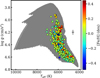 |
Fig. 1 Kiel diagram showing 779 selected planet host stars overlaid on the main-sequence model grid (grey points). The marker shows median uncertainties of 0.05 dex in log g and 60 K in Teff. |
3 The radius valley
Figure 2 (top panel) shows the planet radius distribution based on both our revised estimates and literature values from the NASA Exoplanet Archive. The revised distribution (orange line) displays a clear bimodal structure, with a valley around 2 R⊕ and peaks near −1.4 R⊕ and −2.5 R⊕. This bimodality is evident in both the histogram and the kernel density estimate, KDE (estimated by placing a Gaussian kernel at each data point and summing them to produce a continuous distribution) calculated using a bandwidth of 0.33 R⊕. For comparison, the distribution based on the literature values compiled in the NASA Exoplanet Archive is shown in black.
Our updated planetary radius measurements suggest that the radius valley is only partially populated. This aligns with the interpretation of Fulton & Petigura (2018), who argued that the valley is not entirely devoid of planets. Van Eylen et al. (2018), using a sample of 117 planets orbiting stars with precisely measured radii from asteroseismology, found the valley to be wider and more depleted. They proposed that the valley may be intrinsically empty and that the apparent infill in other studies could stem from larger radius uncertainties. Since our typical planetary radius precision is comparable due to the high level of precision of the MAISTEP stellar inputs (relative median uncertainty of −5%, see Fig. 2), their conclusion may have been influenced by the limited sample size.
The top panel of Fig. 2 also shows that our revised distribution yields a well-defined valley that is deeper than that based on literature values. The depth of the radius valley has been shown in previous studies to correlate with data quality, specifically, the reliability of planetary radii, which in turn depends critically on the host star radius (e.g. Fulton et al. 2017; Fulton & Petigura 2018; Ho & Van Eylen 2023; de Laverny et al. 2025). Our method, described in Sect. 2, provides stellar radius estimates with median precision of 2%, leading to planetary radii with a median relative uncertainty of 5%, a significant improvement over the 10% uncertainty derived from the values in the NASA Exoplanet Archive, as shown in the lower panel of Fig. 2.
To quantify the depth of the valley, Fulton et al. (2017) introduced the metric VA, defined as
 (4)
(4)
where Nvalley, Nfirst, and Nsecond represent the estimated number of planets in the valley, first peak, and second peak, respectively. In this analysis, these values were determined based on the radius ranges of 1.67-2.32 R⊕, 1.35-1.67 R⊕, and 2.32-2.8 R⊕, respectively. A value of VA = 1 corresponds to a log-uniform distribution, while lower values indicate a more pronounced valley. Using our updated radii, we find VA = 0.686, compared to VA = 0.824 based on values in the NASA Exoplanet Archive, confirming that our revised valley is deeper. In the next sections, we examine how the location of the radius valley varies with orbital and stellar parameters.
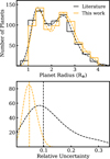 |
Fig. 2 Top panel: histograms of planet radii from the literature (black) and our revised values (orange), using 0.33 R⊕ bin width. Dashed curves represent kernel density estimates (KDEs) computed with 0.33 R⊕ bandwidth. Lower panel: KDE distributions of radius uncertainties, with vertical dashed lines indicating the medians: 0.05 (this work) and 0.10 (literature values from the NASA Exoplanet Archive). |
3.1 Orbital period dependence
Figure 3 shows the planets in our sample on a period-radius diagram, where the radius valley appears as a gap in the distribution, sloping downward towards longer orbital periods. Given that the slope of the valley carries information about the physical mechanisms responsible for shaping it, we quantified this feature using the gapfit5 tool (Loyd et al. 2020). In brief, the approach involves testing various straight-line models that describe how the valley depends on an independent parameter, such as orbital period. For each model, the predicted valley radius is computed individually for each planet based on its orbital period, and this value is subtracted from the planet’s observed (inferred) radius. This centres the valley at the zero line on the transformed radius axis, serving as the origin for measuring radius deviations. KDE is then applied to evaluate the number density of planets near the gap. The best-fit valley model is the one that minimises the planet density at zero in the transformed space. Uncertainties in the fitted gap parameters are estimated by bootstrap resampling of the observed data. Each iteration randomly samples these points with replacement, fits the gap parameters to the resampled set, and builds a distribution of fits to quantify the parameter uncertainties.
We model the valley as a linear trend in the log-log space:
![Mathematical equation: \text{log}_{10} (R_{\text{p}}) = \alpha_{\text{rv}}\times[\text{log}_{10}(P) - \text{log}_{10}(P,0)] + \text{log}_{10} (R_{\text{p,0}}),](/articles/aa/full_html/2026/03/aa57554-25/aa57554-25-eq10.png) (5)
(5)
where log10(Rp) is the planet radius, log10(P) is the orbital period, and the valley location is parameterised by the slope αrv and the intercept, log10(Rp,0). log10(P, 0) is a reference fixed orbital period, chosen near the centre of the data to minimise the correlation between slope and intercept in the fit, following Loyd et al. (2020).
The planet sample was further restricted to only those with radii between 1.4 and 2.6 R⊕, to focus the fit primarily on the distribution within the valley. The initialisation parameters were: log10(P, 0) = 1, representing the reference period in the gap line equation; an initial guess for the planet size, log10Rp,0 = 0.3; an initial slope guess of αrv = −0.15; and a width σ = 0.15 for the KDE used in the fitting. We allowed the valley line to vary within a range of ±0.5 from the initial logRp,0, and the analysis included n = 1000 bootstrap simulations with replacement using the Nelder-Mead simplex optimisation method (Nelder & Mead 1965). The sensitivity of the fits to the choice of these parameters is discussed in detail by Loyd et al. (2020). From the resulting fits, we extracted the median and the 16th and 84th percentiles to define the 68% confidence interval. The best-fit line and its uncertainty envelope, shown as an orange-shaded region below and above the line in the plot, indicate a trend in the radius valley with a slope  .
.
This slope aligns with previous observational studies (e.g. Van Eylen et al. 2018; Fulton & Petigura 2018; Martinez et al. 2019; Petigura et al. 2022; Ho & Van Eylen 2023) and has been explained by evolution models based on photoevaporation or core-powered mass loss. In photoevaporation, the mass-loss timescale for planets with small envelopes decreases during evaporation, leading to complete stripping, while it increases for larger envelopes, peaking when the planet radius roughly becomes twice the core size. As a result, some planets retain substantial envelopes that inflate their radii, while others are stripped down to bare cores. Higher core-mass planets resist evaporation, raising the transition radius at short periods. At longer periods, even low-mass planets can retain envelopes, shifting the radius valley and rocky planet sizes downwards. The predicted slopes of the valley by photoevaporation are in the range between −0.1 ≤ αrv ≤ −0.25, depending on the evaporation efficiency and the choice of model, with numerical simulations typically producing shallower trends than analytical estimates (Owen & Wu 2013, 2017).
Under core-powered mass loss, the planet’s equilibrium temperature, Tequ, determines its atmospheric cooling timescale, and the mass-loss timescale has an exponential dependence on both orbital period and planet size. As planets lose mass, they can also contract, which increases the mass-loss timescale. At some point, the two timescales match, a condition which determines whether a planet ends up above or below the valley. Since  , planets at longer orbital periods (lower Tequ) cool more slowly, allowing even small cores to retain their envelopes. Using an analytical model within this framework, Gupta & Schlichting (2019) derived a slope of −0.11.
Scenarios involving the late formation of rocky planets in gas-poor environments predict that, under the assumed radial power-law of slope −1.5 for the planetesimal disc surface density, the amount of solid material increases with distance from the star, leading to a transition radius trend with a positive sign (e.g. Lee et al. 2014; Lee & Chiang 2016; Lopez & Rice 2018; Lee 2019). Venturini et al. (2024) predicted a slope of  using a hybrid model of planet formation and photoevaporation.
Two other regions in Fig. 3 exhibit a notable scarcity of planets. First, there is a deficit of sub-Neptune-sized planets (≳2 R⊕) at very short orbital periods (≲2 days). Given that planets of this size would be readily detectable in this parameter space, the observed lack is thought to be physical rather than due to observational bias. This region of low subNeptune occurrence is referred to as the sub-Neptune desert or savanna (e.g. Szabó & Kiss 2011; Beauge & Nesvorný 2012; Lundkvist et al. 2016; West et al. 2019; Bourrier et al. 2023; Castro-González et al. 2024). Secondly, the apparent scarcity of super-Earth-sized planets at longer orbital periods is primarily attributed to reduced detection efficiency and survey completeness in this regime (see e.g. Petigura et al. 2022). At these separations, small planets produce fewer and shallower transits, making them more difficult to detect in transit surveys such as Kepler. Although the radius valley is commonly analysed using orbital period, we also explore its dependence on incident stellar flux.
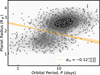 |
Fig. 3 Planet radius against orbital period. Small circles represent individual planet detections. Contours show the two-dimensional KDE of the planet population. The orange line is the best-fit trend, with a shaded band indicating the 68% confidence interval from bootstrap sampling. The error bar indicate the median uncertainty in planet radius. |
3.2 Incident flux dependence
We computed the stellar flux incident on a planet by assuming flux conservation under isotropic radiation, as described by the inverse-square law:
 (6)
(6)
where L* is the luminosity of the host star, calculated using Eq. (1), and a is the semimajor axis of the planet’s orbit. Assuming circular orbits and applying Kepler’s law, a was determined as follows:
 (7)
(7)
where P denotes the orbital period provided by the NASA Exoplanet Archive. We assumed circular orbits because only 119 planets have measured orbital eccentricities.
In Fig. 4, we present the distribution of planets on an incident flux-radius plane. Using the same fitting procedure described in Sect. 3.1, we fitted the radius valley, modifying only the initial guess for the slope and reference point in incident flux to account for the observed trend and the change in the x axis parameter. Unlike in the case with orbital period, the slope here is positive, with a value  (note that the incident flux in the horizontal axis is reverted to keep a similar distribution of the points, which explains the change of sign). This implies that the incident flux scales with the orbital period according to
  for a given host star mass (see Eqs. (6) and (7)). Such a trend has also been reported by Fulton & Petigura (2018), Martinez et al. (2019), and Ho & Van Eylen (2023). Figure 4 also shows a scarcity of sub-Neptunes at high incident flux and superEarths at low flux, as was previously discussed in the context of orbital period (Sect. 3.1). Owing to the luminosity-mass relation for main-sequence stars, we also investigate the dependence of the valley on host star mass.
3.3 Stellar mass dependence
Figure 5 shows that the valley appears at larger radius with increasing stellar mass, with a slope of  . This finding agrees with that of Berger et al. (2020a), who reported a slope of
  (our measurement has smaller errors), and is consistent within 1σ that of Ho & Van Eylen (2023),
  . Our inferred slope also aligns with predictions from photoevaporation and core-powered mass loss evolution models. In a photoevaporation model, Owen & Wu (2017) and Rogers et al. (2021) predicted slopes of 0.32 and 0.29, respectively. Wu (2019) also showed that reproducing the observed stellarmass dependence of the radius valley within a photoevaporation framework requires assuming a linear scaling between planet and host mass, proposing that the peak of the planet mass distribution scales with stellar mass as
  , with β in the range [0.95,1.40]. This implies a radius scaling of
  , where α falls between 0.23 and 0.35, encompassing our inferred slope within 1σ (
 ). Photoevaporation, driven by the total high-energy XUV radiation from stellar activity, scales as
  (Jackson et al. 2012). This would prevent close-in planets around low-mass stars from retaining their envelopes. Therefore, subNeptunes around these stars are mostly found on wide orbits, while closer-in planets are stripped down to rocky cores.
Gupta & Schlichting (2020) in a core-powered mass-loss model, predicts a slope of ~0.35 based on numerical simulations, and a slightly shallower slope of ~0.33 from analytical estimates, assuming a fixed period distribution and employing the bolometric luminosity-mass relation. The similarity in the predicted slopes of both models suggests that our measured slope of  does not favour one model over the other. In a hybrid model of formation and photoevaporation by Venturini et al. (2024), which considers an extended stellar mass range of 0.1-1.5 M⊙, a shallow slope of
  was predicted.
Another feature, evident from the KDE contours in Fig. 5, is the systematic shift in the peaks of both planetary populations on either side of the valley towards larger radii with increasing stellar mass. We quantify this trend by classifying the sample into super-Earths and sub-Neptunes using a radius split at 1.98 R⊕, which is the derived centroid of the valley in one-dimension determined using a Gaussian model mixture (GMM) grouping (see also Fig. 2). We performed bootstrap linear regression within each group to derive power-law relations between planet radius and stellar mass, as shown in blue and purple in Fig. 5. We find slopes of  for sub-Neptunes and
  for super-Earths, respectively. The steeper slope for sub-Neptunes indicates a stronger dependence of planet size on stellar mass for this sample compared to super-Earths. The difference in slopes may suggest that higher-mass stars slightly inflate the radii of their planets, leading to a steeper slope in the sub-Neptune population, but not in the bare, rocky super-Earths. Generally, these results highlight that planets orbiting stars in our study mass range (0.7-1.6 M⊙) tend to be systematically larger around more massive stars, with the radius valley location changing to larger planets as stellar mass increases. This trend likely reflects the dependence of core size growth on the amount of solid material in the protoplanetary disc, which scales with stellar mass (e.g. Andrews et al. 2013; Pascucci et al. 2016; Ansdell et al. 2017). Consequently, this scaling influences not only planets within the valley, but also those on either side encompassing rocky super-Earths and gaseous sub-Neptunes (e.g. Wu 2019).
A similar trend is visible in the figures of Fulton & Petigura (2018, Fig. 8) and Berger et al. (2020a, Fig. 5), both showing a positive RP-M* correlation for sub-Neptunes, super-Earths, and the valley population across stellar mass ranges of roughly 0.81.3 M⊙ and 0.5-1.5 M⊙, respectively, although the trend was not quantified statistically. In a core-powered mass-loss scenario, Gupta & Schlichting (2020) attribute the observed trend in both the radius valley and the two populations to the assumption that the orbital period distribution is assumed to be independent of stellar mass (motivated by observation data in Fulton & Petigura 2018). As a result, planets at the same orbital period will have higher Tequ around more massive (i.e. more luminous) stars. For a constant orbital period,  , with α being the power-law index in the stellar mass-luminosity relation. The higher Tequ enhances the atmospheric escape, pushing the radius valley to larger sizes and shifting both the sub-Neptunes and super-Earths to higher Tequ regions.
Petigura et al. (2022) applied a 1.7 R⊕ radius cut to planets orbiting stars in the 0.5-1.4 M⊙ range and reported a stellar mass dependence for sub-Neptunes, with a slope of  , consistent within 1σ with our estimate of
  . They did not find a comparable trend for super-Earths, reporting a much shallower slope of
  , which is notably lower than the values we derive. This slope is also lower compared the apparent trend in Fulton et al. (2017), Berger et al. (2020a) and the inference of 0.23-0.35 from Wu (2019). Petigura et al. (2022) suggested that more massive protoplanetary discs around higher-mass stars allow sub-Neptune cores to accrete thicker gaseous envelopes, resulting in larger observed radii. These cores grow roughly linearly with stellar mass, following
  , and can exceed the threshold mass above which atmospheric stripping becomes inefficient. As a result, many sub-Neptune planets retain substantial envelopes despite ongoing loss processes. In contrast, super-Earths are likely stripped cores that fall below this threshold. Because the radii of rocky planets increase only weakly with core mass, their sizes remain nearly constant across a range of host masses. Therefore, the apparent increase in planet size with stellar mass for super-Earths in Fig. 5 may result from the slightly higher masses for a subset of stars in this work compared to values reported in the literature (see Fig. A.1).
The main-sequence lifetime of a star depends strongly on its mass, approximately following τms ~ 10 Gyr (M*/M⊙)−2.5 (Kippenhahn et al. 1990, 2012). This mass-age correlation implies that the radius valley may also depend on the age of the star-planet system. In the following section, we use stellar age estimates from MAISTEP to investigate the temporal evolution of features in the small-sized exoplanet population.
3.4 Stellar age dependence
The age of a planetary system is typically inferred from that of its host star, as planets form during the early stages of stellar evolution (Meyer 2008). However, stellar age is not directly observable and remains one of the most difficult stellar parameters to determine, especially for field stars, with no single method performing reliably across all stellar types and evolutionary stages. Asteroseismology provides highly precise stellar age estimates, but the number of main-sequence stars with seismic detections and confirmed exoplanets remains <100 (Silva Aguirre et al. 2015; Campante et al. 2015; Lundkvist et al. 2016; Lund et al. 2017; Campante et al. 2019). This is expected to change with the upcoming ESA’s PLATO mission (Rauer et al. 2014).
In Kamulali et al. (2025), we assessed stellar age estimates from MAISTEP, derived using only atmospheric constraints, by comparing them to asteroseismic ages for a sample of Kepler legacy main-sequence stars. The MAISTEP stellar ages relative to the asteroseismic ages showed a bias of 7%, a scatter of 23%, and an average fractional uncertainty of 28%. Using the same methodology, we estimated the ages of host stars in this study, achieving an average fractional uncertainty of 23%. To minimise the impact of poorly constrained ages, we excluded 46 host stars with flat age distributions, resulting in a final sample of 823 planets orbiting 718 unique hosts. The removed stars typically have median ages near the grid midpoint (~7 Gyr) with broad uncertainties (στ ≳ 3.5 Gyr). They are low-mass (≲1.0 M⊕), and have Teff ≲ 5600 K. Given their small number, excluding these objects has a minor impact on observed mass and age trends.
Figure 6 presents the distribution of planet radii as a function of stellar age. The radius valley shows minimal variation with age, and a power-law fit to its location yields a slope of  , indicating no significant age dependence. Using isochrone-based ages, Ho & Van Eylen (2023) similarly reported a shallow slope of
  .
.
The variation in the average sizes of planet populations above and below the radius valley with age was also examined. The resulting fits, shown in blue and purple in Figure 6, with slopes of  and
and  for sub-Neptunes and super-Earths, respectively, reveals no significant dependence.
These findings are consistent with those of Petigura et al. (2022) based on isochrone ages. In contrast, Chen et al. (2022), employing a kinematic method based on the average agevelocity dispersion relation for the LAMOST-Gaia-Kepler sample, reported a decline in average sub-Neptune size with increasing age, which is consistent with theoretical expectations. Both photoevaporation and core-powered mass loss models predict a decrease in sub-Neptune size over time with a slope of −0.1, while super-Earth sizes are expected to remain largely constant. The discrepancy between these predictions and the findings based on our age estimates or isochrones may reflect limitations in stellar age determinations, underscoring the need for followup analysis using asteroseismic ages when they become available for a wider sample of host stars.
An alternative approach to probing the time evolution of close-in exoplanets is to examine the ratio of super-Earths to sub-Neptunes, which we denote as NE/NN. As sub-Neptunes are thought to lose their atmospheres over time and evolve into super-Earths, this ratio offers a population-level tracer of evolutionary processes. In this context, an increasing NE/NN with system age may reflect the cumulative effects of atmospheric erosion over time, providing a complementary perspective to more direct observational signatures such as the radius valley or individual mass-radius measurements.
We estimated the ratios by dividing the planetary sample into two age bins: systems younger than 3 Gyr and those older than 3 Gyr. We used 3 Gyr as the dividing point, as only ten planets in our sample are hosted by stars with median ages below 1 Gyr. A GMM was applied to identify the location of the radius valley in one dimension, after which we computed the number of planets below (super-Earths, NE) and above (sub-Neptunes, NN) the valley. The observational data were resampled 1000 times with replacement to estimated the uncertainties in NE/NN. This approach yielded  for the younger systems and
  for the older systems, as shown in the top panel of Fig. 7. Additionally, the radius valley in the older population appears shallower and shifted to larger radii compared to the younger sample, based on the positions of the GMM-derived minima. The shift towards larger radii may reflect cumulative atmospheric loss in sub-Neptunes occurring over gigayear timescales. However, the large number of planets in the old sample (687 compared to 136 in the young population) may lead to a statistically biased result.
To examine potential sample size effects while accounting for age-related degeneracies, we selected a subset of older systems whose host metallicity, radius, and mass distributions closely resemble those of the younger population, with ages below 3 Gyr. We employed optimal transport (OT: Flamary et al. 2021, 2024) in Python to identify a minimal-cost mapping between the joint distributions of stellar metallicity, radius, and mass for the two groups. Using the OT cost matrix, we computed a one-to-one assignment via the Hungarian algorithm (Kuhn 1955), yielding an old-star subset whose multivariate distribution closely reproduces that of the young sample. The Kolmogorov-Smirnov tests on the distributions of stellar metal-licity, radius, and mass returned p-values of 0.95, 0.24, and 0.02, respectively, indicating that the young and old samples are statistically consistent in stellar metallicity and radius, with some differences in mass. As shown in the bottom panel of Fig. 7, the resulting ratio for the matched older sample is  , which is consistent within uncertainties with the value of
  derived for the full older population. Therefore, at older ages, we find a higher prevalence of super-Earths relative to sub-Neptunes, suggesting that some sub-Neptunes evolve into super-Earths over time.
The change in the NE/NN ratio was first reported by Berger et al. (2020a), who used isochrone-based ages. They found that the ratio increased from 0.61 ± 0.09 for systems younger than 1 Gyr to 1.00 ± 0.10 for those older than 1 Gyr, focusing on hotter stars (5700-7900 K). A separate study by Sandoval et al. (2021), which included cooler GK-type stars (Teff < 5800 K), explored age divisions at both 1 Gyr and 3 Gyr. Using the 3 Gyr cut, they reported NE/NN = 0.78 ± 0.17 for younger systems and 1.00 ± 0.04 for older ones. Our results exhibit a similar age-dependent trend in NE/NN, albeit with somewhat lower absolute values. As observed in David et al. (2021) and Ho & Van Eylen (2023), we also find that the radius valley shifts to higher planetary radii and becomes shallower, indicating that the valley evolves over time. David et al. (2021) suggested that the positive age trend arises from the scarcity of large super-Earths (~1.5-1.8 R⊕) orbiting young stars, a feature also evident in our Fig. 7.
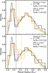 |
Fig. 7 Radius distributions of young (black) and old (orange) planets. Top: full population. Bottom: property-matched sample in stellar metal-licity, radius, and mass using optimal transport. Vertical dashed lines show the centroid of the inferred radius gap from GMM fits. Sample sizes, N, and ratios, NE/NN, are indicated in panel legends. |
3.5 Four-dimensional radius valley
A multidimensional radius valley has been proposed to better separate photoevaporation from core-powered mass loss. Here, we model the radius valley as a four-dimensional plane in the parameter space of planetary radius, orbital period, stellar mass, and stellar age following the expression
 (8)
(8)
where α, β, γ, are the coefficients (power-law indices) in orbital period, stellar mass, and age, respectively, and δ is the intercept on the planet radius axis.
To achieve this, we used the logistic regression model implemented in Python via the scikit - learn package. Unlike the gapfit method (see Sect. 3.1), which is limited to two dimensions, logistic regression can be directly extended to higher dimensions. Logistic regression models the probability of a binary outcome from one or more predictor variables. We first separated the sample into two groups, those above and below the valley, on the radius-orbital period-mass-age plane, using a two-component GMM. We identified the sub-Neptune (sN) and super-Earth (sE) classes by comparing the mean log10(RP) of the two components; the cluster with the larger mean radius is taken as the sN population. To select an optimal regularisation parameter C for logistic regression, we performed a five-fold cross-validation with GMM embedded in each fold to classify planets as sN or sE based on their radii distribution. Candidate C values spanning 1-1000 were tested, and C = 50 maximised the mean classification accuracy across folds, and was used in the final model. Bootstrapping with 1000 resamples of the 823 planets (with replacement) was performed to estimate the uncertainties in the coefficients. The posterior distributions of all coefficients are summarised using the median and the 16th- 84th percentile ranges.
We find coefficients of  ,
,  , and
, and  , and an intercept of
  . In Fig. 8, we present a three-dimensional visualisation of the radius valley in the space of planet radius, orbital period, and stellar mass, with points colour-coded according to stellar age. The derived coefficients in four-dimensional fit are consistent with the corresponding slopes in two dimensions based on the gapfit method (
 in orbital period,
  in stellar mass, and
  in stellar age). They are also consistent with the four-dimensional coefficients reported by Ho & Van Eylen (2023), derived from a linear support vector machine fit to orbital period, stellar mass, and stellar age. The slightly higher stellar age slope in our analysis,
  versus their
  (Ho & Van Eylen 2023), likely reflects differences in stellar age estimates arising from variations in the underlying physics of the stellar models (see Fig. A.2.)
Our four-dimensional radius valley provides strong support for core-powered mass-loss models, as the evolution unfolds on gigayear timescales (Ginzburg et al. 2016, 2018; Gupta & Schlichting 2019, 2020). On the other hand, photoevaporation is predicted to be most effective within the first ~100 Myr when high-energy output from Sun-like stars peaks (e.g. Jackson et al. 2012; Tu et al. 2015), although some fraction of subNeptunes are predicted to transform to super-Earths on longer timescales (Rogers et al. 2021). Moreover, King & Wheatley (2021) found that UV radiation remains substantial beyond 100 Myr, suggesting that the process may extend longer than previously thought. We also note, however, that age trends remain inconclusive because of substantial uncertainties in stellar age estimates; accordingly, these interpretations should be regarded with caution.
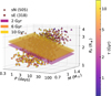 |
Fig. 8 Four-dimensional exoplanet radius valley across orbital period, stellar mass, and age space. Observed planets are overlaid, coloured by age, with sub-Neptunes (sNs) and super-Earths (sEs) distinguished by marker type. The fitted planes show the valley at representative ages of 2, 6, and 10 Gyr. |
4 Summary and conclusions
In this study, we analysed a sample of 779 stars from the SWEET-Cat database, hosting 893 confirmed planets listed in the NASA Exoplanet Archive, to revisit the size distribution of small, close-in exoplanets. Our primary focus was to re-examine the existence and depth of the radius valley, and how its location varies with orbital period, incident flux, stellar mass, and stellar age. We derived stellar radii, masses, and ages using MAISTEP, a grid-based machine-learning stellar parameter estimator, achieving median fractional uncertainties of 2, 2, and 27%, respectively, using only effective temperatures and metal-licities from spectroscopy, along with Gaia -based luminosities. We note that we are able to achieve the radius and mass precision typically expected when asteroseismic data are available. Planetary radii were updated accordingly, reaching a median fractional uncertainty of 4%.
Our revised planet radii reveal a well-defined bimodal distribution, with peaks near ~1.5 R⊕ (super-Earths) and ~2.6 R⊕ (sub-Neptunes), separated by a valley around 2 R⊕, consistent with previous studies. We find that the radius valley is partially filled and deeper than in the distribution based on the planetary radii in the NASA Exoplanet Archive (Fig. 2).
The location of the valley shifts toward smaller radii at longer orbital periods (i.e. lower incident flux), yielding a power-law slope of  when modelled in terms of orbital period, or equivalently
  with respect to incident flux (Figs. 3 and 4, respectively). The average size of planets within the radius valley increases with host star’s mass, with a slope of
  . The characteristic sizes of sub-Neptunes and super Earths show trends with slopes of
  and
and  , respectively, indicating a stronger dependence in sub-Neptunes than in super-Earths (Fig. 5).
Regarding stellar age, we find that the ratio of super-Earths to sub-Neptunes increases from  in systems younger than 3 Gyr to
  in older systems (Fig. 7). The radius valley also becomes shallower and shifts to larger radii in the older systems, confirming age-dependent evolution in planet demographics over gigayear timescales. A four-dimensional (planetary radius, orbital period, stellar mass, and stellar age) characterisation of the valley yields slopes in orbital period and mass similar to those in two dimensions (planet radius-orbital period and planet radius-stellar mass), and a slope of
  in stellar age. The observed gigayear-scale trends are consistent with corepowered mass loss as an important driver of atmospheric escape, although photoevaporation cannot be fully ruled out, given theoretical expectations that it may continue to operate on timescales exceeding ~100 Myr.
Finally, the average size of sub-Neptunes does not show a decline with time. This lack of an observed decline may stem from the large uncertainties in our host age estimates, despite theoretical expectations that sub-Neptunes gradually shrink and evolve into super-Earths. These findings underscore the need for more precise host star age measurements, which future asteroseismic observations, such as those expected from ESA’s PLATO mission (Rauer et al. 2014), are likely to provide.
Acknowledgements
We thank the referee for the insightful suggestions that improved the manuscript. J.K. acknowledges funding through the Max-Planck Partnership group - SEISMIC between Max-Planck-Institut für Astrophysik (MPA) - Germany and Kyambogo University (KyU) - Uganda. B.N. and O.T. acknowledge funding through the Max Planck - Humboldt research unit established in Uganda at Kyambogo University. B.N. also acknowledges funding from the UNESCO-TWAS programme, “Seed Grant for African Principal Investigators” financed by the German Ministry of Education and Research (BMBF). T.L.C is supported by Fundação para a Ciência e a Tecnologia (FCT) in the form of a work contract (2023.08117.CEECIND/CP2839/CT0004). S.G.S acknowledges the support from FCT through Investigador FCT contract nr. CEECIND/00826/2018 and POPH/FSE (EC). N.M. acknowledges the research theory grant “Synergic tools for characterizing solar-like stars and habitability conditions of exoplanets” under the INAF national call for Fundamental Research 2023. V.A. and N.C.S. acknowledge support from FCT - Fundação para a Ciência e Tecnologia through national funds and from FEDER via COMPETE2020 - Programa Operacional Competitividade e Internacionaliza-ção, under the grants UIDB/04434/2020 (DOI: 10.54499/UIDB/04434/2020) and UIDP/04434/2020 (DOI: 10.54499/UIDP/04434/2020). V.A. is also supported through a work contract funded by the FCT Scientific Employment Stimulus program (reference 2023.06055.CEECIND/CP2839/CT0005, DOI: 10.54499/2023.06055.CEECIND/CP2839/CT0005). Views and opinions expressed are however those of the author(s) only and do not necessarily reflect those of the European Union or the European Research Council. Neither the European Union nor the granting authority can be held responsible for them. Software : Data analysis in this manuscript was carried out using the Python 3.10.12 libraries; scikit-learn 1.5.1 (Pedregosa et al. 2011), pandas 2.2.2 (McKinney et al. 2010), NumPy 1.26.4 (Van Der Walt et al. 2011), and SciPy 1.14.1 (Virtanen et al. 2020).
References
- Akeson, R. L., Chen, X., Ciardi, D., et al. 2013, PASP, 125, 989 [Google Scholar]
- Andrae, R., Fouesneau, M., Creevey, O., et al. 2018, A&A, 616, A8 [NASA ADS] [CrossRef] [EDP Sciences] [Google Scholar]
- Andrews, S. M., Rosenfeld, K. A., Kraus, A. L., & Wilner, D. J. 2013, ApJ, 771, 129 [Google Scholar]
- Angulo, C., Arnould, M., Rayet, M., et al. 1999, Nucl. Phys. A, 656, 3 [Google Scholar]
- Ansdell, M., Williams, J. P., Manara, C. F., et al. 2017, AJ, 153, 240 [Google Scholar]
- Asplund, M., Grevesse, N., Sauval, A. J., & Scott, P. 2009, ARA&A, 47, 481 [CrossRef] [Google Scholar]
- Astraatmadja, T. L., & Bailer-Jones, C. A. 2016, ApJ, 833, 119 [NASA ADS] [CrossRef] [Google Scholar]
- Beauge, C., & Nesvorny, D. 2012, ApJ, 763, 12 [Google Scholar]
- Berger, T. A., Huber, D., Gaidos, E., van Saders, J. L., & Weiss, L. M. 2020a, AJ, 160, 108 [NASA ADS] [CrossRef] [Google Scholar]
- Berger, T. A., Huber, D., Van Saders, J. L., et al. 2020b, AJ, 159, 280 [Google Scholar]
- Berger, T. A., Schlieder, J. E., & Huber, D. 2023a, arXiv e-prints [arXiv:2301.11338] [Google Scholar]
- Berger, T. A., Schlieder, J. E., Huber, D., & Barclay, T. 2023b, arXiv e-prints [arXiv:2302.00009] [Google Scholar]
- Borucki, W. J., Koch, D., Basri, G., et al. 2010, Science, 327, 977 [Google Scholar]
- Bourrier, V., Attia, M., Mallonn, M., et al. 2023, A&A, 669, A63 [NASA ADS] [CrossRef] [EDP Sciences] [Google Scholar]
- Breiman, L. 2001, Mach. Learn., 45, 5 [Google Scholar]
- Burn, R., Bali, K., Dorn, C., Luque, R., & Grimm, S. L. 2024a, arXiv e-prints [arXiv:2411.16879] [Google Scholar]
- Burn, R., Mordasini, C., Mishra, L., et al. 2024b, Nat. Astron., 8, 463 [Google Scholar]
- Campante, T. L., Barclay, T., Swift, J. J., et al. 2015, ApJ, 799, 170 [Google Scholar]
- Campante, T. L., Corsaro, E., Lund, M. N., et al. 2019, ApJ, 885, 31 [Google Scholar]
- Casagrande, L., & VandenBerg, D. A. 2018, MNRAS, 479, L102 [NASA ADS] [CrossRef] [Google Scholar]
- Castro-González, A., Bourrier, V., Lillo-Box, J., et al. 2024, A&A, 689, A250 [NASA ADS] [CrossRef] [EDP Sciences] [Google Scholar]
- Chakrabarty, A., & Mulders, G. D. 2024, ApJ, 966, 185 [Google Scholar]
- Chen, T., & Guestrin, C. 2016, in Proceedings of the 22nd acm sigkdd international conference on knowledge discovery and data mining, 785 [Google Scholar]
- Chen, D.-C., Xie, J.-W., Zhou, J.-L., et al. 2022, AJ, 163, 249 [NASA ADS] [CrossRef] [Google Scholar]
- Choi, J., Dotter, A., Conroy, C., et al. 2016, ApJ, 823, 102 [Google Scholar]
- Cloutier, R., & Menou, K. 2020, AJ, 159, 211 [NASA ADS] [CrossRef] [Google Scholar]
- Cox, J. P., & Giuli, R. T. 1968, Principles of Stellar Structure: Physical Principles (New York: Gordon and Breach), 1 [Google Scholar]
- David, T. J., Contardo, G., Sandoval, A., et al. 2021, AJ, 161, 265 [NASA ADS] [CrossRef] [Google Scholar]
- deLaverny, P., Ligi, R., Crida, A., Recio-Blanco, A., & Palicio, P. A. 2025, A&A, 699, A100 [Google Scholar]
- Dotter, A. 2016, ApJS, 222, 8 [Google Scholar]
- Ferguson, J. W., Alexander, D. R., Allard, F., et al. 2005, ApJ, 623, 585 [Google Scholar]
- Flamary, R., Courty, N., Gramfort, A., et al. 2021, J. Mach. Learn. Res., 22, 1 [Google Scholar]
- Flamary, R., Vincent-Cuaz, C., Courty, N., et al. 2024, POT Python Optimal Transport (version 0.9.5) [Google Scholar]
- Fulton, B. J., & Petigura, E. A. 2018, AJ, 156, 264 [Google Scholar]
- Fulton, B. J., Petigura, E. A., Howard, A. W., et al. 2017, AJ, 154, 109 [Google Scholar]
- Gaia Collaboration (Vallenari, A., et al.) 2023, A&A, 674, A1 [NASA ADS] [CrossRef] [EDP Sciences] [Google Scholar]
- Ginzburg, S., Schlichting, H. E., & Sari, R. 2016, ApJ, 825, 29 [Google Scholar]
- Ginzburg, S., Schlichting, H. E., & Sari, R. 2018, MNRAS, 476, 759 [Google Scholar]
- Green, G. 2018, J. Open Source Softw., 3, 695 [NASA ADS] [CrossRef] [Google Scholar]
- Gupta, A., & Schlichting, H. E. 2019, MNRAS, 487, 24 [Google Scholar]
- Gupta, A., & Schlichting, H. E. 2020, MNRAS, 493, 792 [Google Scholar]
- Herwig, F. 2000, arXiv e-prints [arXiv:astro-ph/0007139] [Google Scholar]
- Ho, C. S., & Van Eylen, V. 2023, MNRAS, 519, 4056 [NASA ADS] [CrossRef] [Google Scholar]
- Huber, D., Aguirre, V. S., Matthews, J. M., et al. 2014, ApJS, 211, 2 [NASA ADS] [CrossRef] [Google Scholar]
- Huber, D., Zinn, J., Bojsen-Hansen, M., et al. 2017, ApJ, 844, 102 [Google Scholar]
- Iglesias, C. A., & Rogers, F. J. 1996, ApJ, 464, 943 [NASA ADS] [CrossRef] [Google Scholar]
- Imbriani, G., Costantini, H., Formicola, A., et al. 2005, Eur. Phys. J. A-Hadrons Nuclei, 25, 455 [Google Scholar]
- Jackson, A. P., Davis, T. A., & Wheatley, P. J. 2012, MNRAS, 422, 2024 [Google Scholar]
- Johnson, J. A., Petigura, E. A., Fulton, B. J., et al. 2017, AJ, 154, 108 [Google Scholar]
- Kamulali, J., Nsamba, B., Adibekyan, V., et al. 2025, A&A, 695, A57 [NASA ADS] [CrossRef] [EDP Sciences] [Google Scholar]
- King, G. W., & Wheatley, P. J. 2021, MNRAS, 501, L28 [Google Scholar]
- Kippenhahn, R., Weigert, A., & Weiss, A. 1990, Stellar Structure and Evolution (Berlin: Springer), 192 [Google Scholar]
- Kippenhahn, R., Weigert, A., & Weiss, A. 2012, Stellar Structure and Evolution (Berlin Heidelberg: Springer-Verlag) [Google Scholar]
- Krishna Swamy, K. 1966, ApJ, 145, 174 [CrossRef] [Google Scholar]
- Kuhn, H. W. 1955, Naval Res. Logistics Quarterly, 2, 83 [Google Scholar]
- Kunz, R., Fey, M., Jaeger, M., et al. 2002, ApJ, 567, 643 [CrossRef] [Google Scholar]
- Lebreton, Y., & Reese, D. R. 2020, A&A, 642, A88 [NASA ADS] [CrossRef] [EDP Sciences] [Google Scholar]
- Lee, J.-E. 2019, Bull. Korean Astron. Soc., 44, 33 [Google Scholar]
- Lee, E. J., & Chiang, E. 2016, ApJ, 817, 90 [Google Scholar]
- Lee, E. J., Chiang, E., & Ormel, C. W. 2014, ApJ, 797, 95 [Google Scholar]
- Lindegren, L., Hernández, J., Bombrun, A., et al. 2018, A&A, 616, A2 [NASA ADS] [CrossRef] [EDP Sciences] [Google Scholar]
- Lindegren, L., Bastian, U., Biermann, M., et al. 2021, A&A, 649, A4 [EDP Sciences] [Google Scholar]
- Liu, S.-F., Hori, Y., Lin, D., & Asphaug, E. 2015, ApJ, 812, 164 [CrossRef] [Google Scholar]
- Lopez, E. D., & Fortney, J. J. 2013, ApJ, 776, 2 [Google Scholar]
- Lopez, E. D., & Rice, K. 2018, MNRAS, 479, 5303 [NASA ADS] [CrossRef] [Google Scholar]
- Loyd, R. P., Shkolnik, E. L., Schneider, A. C., et al. 2020, ApJ, 890, 23 [NASA ADS] [CrossRef] [Google Scholar]
- Lund, M. N., Aguirre, V. S., Davies, G. R., et al. 2017, ApJ, 835, 172 [Google Scholar]
- Lundkvist, M., Kjeldsen, H., Albrecht, S., et al. 2016, Nat. Commun., 7, 11201 [NASA ADS] [CrossRef] [Google Scholar]
- Mamajek, E. E., Torres, G., Prsa, A., et al. 2015, arXiv e-prints [arXiv:1510.06262] [Google Scholar]
- Martinez, C. F., Cunha, K., Ghezzi, L., & Smith, V. V. 2019, ApJ, 875, 29 [Google Scholar]
- Mayor, M., Marmier, M., Lovis, C., et al. 2011, arXiv e-prints [arXiv:1109.2497] [Google Scholar]
- McKinney, W., van der Walt, S., & Millman, J. 2010, Proceedings of the 9th Python in Science Conference [Google Scholar]
- Meyer, M. R. 2008, Proc. Int. Astron. Union, 4, 111 [Google Scholar]
- Moedas, N., Deal, M., Bossini, D., & Campilho, B. 2022, A&A, 666, A43 [NASA ADS] [CrossRef] [EDP Sciences] [Google Scholar]
- Moedas, N., Bossini, D., Deal, M., & Cunha, M. S. 2024, A&A, 684, A113 [NASA ADS] [CrossRef] [EDP Sciences] [Google Scholar]
- Neilson, H. R., Lester, J. B., & Baron, F. 2022, A&A, 662, A38 [NASA ADS] [CrossRef] [EDP Sciences] [Google Scholar]
- Nelder, J. A., & Mead, R. 1965, Comp. J., 7, 308 [CrossRef] [Google Scholar]
- Ogihara, M., & Hori, Y. 2020, ApJ, 892, 124 [Google Scholar]
- Owen, J. E., & Wu, Y. 2013, ApJ, 775, 105 [Google Scholar]
- Owen, J. E., & Wu, Y. 2017, ApJ, 847, 29 [Google Scholar]
- Pascucci, I., Testi, L., Herczeg, G. J., et al. 2016, ApJ, 831, 125 [Google Scholar]
- Pedregosa, F., Varoquaux, G., Gramfort, A., et al. 2011, J. Mach. Learn. Res., 12, 2825 [Google Scholar]
- Pepe, F., Cristiani, S., Rebolo, R., et al. 2021, A&A, 645, A96 [NASA ADS] [CrossRef] [EDP Sciences] [Google Scholar]
- Petigura, E. A. 2020, AJ, 160, 89 [NASA ADS] [CrossRef] [Google Scholar]
- Petigura, E. A., Howard, A. W., Marcy, G. W., et al. 2017, AJ, 154, 107 [NASA ADS] [CrossRef] [Google Scholar]
- Petigura, E. A., Rogers, J. G., Isaacson, H., et al. 2022, AJ, 163, 179 [NASA ADS] [CrossRef] [Google Scholar]
- Pijpers, F. P. 2003, A&A, 400, 241 [NASA ADS] [CrossRef] [EDP Sciences] [Google Scholar]
- Prokhorenkova, L., Gusev, G., Vorobev, A., Dorogush, A. V., & Gulin, A. 2018, Advances in neural information processing systems, 31 [Google Scholar]
- Rauer, H., Catala, C., Aerts, C., et al. 2014, Exp. Astron., 38, 249 [Google Scholar]
- Ricker, G. R., Winn, J. N., Vanderspek, R., et al. 2015, J. Astron. Teles. Instrum. Syst., 1, 014003 [Google Scholar]
- Rogers, F., & Nayfonov, A. 2002, ApJ, 576, 1064 [NASA ADS] [CrossRef] [Google Scholar]
- Rogers, J. G., Gupta, A., Owen, J. E., & Schlichting, H. E. 2021, MNRAS, 508, 5886 [NASA ADS] [CrossRef] [Google Scholar]
- Sandoval, A., Contardo, G., & David, T. J. 2021, ApJ, 911, 117 [CrossRef] [Google Scholar]
- Santos, N., Sousa, S., Mortier, A., et al. 2013, A&A, 556, A150 [NASA ADS] [CrossRef] [EDP Sciences] [Google Scholar]
- Schlichting, H. E., Sari, R., & Yalinewich, A. 2015, Icarus, 247, 81 [NASA ADS] [CrossRef] [Google Scholar]
- Silva Aguirre, V., Davies, G., Basu, S., et al. 2015, MNRAS, 452, 2127 [NASA ADS] [CrossRef] [Google Scholar]
- Skrutskie, M. F., Cutri, R., Stiening, R., et al. 2006, AJ, 131, 1163 [NASA ADS] [CrossRef] [Google Scholar]
- Sousa, S., Adibekyan, V., Delgado-Mena, E., et al. 2021, A&A, 656, A53 [NASA ADS] [CrossRef] [EDP Sciences] [Google Scholar]
- Sousa, S., Adibekyan, V., Delgado-Mena, E., et al. 2024, A&A, 691, A53 [NASA ADS] [CrossRef] [EDP Sciences] [Google Scholar]
- Szabó, G. M., & Kiss, L. 2011, ApJ, 727, L44 [CrossRef] [Google Scholar]
- Thoul, A. A., Bahcall, J. N., & Loeb, A. 1994, ApJ, 421, 828 [Google Scholar]
- Tu, L., Johnstone, C. P., Güdel, M., & Lammer, H. 2015, A&A, 577, L3 [NASA ADS] [CrossRef] [EDP Sciences] [Google Scholar]
- Van Der Walt, S., Colbert, S. C., & Varoquaux, G. 2011, Comput. Sci. Eng., 13, 22 [Google Scholar]
- Van Eylen, V., Agentoft, C., Lundkvist, M. S., et al. 2018, MNRAS, 479, 4786 [Google Scholar]
- Van Eylen, V., Astudillo-Defru, N., Bonfils, X., et al. 2021, MNRAS, 507, 2154 [NASA ADS] [Google Scholar]
- Venturini, J., Guilera, O. M., Haldemann, J., Ronco, M. P., & Mordasini, C. 2020a, A&A, 643, L1 [NASA ADS] [CrossRef] [EDP Sciences] [Google Scholar]
- Venturini, J., Guilera, O. M., Ronco, M. P., & Mordasini, C. 2020b, A&A, 644, A174 [NASA ADS] [CrossRef] [EDP Sciences] [Google Scholar]
- Venturini, J., Ronco, M. P., Guilera, O. M., et al. 2024, A&A, 686, L9 [NASA ADS] [CrossRef] [EDP Sciences] [Google Scholar]
- Virtanen, P., Gommers, R., Oliphant, T. E., et al. 2020, Nat. Methods, 17, 261 [Google Scholar]
- Wehenkel, L., Ernst, D., & Geurts, P. 2006, in Robust Methods for Power System State Estimation and Load Forecasting [Google Scholar]
- West, R. G., Gillen, E., Bayliss, D., et al. 2019, MNRAS, 486, 5094 [Google Scholar]
- Wu, Y. 2019, ApJ, 874, 91 [NASA ADS] [CrossRef] [Google Scholar]
Appendix A Comparison of stellar parameters
Exploration of the radius valley demographics is critical to the accuracy and precision of the stellar radius, mass, and age. In Kamulali et al. (2025), the stellar parameters inferred from MAISTEP were validated. Here, we compare MAISTEP-inferred parameters with the literature values for the subset of stars in common. First, we compare stellar parameters from MAISTEP for 1,221 stars to those derived using a Bayesian and Markov Chain Monte Carlo-based tool, Systematic Inference on a Massive Scale (SPInS; Lebreton & Reese 2020). Both methods incorporate the same observational constraints: Teff, [Fe/H], and L, and rely on the same grid of stellar evolutionary models. We find excellent agreement in the inferred radius, with a median offset of 0.3% and a scatter of 1.1%. The median fractional uncertainty from both methods is 2%. For stellar mass, we obtain a median offset of 0.2% and a scatter of 2.6%. The fractional uncertainties are 2% for MAISTEP and 7% for SPInS. The offset and scatter in stellar ages are 0.6% and 13.1%, respectively. We observe higher age estimates for some stars with SPInS-inferred ages between 6 and 11 Gyr. The fractional uncertainty in ages is 27% for MAISTEP, roughly half of the 47% recorded from SPInS. The observed differences in uncertainties may reflect the distinct ways the two routines handle uncertainties in the input parameters.
Next, we compare with the homogeneous estimates of Fulton & Petigura (2018) for an overlapping sample of 226 stars, shown in Fig. A.2. We note that this sample has uniform spectroscopic constraints from Petigura et al. (2017), which were used as input for the stellar parameter determinations in Fulton & Petigura (2018). Consequently, nearly all MAISTEP inferences for this subset rely on the same uniform spectroscopic dataset, ensuring consistency with Fulton & Petigura (2018). The radii, masses, and ages from MAISTEP are systematically higher by 3.9%, 1.7%, and 9.3%, with scatters of 4.4%, 5.8%, and 90%. The offsets arise partly from the fixed parallax zero-point correction of −0.053 adopted in Fulton & Petigura (2018) for the Gaia DR2 data, which impacts distance estimates and consequently the luminosity values. As discussed in the main text, we use Gaia DR3 parallaxes and G band magnitudes, with zeropoint parallax corrections that depend on the star’s magnitude, colour, and position (Lindegren et al. 2021). Our derived zeropoint correction have a median value of −0.027 mas, about half of −0.053 mas. Adopting a fixed −0.053 mas in our luminosity calculations reduces the offsets to 2% in radius, 1.1% in mass, and 4.4% in age (Fig. A.3). For a small subset of stars, slightly higher masses are apparent, a feature seen in MAISTEP mass predictions in comparison to those from SPInS (Fig. A.1). In addition, the stellar parameters in Fulton & Petigura (2018) were derived based on the MESA Isochrones and Stellar Tracks (Choi et al. 2016; Dotter 2016) via isoclassify (Huber et al. 2017), a Bayesian stellar pipeline, incorporating spectroscopic Teff and [Fe/H] from (Petigura et al. 2017), along with Gaia DR2 parallaxes and 2MASS K-band photometry (Skrutskie et al. 2006). In isoclassify, distances are inferred from parallax using a Bayesian approach that adopts an exponentially decreasing volume-density prior with a 1.35 kpc scale length (Astraatmadja & Bailer-Jones 2016), rather than taking the inverse parallax as in equation 1. This difference may contribute to the remaining 2% radius offset. The observed discrepancies in stellar ages are most likely driven by differences in the underlying stellar-evolution model physics. This is based on the fact that MAISTEP and SPInS give consistent results when run on the same stellar-model grid and constraints, with the exception of a few stars with ages ≳ 6 Gyr (see Fig. A.1).
We also compare MAISTEP inferences with those reported in Berger et al. (2023a) for a common sample of 587 stars. Their stellar parameters were derived using isochrone models similar to Fulton & Petigura (2018) and the isoclassify tool. As shown in Fig. A.4, the MAISTEP estimates are systematically higher and consistent with earlier comparisons. Berger et al. (2023a) used Gaia DR3 GBP and GRP magnitudes, parallaxes (with a zero-point correction following the same procedure we adopt), and metallicities as constraints. We therefore attribute the differences, at least in part, to the absence of Teff from their constraint set.
Lastly, we apply MAISTEP to 31 seismic planet-host stars from Silva Aguirre et al. (2015), excluding two stars, which are likely binary components with RUWE > 1.4 (Fig. A.5). We use their compiled spectroscopic constraints, along with luminosities from equation 1; only five stars overlap with our main sample. Offsets (and scatter) of 1% (3%) in radius, 2% (7%) in mass, and 1% (23%) in age are obtained, demonstrating a good agreement.
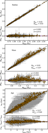 |
Fig. A.1 One-to-one relation and fractional differences from MAISTEP (ML) with respect to those from SPInS (Baye) in radius (top), mass (middle), and age (bottom). The dashed black lines in all panels represent the unity relation. The purple line in the fractional difference plots represents the median offset, μ. The horizontal grey bands highlights the associated scatter, ± σ. We also indicate the median fractional uncertainties in the one-to-one plots using σ̃. |
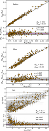 |
Fig. A.2 Same as Fig. A.1, but showing MAISTEP inferences using zero-point parallax corrections that depend on each star’s magnitude, colour, and position in the luminosity constraint, compared with the estimates from Fulton & Petigura (2018) for an overlapping sample of 236 stars. |
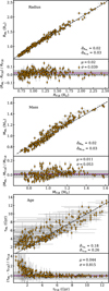 |
Fig. A.3 Same as Fig. A.2, but showing MAISTEP inferences using a fixed −0.053 zero-point parallax correction in the luminosity constraint, compared with the estimates from Fulton & Petigura (2018) for an overlapping sample of 236 stars. |
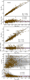 |
Fig. A.4 Same as Fig. A.2, but comparing to isochrone estimates of 587 stars in Berger et al. (2023a). |
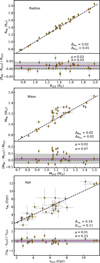 |
Fig. A.5 Same as Fig. A.2, but comparing to seismic estimates for 31 exoplanet host stars in Silva Aguirre et al. (2015). |
All Tables
Initial grid parameter ranges and input physics. ∆ refers to the step size in our Cartesian grid.
All Figures
|
Fig. 1 Kiel diagram showing 779 selected planet host stars overlaid on the main-sequence model grid (grey points). The marker shows median uncertainties of 0.05 dex in log g and 60 K in Teff. |
| In the text | |
|
Fig. 2 Top panel: histograms of planet radii from the literature (black) and our revised values (orange), using 0.33 R⊕ bin width. Dashed curves represent kernel density estimates (KDEs) computed with 0.33 R⊕ bandwidth. Lower panel: KDE distributions of radius uncertainties, with vertical dashed lines indicating the medians: 0.05 (this work) and 0.10 (literature values from the NASA Exoplanet Archive). |
| In the text | |
|
Fig. 3 Planet radius against orbital period. Small circles represent individual planet detections. Contours show the two-dimensional KDE of the planet population. The orange line is the best-fit trend, with a shaded band indicating the 68% confidence interval from bootstrap sampling. The error bar indicate the median uncertainty in planet radius. |
| In the text | |
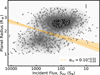 |
Fig. 4 Same as Fig. 3, except for planet size against incident flux. See text for details. |
| In the text | |
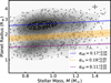 |
Fig. 5 Same as Fig. 3, but for planet size as a function of host star mass. See text for details. |
| In the text | |
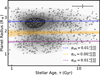 |
Fig. 6 Same as Fig. 3, but for planet size as a function of host star age. See text for details. |
| In the text | |
|
Fig. 7 Radius distributions of young (black) and old (orange) planets. Top: full population. Bottom: property-matched sample in stellar metal-licity, radius, and mass using optimal transport. Vertical dashed lines show the centroid of the inferred radius gap from GMM fits. Sample sizes, N, and ratios, NE/NN, are indicated in panel legends. |
| In the text | |
|
Fig. 8 Four-dimensional exoplanet radius valley across orbital period, stellar mass, and age space. Observed planets are overlaid, coloured by age, with sub-Neptunes (sNs) and super-Earths (sEs) distinguished by marker type. The fitted planes show the valley at representative ages of 2, 6, and 10 Gyr. |
| In the text | |
|
Fig. A.1 One-to-one relation and fractional differences from MAISTEP (ML) with respect to those from SPInS (Baye) in radius (top), mass (middle), and age (bottom). The dashed black lines in all panels represent the unity relation. The purple line in the fractional difference plots represents the median offset, μ. The horizontal grey bands highlights the associated scatter, ± σ. We also indicate the median fractional uncertainties in the one-to-one plots using σ̃. |
| In the text | |
|
Fig. A.2 Same as Fig. A.1, but showing MAISTEP inferences using zero-point parallax corrections that depend on each star’s magnitude, colour, and position in the luminosity constraint, compared with the estimates from Fulton & Petigura (2018) for an overlapping sample of 236 stars. |
| In the text | |
|
Fig. A.3 Same as Fig. A.2, but showing MAISTEP inferences using a fixed −0.053 zero-point parallax correction in the luminosity constraint, compared with the estimates from Fulton & Petigura (2018) for an overlapping sample of 236 stars. |
| In the text | |
|
Fig. A.4 Same as Fig. A.2, but comparing to isochrone estimates of 587 stars in Berger et al. (2023a). |
| In the text | |
|
Fig. A.5 Same as Fig. A.2, but comparing to seismic estimates for 31 exoplanet host stars in Silva Aguirre et al. (2015). |
| In the text | |
Current usage metrics show cumulative count of Article Views (full-text article views including HTML views, PDF and ePub downloads, according to the available data) and Abstracts Views on Vision4Press platform.
Data correspond to usage on the plateform after 2015. The current usage metrics is available 48-96 hours after online publication and is updated daily on week days.
Initial download of the metrics may take a while.