| Issue |
A&A
Volume 707, March 2026
|
|
|---|---|---|
| Article Number | A357 | |
| Number of page(s) | 12 | |
| Section | Numerical methods and codes | |
| DOI | https://doi.org/10.1051/0004-6361/202557556 | |
| Published online | 20 March 2026 | |
Integrated photogrammetry and photoclinometry for enhanced 3D surface reconstruction of asteroids
1
Research Centre for Deep Space Explorations | Department of Land Surveying & Geo-Informatics, The Hong Kong Polytechnic University, Hung Hom, Kowloon,
Hong Kong,
China
2
Beijing Institute of Spacecraft System Engineering, China Academy of Space Technology,
Beijing,
China
★ Corresponding authors: This email address is being protected from spambots. You need JavaScript enabled to view it.
; This email address is being protected from spambots. You need JavaScript enabled to view it.
Received:
4
October
2025
Accepted:
17
February
2026
Abstract
Stereo photogrammetry (SPG) and stereo photoclinometry (SPC) are the main techniques used in the 3D surface reconstruction of asteroids. The SPG approach retrieves accurate 3D geometry with limited spatial resolution, while SPC extracts fine-scale topography from image intensity but suffers from uncertainties in albedo and other factors. Integrating SPG and SPC therefore mitigates the limitations of each method when used alone. However, surface occlusions, illumination variations, and insufficient spatial coverage in asteroid observations pose challenges to integrated SPG–SPC. This paper presents an integrated photogrammetry and photoclinometry approach that leverages a pixel-weighted maplet (PWM) strategy specifically designed to address these challenges to obtain enhanced detailed 3D surface reconstruction of asteroids. The approach comprises four key steps: (1) reconstructing a sparse-resolution asteroid surface model using SPG, (2) generating PWMs by incorporating GPU-accelerated occlusion detection and an embedded optimal weighting strategy for image pixels to enable enhanced SPC refinement, (3) iteratively refining the surface of PWMs using SPC, and (4) assembling high-resolution PWMs into a complete global 3D model of the asteroid. We tested the developed method for 3D surface reconstruction of asteroids using actual images of the asteroid Bennu and images of a 3D-printed model of Bennu in a test field with controlled illumination and imaging settings. The results demonstrate that the proposed method achieves superior geometric accuracy and captures finer topographic details compared with state-of-the-art approaches. This development represents a notable advancement in high-fidelity asteroid modeling, offering critical support for future asteroid exploration missions and scientific research.
Key words: techniques: photometric / minor planets, asteroids: general / planets and satellites: surfaces
© The Authors 2026
 Open Access article, published by EDP Sciences, under the terms of the Creative Commons Attribution License (https://creativecommons.org/licenses/by/4.0), which permits unrestricted use, distribution, and reproduction in any medium, provided the original work is properly cited.
This article is published in open access under the Subscribe to Open model. This email address is being protected from spambots. You need JavaScript enabled to view it. to support open access publication.
1 Introduction
Surface reconstruction of asteroids in 3D is vital for asteroid exploration tasks such as identifying potential sampling sites (Walsh et al. 2022) and navigating mission spacecraft (Lauretta et al. 2017) as well as scientific research topics such as their geological evolution (Walsh et al. 2019). An asteroid’s physical properties can be inferred through analysis of its 3D model (Barnouin et al. 2019), enabling the simulation of an asteroid’s rotation and orientation that is essential for plotting spacecraft trajectories and avoiding obstacles (DellaGiustina et al. 2019). As even subtle topographic deviations can lead to possible mission failure, detailed surface reconstruction is essential when exploring asteroids (Veverka et al. 2001). To derive high-resolution topography, photogrammetry is the traditional approach to reconstructing the surface using stereo image pairs covering large overlapping areas (Li et al. 2022a). A photogrammetric model can achieve high geometric accuracy, but usually only sparse surface models can be generated. Photoclinometry is an alternative technique that extracts 3D surface information from surface-reflected light, represented by the image brightness (Wu et al. 2022). It has been applied to the shape modeling of numerous asteroids, including those surveyed during exploration missions (Palmer et al. 2022). Photoclinometry enables surface reconstruction for the extraction of pixel-wise details (e.g., of small rocks that are indiscernible by photogrammetry) from images; however, it suffers from uncertainties in albedo and issues due to other factors (Wu et al. 2021). Therefore, the integration of photoclinometry and photogrammetry as complementary methods could be a promising route to high-resolution and high-accuracy 3D reconstruction of asteroid surfaces.
Detailed 3D surface modeling of asteroids is nevertheless hindered by the scarcity of high-resolution images, as such data are primarily obtained through detailed surveys conducted by spacecraft or space probes (Durech et al. 2015). Furthermore, asteroid imagery is much more variable in quality than imagery of large planetary bodies. For instance, unlike large celestial bodies, most main-belt asteroids have diameters below 1 km (Tedesco et al. 2005); the viewing angle and illumination conditions thus vary significantly across asteroid observations. Changes in viewing direction and local surface curvature may lead to serious occlusions of some surface areas, obscuring detailed information in the images (DellaGiustina et al. 2018). In addition, the image scale changes considerably across different surveying phases and distances (Jaumann et al. 2016; Watanabe et al. 2017). An increase in spatial resolution at closer survey distances can result in a more pronounced curvature of the imaged asteroid surface, which in turn causes variations in the photometric geometry of each surface area within the image. Furthermore, the illumination at a given location can exhibit significant differences between images taken in different epochs (Jaumann et al. 2019), and obtaining global coverage of high-quality images from an asteroid is challenging due to limitations in imaging sequences.
This paper presents an integrated photogrammetrp–yhotoclinometry method for detailed 3D surface reconstruction of asteroids that leverages a pixel-weighted maplet (PWM) strategy specifically designed to address the above challenges. Section 2 provides a brief review of studies relevant to this topic. Section 3 details the approach for enhanced 3D surface reconstruction of asteroids. Section 4 describes the experimental validation of the approach and assesses the impact of optimal pixel weighting. Section 5 presents a discussion and our concluding remarks.
2 Related work
Stereo photogrammetry (SPG) is the technique of obtaining precise measurements from two or more photographs taken at different positions. It has been a pivotal tool in planetary science for creating 3D models from 2D spacecraft camera images (Wu 2017). Early applications of SPG in the production of topographic maps of small celestial bodies, such as that of the asteroid Eros during the NEAR Shoemaker exploration mission, enabled further engineering and scientific analyses (Thomas et al. 2002). The subsequent missions Hayabusa and Hayabusa2 visited the asteroids Itokawa and Ryugu and employed high-resolution imaging and SPG to reconstruct 3D shape models, revealing their rubble-pile structures and informing sample collection strategies (Fujiwara et al. 2006; Watanabe et al. 2019). Similarly, the impressive global mapping of comet 67P conducted during the Rosetta mission showcased the ability of SPG to precisely retrieve the surface topology of an extremely complicated irregularly shaped body (Preusker et al. 2017; Sierks et al. 2015). These endeavors highlight the reliability and importance of photogrammetric modeling in asteroid exploration, and they laid the foundation for analyzing the physical characteristics of small bodies and planning the subsequent mission at close range.
Photoclinometry allows for the retrieval of pixel-level 3D information from optical images with variable illumination taken under different lighting conditions. Monocular images can be used to recover detailed ground features by photoclinometry (Horn 1977; Wu et al. 2018). When multiple images are used in photoclinometric 3D reconstruction for enhanced performance, it is called stereo photoclinometry (SPC), and it is based on the photometric stereo technique, which analyzes the differences in intensity values between numerous observations of a location imaged under different illumination conditions, assuming that they share the same viewing direction and surface coverage (Woodham 1980; Liu et al. 2018). Gaskell et al. (2008) systematically applied SPC in the global reconstruction of shape models of asteroids such as Itokawa. Other missions have also used SPC as the primary technique to generate high-resolution shape models of asteroids (e.g., Bennu and Dimorphos) (Barnouin et al. 2019; Gaskell et al. 2023; Palmer et al. 2022; Terik Daly et al. 2022), supporting the detailed topographic and geomorphologic analysis of these small celestial bodies.
In recent years, deep learning has emerged as a highly prominent and widely researched method in 3D scene reconstruction, attracting attention to its application for planetary surface imaging. Early works explored the use of convolutional neural networks to directly predict height values using a single image and a coarse reference digital elevation model, enabling high-resolution reconstruction of the Martian surface (Chen et al. 2021; Tao et al. 2021). For modeling of the 3D topography of asteroids in complex scenarios, implicit neural representations can be used to jointly learn surface shape and brightness from images. Chen et al. (2024a) encoded the surface as a signed distance field and modeled the brightness as a radiance field, while Chen et al. (2024b) further used appearance embeddings to handle illumination variability between images. More recently, implicit neural techniques have been extended further to accomplish the shape modeling of the entire surface of an asteroid with refined terrain details based on only a limited number of images (Chen et al. 2025).
However, deep learning-based methods tend to smooth out the fine-scale details of an asteroid’s surface, including small rocks, concavities, and craters, which are essential in the later phases of mission planning and scientific research. Although this type of method requires only a limited number of images for 3D reconstruction, accurate initial input parameters of camera position and rotation are still needed, and training the deep learning model demands considerable effort and resources. Traditional methods such as photogrammetry can adjust the camera parameters and accurately estimate the 3D coordinates of surface points, while photoclinometry can reconstruct pixel-level terrain details under varied illumination conditions. The integration of these two techniques has been applied to large planetary bodies, such as the Moon and Mars (Li et al. 2022b; Liu & Wu 2020). For an asteroid, however, the shape can be very irregular, and the surface will likely be curved within the image frame. This leads to the loss of topographic information in the occluded and shadowed locations within a single image, necessitating multiple images under different viewing and lighting conditions. The method we present in this paper offers the following novel features compared to previous works:
(1) Occlusion detection incorporating GPU acceleration for enhanced 3D surface reconstruction of asteroids with diverse viewing geometries and a large surface curvature.
(2) Optimized consideration of the illumination incidence angle and azimuthal angular variations in images used for the SPC process.
(3) Correspondence between local image regions and the PWMs, which take into account illumination, shadow, occlusion, and image coverage for optimized SPC refinement.
3 Integrated photogrammetry–photoclinometry for 3D reconstruction of asteroids
3.1 Overview of the method
The overall workflow of the integrated photogrammetry–photoclinometry method for 3D surface reconstruction of asteroids is illustrated in Fig. 1. First, optical images of the observed asteroid and their corresponding interior orientation (IO) and exterior orientation (EO) parameters are set as the initial inputs for the overall approach. Using SPG, the EO parameters are optimized, and the disordered image sequences are matched to construct the initial asteroid shape model. Next, local surface patches are generated by transforming each part of the photogrammetric 3D surface model from the body-fixed coordinate system to the defined local coordinate system. Based on the topography of each local surface, the observation geometry of the corresponding images can be acquired from the optimized EO parameters. For images deeply affected by occlusion, a fast and accurate occlusion detection algorithm is developed to identify the obscured ground features. Additionally, with the assistance of the ephemeris data, the illumination geometry of each image corresponding to each local surface can be calculated. Then, image weighting and processing are performed to determine per-pixel priority and prepare the data for region-specific access while considering the factors addressed above. At this stage, the image intensity is aligned with the topography extracted from local surfaces to generate PWMs. Finally, pixel-level detail of the asteroid’s surface can be refined using the developed SPC method, incorporating the constraints embedded in the PWM.
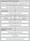 |
Fig. 1 Overview of the integrated photogrammetry–photoclinometry method for 3D reconstruction of asteroids. |
3.2 Photogrammetric and photoclinometric 3D reconstruction
Photogrammetry extracts an object’s geometric information from stereo pairs of images based on the collinear geometric relationship between the camera projection center, the original point in 3D space, and its corresponding image point on the image plane, linked by the IO and EO parameters. This collinear relationship enables stereo pairs to be used for reconstructing an asteroid’s 3D surface model through photogrammetric triangulation (Wu 2017). Photogrammetry retrieves highly accurate 3D geometric information from an asteroid surface via the structure-from-motion (SfM) and multi-view stereo (MVS) techniques. The SfM technique involves analyzing a sequence of images to estimate the camera parameters and reconstructing the sparse 3D geometry of an asteroid. Initially, the SfM pipeline extracts and matches the feature points on the surface of the asteroid to establish the correspondence across images. Subsequently, it estimates the IO and EO parameters of the camera and triangulates the 3D coordinates of matched feature points. Finally, the optimal camera parameters and sparse 3D point cloud of the asteroid are acquired through bundle adjustment optimization (Hu et al. 2016). Then, the MVS pipeline generates dense 3D reconstructions of the asteroid surface from the same set of images using the calibrated camera parameters and sparse reconstructions output by the prior SfM workflow. The MVS pipeline estimates the depth or 3D coordinates of the pixels in each image and conducts depth fusion by leveraging photometric consistency across multiple views to acquire a dense point cloud.
Photoclinometry reconstructs 3D shapes based on the photometric relationship between the illumination of a surface and the image intensity in a certain viewing direction (Kirk 1987; Liu & Wu 2023). The intensity of each pixel contains information on the interactions between the incoming radiation (e.g., sunlight) and the terrain (Gaskell et al. 2006). The photometric relationship can be modeled as
![Mathematical equation: $\[I=A G(p, q),\]$](/articles/aa/full_html/2026/03/aa57556-25/aa57556-25-eq1.png) (1)
(1)
where A is the albedo, an intrinsic property of a surface indicating its reflection of incident light, and G(p, q) is the reflectance from surface point z = S(x, y), where (x, y) are coordinates in the local coordinate system. The product of A and G yields the image intensity I perceived by the camera on board the space probe. The normal vector n is projected onto the x-direction and y-direction, yielding the vector components p and q, respectively. The surface gradient vector is the negative form of the surface normal vector, and these two normal vector components are defined as follows:
![Mathematical equation: $\[\begin{aligned}p & =-\frac{\partial z}{\partial x} \\q & =-\frac{\partial z}{\partial y}.\end{aligned}\]$](/articles/aa/full_html/2026/03/aa57556-25/aa57556-25-eq2.png) (2)
(2)
The value of G(p, q) is estimated by a reflectance model, which is typically chosen from among several widely used candidates (Golish et al. 2021), including the Lambertian, Lommel–Seeliger, Lunar–Lambertian (McEwen 1986), and Hapke models (Hapke 1981). In this study, we use the Lunar-Lambertian model to handle the retrieval of reflectance:
![Mathematical equation: $\[G(p, q)=(1-\phi(g)) \mu_0(p, q)+2 \phi(g) \frac{\mu_0(p, q)}{\mu_0(p, q)+\mu(p, q)}.\]$](/articles/aa/full_html/2026/03/aa57556-25/aa57556-25-eq3.png) (3)
(3)
Here, μ0(p, q) represents the cosine value of the incidence angle i and μ(p, q) represents the cosine value of the emission angle e. This empirical photometric model combines the Lambertian and Lommel–Seeliger models, introducing a function ϕ(g) to balance the two based on the phase angle g (the angle between the incident light direction and the viewing direction) (Hapke 2012). The objective of photometric refinement is therefore to minimize the residual (r) between the extracted and the predicted value of brightness:
![Mathematical equation: $\[r=(I-A G(p, q))^2.\]$](/articles/aa/full_html/2026/03/aa57556-25/aa57556-25-eq4.png) (4)
(4)
By introducing Equations (1)–(3) into equation (4), the albedo is estimated while the two partial derivatives (p, q) are updated. Finally, the position of a surface point is adjusted according to that of its neighboring points using gradients from the updated (p, q) (McEwen 1991).
However, the above standard photoclinometric process relies on images of relatively flat terrain and is therefore ill-suited for reconstructing an asteroid’s surface. Hence, the PWM was developed to overcome this limitation.
 |
Fig. 2 Conceptual illustration of PWM construction. |
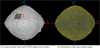 |
Fig. 3 (a) Example of a sparse global asteroid model (light gray) and a PWM (dark gray). The associated coordinate systems are represented by the solid lines (global body-fixed system) and dashed lines (local PWM-fixed system). (b) Partitioning of the global model for generating thousands of PWMs. |
3.3 Generation of pixel-weighted maplets
During iterative photoclinometric refinement, each PWM serves as the basic reconstruction element. Image intensity, image weights, and terrain data are fused within these PWMs to resolve surface properties at per-pixel resolution (Fig. 2). The PWM is specifically designed to connect photogrammetry and photoclinometry in this study. Each PWM provides not only the photogrammetrically derived topography of local surface patches but also the analyzed image information for optimal surface reconstruction of an asteroid.
3.3.1 Partitioning of the sparse global model for generation of PWMs
The photogrammetric model of the entire asteroid cannot be directly used for photoclinometry; thus, the global model is divided into numerous regional surface models (Fig. 3). Each model within a square area is defined as a PWM-aligned surface, whose size is determined by the image resolution and the shape of the asteroid. The original photogrammetric model is associated with the asteroid’s body-fixed coordinate system, making it challenging to modify the height of local surface points. Thus, local coordinate systems (Fig. 3) are established for each PWM-aligned local surface to guide all subsequent processes.
The origin of the local coordinate system is located at the regional surface center, P0. The z-axis of the local coordinate system is defined by the regional surface normal vector vz. The x-axis (vx) is chosen to be parallel to the equator, and the y-axis (vy) is then determined by the right-hand rule. The transformation from global coordinates (P) to local coordinates (Pl) is defined as follows:
![Mathematical equation: $\[P_l=\left[\begin{array}{l}v_x \\v_y \\v_z\end{array}\right]\left(P-P_0\right).\]$](/articles/aa/full_html/2026/03/aa57556-25/aa57556-25-eq5.png) (5)
(5)
The regional surfaces are then generated by facilitating the global-to-local transformation of original points within the defined regions.
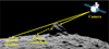 |
Fig. 4 Illustration of the occlusion problem. Point A is occluded by a boulder, while point B is directly observed by the camera. Yellow lines indicate the line-of-sight viewing rays. |
3.3.2 GPU-accelerated ray tracing for occlusion detection
During the surveying phase of an asteroid by optical photography, the captured surface images are very likely to have occluded areas. As the image processing procedure registers image pixels to the PWM-aligned local surface, the surface points occluded by nearby ground features should be removed from the image to minimize the negative impact of invalid intensity values on the shape modeling. A GPU-accelerated ray tracing algorithm has been developed to efficiently identify occluded surface points in images, addressing the prohibitive computational cost for per-point visibility validation when dealing with high-resolution datasets. The observation geometry is first calculated for each image based on the local surface, followed by analysis of the occlusion problem (Alsadik et al. 2014). If the line-of-sight ray starts with an image (or camera position) intersected by any part of the surface before the target point, that target point is considered to be occluded (Fig. 4). Otherwise, the target point is visible on the image and can contribute to the subsequent reconstruction process. This visibility-checking module is implemented into the image processing pipeline; Fig. 5 shows the results for two regions with invalid pixels removed.
3.3.3 Optimal weighting for image pixels of PWMs
The performance of the photoclinometry method employed in this study is influenced by both the quality and quantity of the available images. An image weighting procedure was conducted to assign weights to each image pixel, corresponding to regional 3D surface models within their respective frames, thereby balancing the contributions of individual images. The previously calculated viewing geometry was first used to identify all images covering a PWM region and aligned their pixels with the region. Fig. 6 depicts a simplified representation of the illumination and observation geometry. The spatial configuration of objects, including the light source, illuminated surface, and observer, can be represented by the incidence angle i and the emission angle (or viewing angle) e, defined relative to the normal vector n of the surface.
To conduct a quality assessment, the viewing angle of an image was analyzed, and the proportion of the obscured area was calculated by the ray tracing algorithm outlined in the preceding section. The incidence angle between the incoming light direction and the surface normal vector was also quantified using the illumination geometry originating from the ephemeris data. Our previous work (Liu & Wu 2021) indicated that the optimal solar incidence angle for photoclinometric 3D reconstruction is in the range of 30°–60°. Having too large of an incidence angle results in severe shadows, which hide topographic details, whereas having an incidence angle that is too small reduces the contrast on surface slopes and therefore compromises the ability to resolve fine surface details. An optimal angle of incident light enables both accurate photometric estimation and an acceptable proportion of shadowed area. To this end, each image is assigned a light incidence weight (or incidence-dependent weight) to indicate the importance of the image based on the incidence angle. During this process, shadows can be detected and excluded, as shadowed areas typically receive negligible scattered and reflected light considering the low surface albedo and atmosphere-free properties of asteroids. In some scenarios involving special challenges, including drastic elevation changes or the presence of high albedo features adjacent to areas not exposed to direct solar radiation, shadows will be allocated a small weight rather than being ignored entirely.
The SPC method used in this study requires multi-view images, and the diverse viewing angles and comprehensive terrain coverage in them are critical for robust reconstruction. To conduct a quantity assessment, each image was analyzed for both its sufficiency in supporting surface refinement and the spatial coverage of its co-registered maplet regions. To ensure sufficient surface observation, in this study, each PWM was suggested to be supported by at least five overlapping images acquired from distinct viewing geometries, namely, east, west, north, south, and nadir perspectives. The selected nadir image is the one with the lowest phase angle and smallest proportion of occluded areas, assisting the optimization of initial parameter estimation during photoclinometric processing. The other four images were selected from the imagery database based on the calculated viewing direction. These images provide complementary perspectives and illumination of azimuthal variations (Liu et al. 2018), as required for SPC reconstruction. The azimuthal variation of the solar incidence was also calculated to determine whether it is below 90 degrees within a maplet image set. If an insufficient number of images met either the perspective or illumination requirements, the corresponding maplet was assigned a lower regional weight to reduce its influence on the refined terrain.
The intensity recorded by each image pixel was matched to local surface points along with the corresponding illumination and observation geometry. Furthermore, other key information, including the constraining weights assigned to each image–region association, was aligned with the pixel nodes. A PWM, as a bridging unit, was then derived from the existing local surface model to establish connections among all terrain-related information for each point (or pixel). Moreover, if qualitative and quantitative assessments indicated inadequate imagery for a maplet region, a reduced weighting factor, based on the effective spatial coverage and lighting conditions of the region’s imagery, could be embedded in the PWM. This region-dependent weight is introduced into the photoclinometric reconstruction to constrain adjustments to the initial surface model.
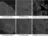 |
Fig. 5 Results of visibility checking (each row corresponds to one region). Panels (a) and (d) are the original images (20190419T202633S865_map; 20190516T213136S334_map), and the gray box indicates the location of the region. Panels (b) and (e) are the PWM-aligned images containing the occluded pixels. Panels (c) and (f) are the PWM-aligned images with occluded pixels removed (black pixels). |
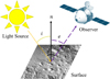 |
Fig. 6 Simplified illustration of the illumination and observation geometry. |
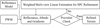 |
Fig. 7 Overall workflow of the photoclinometric surface refinement approach. |
3.4 Photoclinometric 3D surface refinement of PWMs
The SPC refinement approach (Fig. 7) in this work iterates the maplet’s surface properties through a weighted multi-view linear estimation to achieve pixel-level surface refinement of the PWM. By integrating the reflectance model with the PWM derived from the photogrammetric 3D model, this approach estimates the albedo and gradients. A precision check of the estimates is then conducted. After determining that the process has converged to an optimal estimation of the refined albedo and gradients, the position of each surface point is adjusted to represent the asteroid’s topographic details.
The photoclinometric refinement process is conducted on the PWMs, which contain the initial terrain information acquired through photogrammetric stereo products that provide an overall accuracy constraint to assist high-resolution modeling of the asteroid. With this photogrammetric model, the original inputs of the normal vector derivatives (p0, q0) can be calculated.
The SPC reconstruction pipeline uses both photogrammetric stereo and photometric stereo images to provide the various viewing geometries and illumination geometries that are required. These images are aligned to the PWM, while the brightness of each image pixel is connected with the surface reflectance through Equation (1). The image pixels connected to the same surface point are then grouped to obtain the optimized albedo and terrain by minimizing the following equation:
![Mathematical equation: $\[r=\sum_k(w_k(I_k-A G_k(p, q)))^2,\]$](/articles/aa/full_html/2026/03/aa57556-25/aa57556-25-eq6.png) (6)
(6)
where k is the number of images used in the linear estimation approach and wk is the weight assigned to each image based on the image analysis results. This equation serves as the intensity constraint for terrain adjustment. Additionally, an integrability constraint is added to prevent ill-posed recovery of normal vectors, while a surface normal constraint ensures that the refined terrain does not deviate excessively from the photogrammetrically constrained shape:
![Mathematical equation: $\[\begin{aligned}r= & \sum_k(w_k(I_k-A G_k(p, q)))^2+w_i(p_y-q_x)^2 \\& {+}\frac{1}{w_{P W M}}((p-p_0)^2+(q-q_0)^2),\end{aligned}\]$](/articles/aa/full_html/2026/03/aa57556-25/aa57556-25-eq7.png) (7)
(7)
where ![Mathematical equation: $\[p_{y}=-\frac{\partial p}{\partial y}\]$](/articles/aa/full_html/2026/03/aa57556-25/aa57556-25-eq8.png) and
and ![Mathematical equation: $\[q_{x}=-\frac{\partial q}{\partial x}\]$](/articles/aa/full_html/2026/03/aa57556-25/aa57556-25-eq9.png) . The integrability term is also assigned an empirical weight wi to control how strictly the slope field is enforced to be integrable. The differences in image quality and image sufficiency between PWMs are significant; hence, a region-dependent weight wPWM is determined for each PWM to control the relative strength of the surface normal constraint with respect to the image-derived normals.
. The integrability term is also assigned an empirical weight wi to control how strictly the slope field is enforced to be integrable. The differences in image quality and image sufficiency between PWMs are significant; hence, a region-dependent weight wPWM is determined for each PWM to control the relative strength of the surface normal constraint with respect to the image-derived normals.
3.5 Fusion of PWMs for generating the global 3D surface model
To mitigate occlusions caused by pronounced surface curvature, the detailed surface is reconstructed on the small surface patch defined in each PWM. The size of a PWM, as well as the degree of overlap between adjacent PWMs, is dictated by image coverage and the asteroid’s shape. A detailed 3D surface model of the asteroid is then generated through PWM fusion using photoclinometrically refined maplets. Prior to fusion, all refined PWMs are projected into a common space. The partially overlapping PWMs are not realigned at this stage, as a rigid transformation is applied between the asteroid body-fixed reference frame and each local PWM-fixed coordinate system to maintain photogrammetrically constrained geometric accuracy.
The details in overlapping regions are slightly inconsistent due to the varied image adequacy of each PWM. Direct surface reconstruction of these regions could produce topographic artifacts, and therefore a voxel fusion technique (Li et al. 2019) is employed to resolve discrepancies while preserving the improved details. The overlapping 3D surface is discretized into sufficiently small voxels, and a weighted average method using the region-dependent weights then merges adjacent vertices within each voxel during fusion. Smoothness and consistency across the entire surface are ultimately maintained after fusing all PWMs and remeshing the detailed 3D surface model.
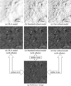 |
Fig. 8 Detailed comparison of 3D models within the same region. Panel (a) shows the surface of the OLAv21PTM LiDAR-based 3D model. Panels (b) and (c) show our reconstructed surface refined through the standard method and proposed method, respectively. Panels (d)–(f) indicate the albedo rendering results for (a)–(c). Panel (g) shows a representative image (20190321T203010S305_pol) taken from a near-nadir direction. |
4 Experimental analysis
We acquired the dataset for reconstructing an asteroid shape model from the NASA Planetary Data System (PDS) archive of the OSIRIS-REx exploration mission. The image data were taken by the OSIRIS-REx Camera Suite, a set of three cameras (PolyCam, MapCam, and SamCam) designed to capture the asteroid Bennu at varying distances and resolutions (Rizk et al. 2018). The ephemeris data used here were retrieved from the OSIRIS-REx SPICE kernels (Semenov et al. 2023), assisting in the calculation of imaging geometry and lighting geometry. The space probe also hosts a light detection and ranging (LiDAR) apparatus called the OSIRIS-REx Laser Altimeter (OLA) (Seabrook et al. 2019). The two best shaped models of the asteroid Bennu from the OLA laser scanning (Seabrook et al. 2022) and the SPC reconstruction (Al Asad et al. 2021; Palmer et al. 2024) are also available in the PDS archive. We compared the shape model reconstructed through the approach proposed in this study with these two models to evaluate its performance and accuracy in 3D surface reconstruction.
4.1 Comparative evaluation between standard SPC method and the proposed method
The reconstruction test, performed on a typical region of the asteroid Bennu, focuses on the optimized photoclinometric reconstruction method using PWM-aligned weighted image pairs while considering the impact of observation and illumination geometries on the reconstructed surface. The SPC process involves estimating surface normal vectors and albedo via intensity information from the weighted image pairs (with resolution ranging from 0.05 to 0.07 m) to generate a detailed 3D surface model. To conduct a performance assessment of the proposed method, a shape model was reconstructed using a standard photoclinometric approach (Liu et al. 2018) for comparison, but we excluded the image-dependent weights and a region-dependent weight.
Figure 8 compares the terrain details of a region (with a size of 14 m) from different 3D models and a selected reference image, with the surface of these models illuminated under the same lighting condition as in the reference image. Both of our generated 3D models exhibit remarkably detailed surface features compared with the LiDAR-based 3D model. The 3D models were further rendered with the same estimated geometric albedo, and the resulting images were assessed using the structural similarity index (SSIM) in order to analyze their rendering quality.
The SSIM is a quantitative metric for the similarity between a reference image and a test image, producing a value between zero and one. An SSIM score closer to zero indicates less similarity, while a score nearer one indicates greater similarity. In comparison with the reference image in Fig. 8, the rendered images demonstrate some notable differences in the surface features, and the quality of the surface reconstruction by our proposed method surpasses that of the standard method. The proposed method also yields more accurate representations of the illuminated surface than the reference image, as shown by an SSIM value of 0.80. Meanwhile, the OLA model and standard-method model achieve SSIM scores of 0.55 and 0.60, respectively, which is significantly lower than our proposed method.
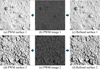 |
Fig. 9 Simplified example of the photoclinometric refinement. Panels (a) and (d) show two different PWM-aligned surfaces at relatively low resolution. Panels (b) and (e) are representative of the aligned images for these two PWMs. Panels (c) and (f) are the refined surfaces with pixel-level detail. |
4.2 Evaluation using real images of asteroid Bennu
Approximately 8000 high-resolution images (with resolutions ranging from 0.05 to 0.07 m per pixel) from the PolyCam generated during the detailed surveying phase (Barnouin et al. 2020) were used in this study, providing detailed and complete observation of the Bennu asteroid’s global topography. Fig. 9 shows the photoclinometry-refined local surface based on the photogrammetry-constrained model using a PWM of 30 m in size. The terrain-dependent reflectance has been adjusted to minimize the difference between the estimated and the observed intensity of each connected image, resulting in a high-resolution and detailed surface within each PWM. The first PWM (Figs. 9a and 9b) corresponds to a relatively smooth region on the asteroid Bennu mainly covered by gravel or fine-grained regolith. The second PWM (Figs. 9d and 9e) represents a topographically heterogeneous region dominated by boulders with irregular shapes and diverse size distributions. As demonstrated by the results, the approach performs effectively on surfaces characterized by subtle details (Fig. 9c) as well as those crowded with boulders (Fig. 9f).
The customized size of the PWM generated in this experiment was set to 30 m, leading the complete global surface of the Bennu asteroid to be separated into around 1300 blocks of PWMs. The surface details of all PWMs were subsequently enhanced through the photoclinometric reconstruction pipeline. These refined topographic datasets were then merged into one cohesive global representation of the asteroid’s entire surface (Fig. 10). To analyze the performance of the proposed approach, a LiDAR-based shape model (OLAv21PTM) was employed as the reference for analytical and quantitative verification of our shape model. Additionally, an SPC-based shape model (SPCv42) was selected for comparison with our model, as both models implement the photoclinometry technique to reconstruct high-level surface details.
Figure 11 illustrates the differences in detail between each model at the global and regional scales. The SPCv42 model accurately represents the overall shape of the asteroid, but it compromises details at scales ranging from several centimeters to a few meters, causing such details to be scarcely visible on the surface. Relative to the reference model, the reconstruction by our model retains a high quality in terms of both global morphology and subtle regional details while achieving a spatial resolution of up to 0.05 m, surpassing that of the reference model. To facilitate comparison with the SPCv42 model, the facet count of our detailed model was downsampled from 1.67 billion to 3 million to match that of the SPCv42 model. The result demonstrates that the fine-scale features in both our high-resolution model and the down-sampled model closely resemble those of the reference model, whereas the same region appears markedly smoother in the SPCv42 model.
We further evaluated the topographic consistency of the shape models in terms of their morphological fidelity to the reference model. Fig. 12 depicts a notably large boulder whose size and complex morphology introduce difficulty in observing it and its surroundings due to the occlusion problem and shadows. The downsampled model was used here to emphasize the importance of the photogrammetric constraint provided by each PWM. The SPG technique embedded in our approach lays the foundation for accurately reconstructing this kind of ground feature and constraining the subsequent photoclinometric refinement process. The boulder’s overall morphology in our model matches the reference model with high fidelity, in contrast to the SPCv42 model, where there exists a large deviation from the supposed shape.
The two SPC-based 3D surface models were compared for their accuracy by measuring pointwise distances (or deviations) between the evaluated surface and the reference surface. Fig. 13 maps the topographic errors of both models across the entire surface, utilizing a color scheme where red and yellow gradients denote overestimated heights and blue and green gradients indicate underestimated heights relative to the reference surface. Our reconstructed asteroid body was mapped with uniform coloration, demonstrating that high geometric accuracy is maintained by our approach. In contrast, heterogeneous color distributions across the surface of the SPCv42 model reveal systematic global terrain deviations, especially in rough regions. The differences between the SPC-based 3D surface models are statistically quantified in Table 1, summarizing the meter-level maximum errors, which for both shape models appear on the edges of large ground features such as boulders. Their overall errors are reasonably small, at the submeter scale, with our model achieving a root mean square deviation (RMSD) of 0.31 m, approximately half that of the SPCv42 model (0.64 m).
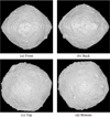 |
Fig. 10 Surface model of the asteroid Bennu in 3D reconstructed through our proposed approach. Panels (a) and (b) depict front and back views with the viewing point located on the equatorial plane. Panels (c) and (d) show the northern hemisphere and southern hemisphere, respectively. |
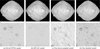 |
Fig. 11 Comparison of surface details of asteroid Bennu from different 3D surface models. Panel (a): NASA OLAv21PTM reference model formed by 18 million facets. Panel (b): NASA SPCv42 model formed by 3 million facets. Panel (c): our down-sampled model formed by 3 million facets. Panel (d): our detailed model formed by 1.67 billion facets. |
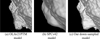 |
Fig. 12 Illustration of the topographic deviation of different 3D surface models of the asteroid Bennu. A large boulder is imaged by three models: (a) the OLAv21PTM model, the (b) SPCv42 model, and (c) our down-sampled model. |
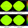 |
Fig. 13 Accuracy comparison of photoclinometry-based 3D surface models relative to the reference model. Panels (a) and (b) represent the deviation of the SPCv42 model from the reference. Panels (c) and (d) represent the deviation of our model from the reference. |
Statistics of the deviations of the photoclinometry-based 3D surface models.
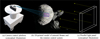 |
Fig. 14 Indoor test field for simulating an in situ observation. |
4.3 Evaluation using images taken in a controlled testing site
Pre-arrival validation of the algorithm is essential, as demonstrated by prior work validating similar algorithms for asteroid Bennu during the OSIRIS-REx mission (Craft et al. 2020). In this experiment, approximately 7000 images were acquired from a controlled indoor test site simulating in situ observation of asteroids. As illustrated in Fig. 14, the test field was constructed in a dark indoor environment to avoid interference from other light sources, such as solar radiation. A light panel was built to provide parallel light to simulate solar illumination on a 3D-printed model (based on the public model OLAv20PTM of the asteroid Bennu (Daly et al. 2020)) of an asteroid placed in the center of the test field. The test model is 1.5 m in diameter, and a rotation simulation system was designed to move and rotate this test model according to experimental requirements. Meanwhile, a camera platform followed an in-orbit observation plan to capture images of the model. The test images (with a resolution of approximately 0.7 mm per pixel) and corresponding pose data were used for detailed 3D reconstruction to validate the effectiveness of the developed algorithm and the feasibility of the imaging strategy. To verify the accuracy of the reconstructed 3D model, a LiDAR scanner was employed during the simulation to comprehensively scan the model’s surface (achieving a 3D point accuracy of around 1.9 mm). The resulting point cloud data was regarded as the reference benchmark for quantitative comparison against the reconstructed 3D model.
Validation of the overall proposed approach follows the method outlined in the previous section. First, SPG was applied using images from multiple surveying stations to calculate the point coordinates of the test model 3D surface, which yielded an initial 3D model with a relatively coarse resolution. However, the rotation simulation device and the model were connected at an incomplete surface in the arctic region; hence, this region was cropped and removed from the reconstructed 3D model. The PWMs were then generated from the cropped SPG model to enable detailed surface refinement via photoclinometry algorithms. Finally, the detailed global topography could be derived by integrating these PWM outputs.
Figure 15 depicts the performance of the developed method, showcasing the fine-scale terrain detail on the reconstructed model’s surface compared with the reference image. The photoclinometric refinement process resolved pixel-level topographic variations (of about 1 mm), wherein the initial SPG 3D surface model lacked sufficient resolution. The difference between the initial and final models as shown in the terrain profiles reveals this improvement. The effectiveness of the proposed approach is also evident in Fig. 16, which provides a global visualization of the reconstructed 3D models compared with the reference model.
The final 3D surface model was further analyzed by calculating its surface deviation relative to the reference model (Fig. 17). The global deviation distribution shows that most differences fall within ±2 mm, with these areas predominantly displayed in green according to the color scale. Further statistical analysis (Table 2) corroborates this distribution of deviation values, as our final model achieves an RMSD of 0.81 mm. By contrast, the initial model shows an RMSD of 0.99 mm, indicating that our photoclinometric refinement process improves the overall accuracy of the initial sparse 3D surface model. In summary, our photogrammetry–photoclinometry integrated approach successfully reconstructs a detailed 3D surface of the asteroid test model with images captured under simulated observation conditions.
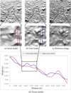 |
Fig. 15 Performance of the final model in fine-scale detail reconstruction. |
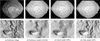 |
Fig. 16 Comparison of different 3D surface models of the asteroid test model. |
Statistics of the accuracy of the 3D surface reconstruction of the test model.
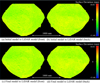 |
Fig. 17 Accuracy of the reconstructed 3D models compared with the LiDAR reference model. |
5 Discussion and conclusions
Through this paper, we have presented a photogrammetry–photoclinometry integrated approach utilizing PWMs for optimal pixel-level 3D topography mapping of asteroids. As an initial step, we constructed a lower-resolution photogrammetric 3D surface model to establish and maintain global geometric accuracy. This model subsequently served as the geometric foundation for generating PWMs, ensuring precise co-registration of terrain geometry and weighted image information. Then, the photoclinometry method was implemented for each PWM to ultimately realize the fine-scale refinement of an asteroid’s entire surface. The PWMs, as the key element of the approach, were developed to not only enable the asteroid’s 3D surface reconstruction but also enhance the performance of the algorithm. For each PWM, given the complicated geometries of the observation and illumination, specifically designed image weighting and experimental assessment processes were essential for determining the most suitable strategy for photoclinometric refinement. The assessment results showed that the developed strategy is more effective than comparison methods, laying the foundation for the detailed reconstruction of asteroids.
The developed method demonstrates robust 3D surface modeling of asteroids and leverages thousands of diverse high-resolution images. Experimental analyses of the overall approach using images of the asteroid Bennu with various viewing and lighting geometries confirmed that the proposed approach is capable of reconstructing a high-fidelity 3D surface model of an asteroid. The method exceeds the performance of the SPC-based 3D model (SPCv42) generated for the corresponding mission while delivering higher-resolution terrain detail than the LiDAR-derived 3D model (OLAv21PTM). Subsequently, we conducted an experiment at an indoor test site to validate the reliability of the method, using test images acquired from simulated in-orbit observation scenarios. The fine-scale reconstruction of the test asteroid model was successful, and its RMSD value is 0.81 mm with respect to the LiDAR model.
The significance of our integrated approach lies in the high fidelity across all scales, from regional to global. In the experiment using images of the asteroid Bennu, both the PWM regional surface and the asteroid’s global surface have RMSD values (i.e., deviations) of about 0.3 m relative to the LiDAR model. The highest spatial resolution we achieved for asteroid surfaces was 0.05 m, while certain regions were modeled at a coarse spatial resolution of 0.07 m, depending on the terrain details captured in the original images. The proposed approach thus enables pixel-wise 3D surface reconstruction of asteroids, which will support future planning of asteroid exploration missions and detailed analysis of scientific research. Future developments may extend to automated highfidelity 3D reconstruction of highly irregular small celestial bodies.
Data availability
The image data of the asteroid Bennu and the corresponding OSIRIS-REx SPICE kernels we used in this study are available from NASA PDS archives (https://sbnarchive.psi.edu/pds4/orex/orex.ocams/ and https://naif.jpl.nasa.gov/pub/naif/pds/pds4/orex/). The public 3D shape models can be found in the Small Body Mapping Tool (http://sbmt.jhuapl.edu/), which is also released to the NASA PDS archive. The dataset for our method is publicly available at https://zenodo.org/records/18732514.
Acknowledgements
This work was supported by grants from the Research Grants Council of Hong Kong (Project No.: 15219821; Project No.: 15215822). We would like to extend our appreciation to those who made the experimental data publicly available.
References
- Al Asad, M. M., Philpott, L. C., Johnson, C. L., et al. 2021, Planet. Sci. J., 2, 82 [NASA ADS] [CrossRef] [Google Scholar]
- Alsadik, B., Gerke, M., & Vosselman, G. 2014, ISPRS Ann. Photogramm. Remote Sens., II-5, 9 [Google Scholar]
- Barnouin, O. S., Daly, M. G., Palmer, E. E., et al. 2019, Nat. Geosci., 12, 247 [Google Scholar]
- Barnouin, O. S., Daly, M. G., Palmer, E. E., et al. 2020, Planet. Space Sci., 180, 104764 [NASA ADS] [CrossRef] [Google Scholar]
- Chen, Z., Wu, B., & Liu, W. C. 2021, Remote Sens., 13, 839 [NASA ADS] [CrossRef] [Google Scholar]
- Chen, H., Hu, X., Willner, K., et al. 2024a, ISPRS J. Photogramm. Remote Sens., 212, 122 [Google Scholar]
- Chen, S., Wu, B., Li, H., Li, Z., & Liu, Y. 2024b, A&A, 687, A278 [NASA ADS] [CrossRef] [EDP Sciences] [Google Scholar]
- Chen, H., Willner, K., Ziese, R., et al. 2025, A&A, 696, A212 [NASA ADS] [CrossRef] [EDP Sciences] [Google Scholar]
- Craft, K. L., Barnouin, O. S., Gaskell, R., et al. 2020, Planet. Space Sci., 193, 105077 [Google Scholar]
- Daly, R. T., Bierhaus, E. B., Barnouin, O. S., et al. 2020, Geophys. Res. Lett., 47, e89672 [NASA ADS] [CrossRef] [Google Scholar]
- DellaGiustina, D. N., Bennett, C. A., Becker, K., et al. 2018, Earth Space Sci., 5, 929 [Google Scholar]
- DellaGiustina, D. N., Emery, J. P., Golish, D. R., et al. 2019, Nat. Astron., 3, 341 [Google Scholar]
- Durech, J., Carry, B., Delbo, M., Kaasalainen, M., & Viikinkoski, M. 2015, Asteroid Models from Multiple Data Sources (University of Arizona Press), 183 [Google Scholar]
- Fujiwara, A., Kawaguchi, J., Yeomans, D. K., et al. 2006, Science, 312, 1330 [NASA ADS] [CrossRef] [Google Scholar]
- Gaskell, R., Barnouin-Jha, O., Scheeres, D., et al. 2006, in AIAA/AAS Astrodynamics Specialist Conference and Exhibit (American Institute of Aeronautics and Astronautics), 6660 [Google Scholar]
- Gaskell, R. W., Barnouin-Jha, O. S., Scheeres, D. J., et al. 2008, Meteorit. Planet. Sci., 43, 1049 [NASA ADS] [CrossRef] [Google Scholar]
- Gaskell, R. W., Barnouin, O. S., Daly, M. G., et al. 2023, Planet. Sci. J., 4, 63 [NASA ADS] [CrossRef] [Google Scholar]
- Golish, D. R., DellaGiustina, D. N., Li, J. Y., et al. 2021, Icarus, 357, 113724 [NASA ADS] [CrossRef] [Google Scholar]
- Hapke, B. 1981, J. Geophys. Res. Solid Earth, 86, 3039 [NASA ADS] [CrossRef] [Google Scholar]
- Hapke, B. 2012, Theory of Reflectance and Emittance Spectroscopy, 2nd edn. (Cambridge: Cambridge University Press) [Google Scholar]
- Horn, B. K. P. 1977, Artif. Intell., 8, 201 [Google Scholar]
- Hu, H., Ding, Y., Zhu, Q., et al. 2016, ISPRS J. Photogramm. Remote Sens., 118, 53 [Google Scholar]
- Jaumann, R., Schmitz, N., Koncz, A., et al. 2016, Space Sci. Rev., 208, 375 [Google Scholar]
- Jaumann, R., Schmitz, N., Ho, T. M., et al. 2019, Science, 365, 817 [NASA ADS] [CrossRef] [Google Scholar]
- Kirk, R. L. 1987, Thesis, California Institute of Technology [Google Scholar]
- Lauretta, D. S., Balram-Knutson, S. S., Beshore, E., et al. 2017, Space Sci. Rev., 212, 925 [Google Scholar]
- Li, Y., Wu, B., & Ge, X. 2019, ISPRS J. Photogramm. Remote Sens., 153, 151 [Google Scholar]
- Li, Z., Wu, B., Liu, W. C., et al. 2022a, IEEE Trans. Geosci. Remote Sens., 60, 4601096 [Google Scholar]
- Li, Z., Wu, B., Liu, W. C., & Chen, Z. 2022b, IEEE Trans. Geosci. Remote Sens., 60, 4601113 [Google Scholar]
- Liu, W. C., & Wu, B. 2020, ISPRS J. Photogramm. Remote Sens., 159, 153 [NASA ADS] [CrossRef] [Google Scholar]
- Liu, W. C., & Wu, B. 2021, ISPRS J. Photogramm. Remote Sens., 182, 208 [NASA ADS] [CrossRef] [Google Scholar]
- Liu, W. C., & Wu, B. 2023, ISPRS J. Photogramm. Remote Sens., 204, 237 [Google Scholar]
- Liu, W. C., Wu, B., & Wöhler, C. 2018, ISPRS J. Photogramm. Remote Sens., 136, 58 [NASA ADS] [CrossRef] [Google Scholar]
- McEwen, A. S. 1986, J. Geophys. Res. Solid Earth, 91, 8077 [Google Scholar]
- McEwen, A. S. 1991, Icarus, 92, 298 [Google Scholar]
- Palmer, E. E., Gaskell, R., Daly, M. G., et al. 2022, Planet. Sci. J., 3, 102 [NASA ADS] [CrossRef] [Google Scholar]
- Palmer, E. E., Weirich, J. R., Gaskell, R. W., et al. 2024, Planet. Sci. J., 5, 46 [Google Scholar]
- Preusker, F., Scholten, F., Matz, K. D., et al. 2017, A&A, 607, L1 [NASA ADS] [CrossRef] [EDP Sciences] [Google Scholar]
- Rizk, B., Drouet d’Aubigny, C., Golish, D., et al. 2018, Space Sci. Rev., 214, 26 [Google Scholar]
- Seabrook, J. A., Daly, M. G., Barnouin, O. S., et al. 2019, Planet. Space Sci., 177, 104688 [Google Scholar]
- Seabrook, J. A., Daly, M. G., Barnouin, O. S., et al. 2022, Planet. Sci. J., 3, 265 [Google Scholar]
- Semenov, B. V., Costa Sitja, M., & Bailey, A. M. 2023, OSIRIS-REx SPICE Kernel Archive Bundle [Google Scholar]
- Sierks, H., Barbieri, C., Lamy, P. L., et al. 2015, Science, 347, aaa1044 [Google Scholar]
- Tao, Y., Muller, J.-P., Xiong, S., & Conway, S. J. 2021, Remote Sens., 13, 4220 [NASA ADS] [CrossRef] [Google Scholar]
- Tedesco, E. F., Cellino, A., & Zappalá, V. 2005, AJ, 129, 2869 [Google Scholar]
- Terik Daly, R., Ernst, C. M., Barnouin, O. S., et al. 2022, Planet. Sci. J., 3, 207 [Google Scholar]
- Thomas, P. C., Joseph, J., Carcich, B., et al. 2002, Icarus, 155, 18 [NASA ADS] [CrossRef] [Google Scholar]
- Veverka, J., Farquhar, B., Robinson, M., et al. 2001, Nature, 413, 390 [NASA ADS] [CrossRef] [Google Scholar]
- Walsh, K. J., Jawin, E. R., Ballouz, R. L., et al. 2019, Nat. Geosci., 12, 242 [NASA ADS] [CrossRef] [Google Scholar]
- Walsh, K. J., Bierhaus, E. B., Lauretta, D. S., et al. 2022, Space Sci. Rev., 218, 20 [Google Scholar]
- Watanabe, S.-i., Tsuda, Y., Yoshikawa, M., et al. 2017, Space Sci. Rev., 208, 3 [Google Scholar]
- Watanabe, S., Hirabayashi, M., Hirata, N., et al. 2019, Science, 364, 268 [NASA ADS] [Google Scholar]
- Woodham, R. J. 1980, Opt. Eng., 19, 139 [CrossRef] [Google Scholar]
- Wu, B. 2017, Photogrammetry: 3-D From Imagery (John Wiley & Sons, Ltd.), 1 [Google Scholar]
- Wu, B., Liu, W. C., Grumpe, A., & Wöhler, C. 2018, ISPRS J. Photogramm. Remote Sens., 140, 3 [NASA ADS] [CrossRef] [Google Scholar]
- Wu, B., Li, Y., Liu, W. C., et al. 2021, Earth Planet. Sci. Lett., 553, 116666 [Google Scholar]
- Wu, B., Dong, J., Wang, Y., et al. 2022, J. Geophys. Res. Planets, 127, e2021JE007137 [Google Scholar]
All Tables
All Figures
|
Fig. 1 Overview of the integrated photogrammetry–photoclinometry method for 3D reconstruction of asteroids. |
| In the text | |
|
Fig. 2 Conceptual illustration of PWM construction. |
| In the text | |
|
Fig. 3 (a) Example of a sparse global asteroid model (light gray) and a PWM (dark gray). The associated coordinate systems are represented by the solid lines (global body-fixed system) and dashed lines (local PWM-fixed system). (b) Partitioning of the global model for generating thousands of PWMs. |
| In the text | |
|
Fig. 4 Illustration of the occlusion problem. Point A is occluded by a boulder, while point B is directly observed by the camera. Yellow lines indicate the line-of-sight viewing rays. |
| In the text | |
|
Fig. 5 Results of visibility checking (each row corresponds to one region). Panels (a) and (d) are the original images (20190419T202633S865_map; 20190516T213136S334_map), and the gray box indicates the location of the region. Panels (b) and (e) are the PWM-aligned images containing the occluded pixels. Panels (c) and (f) are the PWM-aligned images with occluded pixels removed (black pixels). |
| In the text | |
|
Fig. 6 Simplified illustration of the illumination and observation geometry. |
| In the text | |
|
Fig. 7 Overall workflow of the photoclinometric surface refinement approach. |
| In the text | |
|
Fig. 8 Detailed comparison of 3D models within the same region. Panel (a) shows the surface of the OLAv21PTM LiDAR-based 3D model. Panels (b) and (c) show our reconstructed surface refined through the standard method and proposed method, respectively. Panels (d)–(f) indicate the albedo rendering results for (a)–(c). Panel (g) shows a representative image (20190321T203010S305_pol) taken from a near-nadir direction. |
| In the text | |
|
Fig. 9 Simplified example of the photoclinometric refinement. Panels (a) and (d) show two different PWM-aligned surfaces at relatively low resolution. Panels (b) and (e) are representative of the aligned images for these two PWMs. Panels (c) and (f) are the refined surfaces with pixel-level detail. |
| In the text | |
|
Fig. 10 Surface model of the asteroid Bennu in 3D reconstructed through our proposed approach. Panels (a) and (b) depict front and back views with the viewing point located on the equatorial plane. Panels (c) and (d) show the northern hemisphere and southern hemisphere, respectively. |
| In the text | |
|
Fig. 11 Comparison of surface details of asteroid Bennu from different 3D surface models. Panel (a): NASA OLAv21PTM reference model formed by 18 million facets. Panel (b): NASA SPCv42 model formed by 3 million facets. Panel (c): our down-sampled model formed by 3 million facets. Panel (d): our detailed model formed by 1.67 billion facets. |
| In the text | |
|
Fig. 12 Illustration of the topographic deviation of different 3D surface models of the asteroid Bennu. A large boulder is imaged by three models: (a) the OLAv21PTM model, the (b) SPCv42 model, and (c) our down-sampled model. |
| In the text | |
|
Fig. 13 Accuracy comparison of photoclinometry-based 3D surface models relative to the reference model. Panels (a) and (b) represent the deviation of the SPCv42 model from the reference. Panels (c) and (d) represent the deviation of our model from the reference. |
| In the text | |
|
Fig. 14 Indoor test field for simulating an in situ observation. |
| In the text | |
|
Fig. 15 Performance of the final model in fine-scale detail reconstruction. |
| In the text | |
|
Fig. 16 Comparison of different 3D surface models of the asteroid test model. |
| In the text | |
|
Fig. 17 Accuracy of the reconstructed 3D models compared with the LiDAR reference model. |
| In the text | |
Current usage metrics show cumulative count of Article Views (full-text article views including HTML views, PDF and ePub downloads, according to the available data) and Abstracts Views on Vision4Press platform.
Data correspond to usage on the plateform after 2015. The current usage metrics is available 48-96 hours after online publication and is updated daily on week days.
Initial download of the metrics may take a while.