| Issue |
A&A
Volume 707, March 2026
|
|
|---|---|---|
| Article Number | A329 | |
| Number of page(s) | 18 | |
| Section | Galactic structure, stellar clusters and populations | |
| DOI | https://doi.org/10.1051/0004-6361/202557629 | |
| Published online | 20 March 2026 | |
Carbon measurements in two ultra-faint dwarf galaxies: Grus II and Tucana IV
1
Università degli Studi di Firenze, Via G. Sansone 1, 50019 Sesto Fiorentino, Italy
2
INAF/Osservatorio Astrofisico di Arcetri, Largo E. Fermi 5, 50125 Firenze, Italy
3
Dipartimento di Fisica e Astronomia, Alma Mater Studiorum, Università di Bologna, Via Gobetti 93/2, 40129 Bologna, Italy
4
INAF, Osservatorio di Astrofisica e Scienza dello Spazio, Via Gobetti 93/3, 40129 Bologna, Italy
5
Instituto de Astrofísica de Canarias, Calle Vía Láctea s/n, 38206 La Laguna, Santa Cruz de Tenerife, Spain
6
Universidad de La Laguna, Avda. Astrofísico Francisco Sánchez, 38205 La Laguna, Santa Cruz de Tenerife, Spain
7
Kapteyn Astronomical Institute, University of Groningen, PO Box 800, 9700 AV Groningen, The Netherlands
8
Institute of Physics, Laboratory of Astrophysics, École Polytechnique Fédérale de Lausanne (EPFL), 1290 Sauverny, Switzerland
★ Corresponding author: This email address is being protected from spambots. You need JavaScript enabled to view it.
Received:
9
October
2025
Accepted:
29
January
2026
Abstract
The ultra-faint dwarf galaxies (UFDs) are some of the oldest and most metal-poor environments in the Local Group. In particular, they are predicted to host the first stars (only H and He) that lit up in our Universe. No metal-free stars have been found to date, but their chemical products can be observed on the surfaces of the ancient second-generation stars such as the carbon-enhanced metal-poor stars (CEMP-no, [C/Fe] > +0.7). However, in each UFD there are only a few stars bright enough for spectroscopic follow-up; therefore, it is crucial to study as many of these systems as possible. In this work, we followed up on stars belonging to two recently discovered UFDs: Grus II and Tucana IV. The spectra analyzed were obtained with the multi-object spectrograph FLAMES-Giraffe at the Very Large Telescope (VLT). This includes spectra in two wavelength ranges: red spectra around the Ca II triplet (8498 Å, 8542 Å, 8662 Å) used to derive radial velocity and [Fe/H], and blue spectra covering the CH band at ~4300Å. In total, we analyzed 21 spectra of member candidates for Grus II and 17 for Tucana IV, including both red giant branch (RGB) and horizontal branch (HB) stars. We identified 13 members in Grus II (eight of which are RGB stars) and seven members in Tucana IV (three of which are RGB stars). Among the RGB stars in Grus II, we found three CEMP-no stars at [Fe/H] ≈ -3 and [C/Fe] > +1 and two CEMP-no stars at a slightly higher [Fe/H] and [C/Fe] > +0.7. In Tucana IV, we found one CEMP-no star ([Fe/H] = -2.75 and [C/Fe] = +0.83). This project, along with future investigations of CEMP stars in UFDs, allows us to study the impact of the first stars in these ancient and primitive systems and consequently the first chemical enrichment that occurred in the Universe.
Key words: stars: carbon / stars: Population III / galaxies: dwarf / Local Group
© The Authors 2026
 Open Access article, published by EDP Sciences, under the terms of the Creative Commons Attribution License (https://creativecommons.org/licenses/by/4.0), which permits unrestricted use, distribution, and reproduction in any medium, provided the original work is properly cited.
This article is published in open access under the Subscribe to Open model. This email address is being protected from spambots. You need JavaScript enabled to view it. to support open access publication.
1 Introduction
The discovery of the ultra-faint dwarf (UFD; L < 105 L⊙, Simon 2019) galaxy satellites of the Milky Way has piqued a wide interest; these systems are very metal-poor and among the most ancient objects in the Local Group (e.g., Salvadori & Ferrara 2009; Simon 2019). Several studies affirm that the UFDs could be the first mini-halos that hosted the first stars (Pop III; Bovill & Ricotti 2009; Salvadori et al. 2015). These predictions are corroborated by the star formation histories of these systems (Brown et al. 2014; Gallart et al. 2021), which suggest that the star formation only lasted for approximately the first gigayear of the Universe.
Pop III stars are formed from a gas cloud with a primordial chemical composition (H, He). Due to the lack of metals, the roto-vibrational transitions of the H2 molecules are the only cooling channel available (T ~ 104 K, Tegmark et al. 1997). Since this cooling channel is not efficient, the first stars are predicted to be more massive than present-day stars (e.g., Hirano et al. 2014). In a few megayears, these massive Pop III stars released chemical elements heavier than He into the interstellar medium (ISM) through supernova (SN) explosions. Thus, Pop III stars are responsible for the early chemical enrichment of the primordial ISM and play a key role in the onset of the reionization of the Universe (e.g., Bromm & Yoshida 2011). To date, the first stars have not been directly observed, and we do not know if low-mass, long-lived Pop III stars were able to form since in this case they should be observable in the Local Group (e.g., Rossi et al. 2021).
Even though Pop III stars have never been found at the present moment, the galactic archaeology studies of UFDs are fundamental to understanding the first chemical enrichment of the Universe since there is a high probability that they can host the descendants of Pop III stars (Frebel & Bromm 2012). Due to UFDs’ low gravitational potential well, the chemical products of the most energetic SNe are unlikely to be retained in the galaxy environment, resulting in a low fraction of metals and consequently a quenched star formation (Rossi et al. 2024). However, UFDs are able to retain the chemical products of the lowest energy SNe. The recent discovery of an extremely metal-poor second-generation star in the Pictor II UFD (Chiti et al. 2025) supports this hypothesis.
When investigating Pop III descendants, the carbon-enhanced metal-poor stars (CEMP-no; [C/Fe] > 0.7, with no Ba enhancement) are of special interest; they are the descendants of Pop III stars exploding as faint supernovae (E ≲ 1051 erg), which pollute the environment mainly with lighter elements, such as C, resulting in very high [C/Fe] ratios (Iwamoto et al. 2005). This peculiar chemical pattern was preserved in the photosphere of the descendant stars that have survived until the present day and are observed both in the Milky Way and its satellites (e.g., Aoki et al. 2007; Norris et al. 2010; Skúladóttir et al. 2015). We note that other formation scenarios have been proposed to explain the CEMP-no stars, such as inhomogeneous internal mixing after the first SNe (Hartwig & Yoshida 2019), the accretion of C-rich gas from a companion in binary systems (Komiya et al. 2020), or metal-pollution due to second-generation star explosions (Jeon et al. 2021).
Another class of CEMP stars is mostly found in binary systems (Starkenburg et al. 2014; Hansen et al. 2015), and they have been enriched both in C and s-process elements (such as Ba) by an asymptotic giant branch (AGB) companion. These are called CEMP-s stars (see, e.g., Beers & Christlieb 2005) and are not representative of the environment in which they were born; i.e., they do not descend from the Pop III stars. CEMP-s stars are defined as those with [Ba/Fe] > 1 and are typically found at higher [Fe/H] compared to CEMP-no stars (Norris et al. 2013). Additionally, they can be recognized because they present higher absolute carbon abundances, A(C), than CEMP-no stars (Bonifacio et al. 2015). Additionally, we mention the CEMP-r star class, i.e., the CEMP stars enriched with r-process elements (such as Eu) and CEMP-r/s stars, which are enhanced in both rand s-process elements. Both of these objects are significantly rarer than CEMP-s and CEMP-no stars (Beers & Christlieb 2005).
The fraction of CEMP-no stars increases toward lower metal-licities (e.g., Beers & Christlieb 2005; Lee et al. 2013; Placco et al. 2014), and in the metal-poor UFDs the fraction of these Pop III descendants is indeed high (Norris et al. 2010; Salvadori et al. 2015; Ji et al. 2020). The CEMP fraction trend in the Milky Way halo is similar to that of the UFDs. Although several CEMP-no stars have been found in dwarf spheroidal galaxies (dSphs; e.g., Skúladóttir et al. 2015; Susmitha et al. 2017, Cuadra et al. in prep), the fraction seems to be low (e.g., Starkenburg et al. 2013). From low-resolution spectra (R≈2000), Chiti et al. (2018) reported that the CEMP-no fraction in Sculptor is rising toward lower [Fe/H], reaching values similarly to the Milky Way. However, this result is not seen in any of the higher resolution studies in the Sculptor dSph (Frebel et al. 2010; Tafelmeyer et al. 2010; Starkenburg et al. 2013; Simon et al. 2015; Jablonka et al. 2015; Skúladóttir et al. 2015; Skúladóttir et al. 2021; Skúladóttir et al. 2024). Furthermore, a recent compilation of literature data by Lucchesi et al. (2024) shows a significantly lower fraction of CEMP-no stars in dSphs. However, the uncertainties are large, suggesting that further investigation is needed, especially at the lowest metallicities.
In UFDs, spectroscopic follow-up is only feasible for the brightest few stars, so statistics are lacking. Therefore, in this work we targeted red giant branch (RGB) and horizontal branch (HB) stars in two recently discovered UFDs, Grus II and Tucana IV (Drlica-Wagner et al. 2015), which are visible from the Southern Hemisphere. The stellar masses of the galaxies are M*= for Grus II and M*=
 for Tucana IV, and their heliocentric distances are, respectively, d = 53 ± 5 kpc and d = 48 ± 4 kpc (Drlica-Wagner et al. 2015). Today, these two UFDs remain poorly studied. Massari & Helmi (2018) and Pace & Li (2019) were the first to determine their kinematic properties and to study their orbit around the Milky Way. Simon et al. (2020) analyzed some stars in these galaxies, deriving the radial velocities (i.e., their heliocentric line-of-sight velocities), the metallicities, and properties of the galaxies such as their velocity dispersion and orbits around the Milky Way. Additionally, Hansen et al. (2020) determined detailed chemical abundances of the brightest stars in Grus II. However, a derivation of carbon abundances to determine the number of CEMP stars in these two UFDs has never been done. In this work, we derived the line-of-sight velocity, metallicity, and carbon abundance measurements of candidate targets of stars belonging to Grus II and Tucana IV, aiming to identify member stars and investigate [C/Fe] at low [Fe/H] in these galaxies to pinpoint CEMP stars.
Observational settings.
2 Observational data
We selected the spectroscopic targets based on the mean proper motion of the two galaxies as found by Pace & Li (2019). Candidate members were chosen among bright stars with a proper motion consistent with the mean galaxy motion within 3σ. The target stars were observed with the multi-object spectrograph FLAMES-Giraffe at the Very Large Telescope (VLT; ESO program IDs 0103.B-0163, 105.205T, PI: D. Massari). The HR21 setting was used to cover the Ca II triplet region (8498 Å, 8542 Å, 8662 Å) in the red, while the CH molecular band (~4300 Å) in the blue was covered by the LR2 grating (see Table 1). The exposure time of each observing block is 3600 s. Every star in Tucana IV counted 4h of observations for both the red and blue, while Grus II potential members received either 2h or 4h of observations (see Table E.1). The first observation was carried out in July 2019, and the second spanned from July to September 2021. Figure 1 shows examples of red and blue spectra in Grus II. The sample contains stars belonging to both the RGB and HB (Fig. 1). For each exposure obtained with HR21, we cross-correlated the position of the observed sky emission lines against a sky spectrum selected among the sky spectra of our dataset. This check was performed for each individual exposure before co-adding the spectra of the same target. We found typical differences (in absolute value) smaller than 0.4 km s−1, corresponding to one-fourth of the GIRAFFE pixel. Moreover, no significant systematic offset was found, as the average difference was +0.05 km s−1 with a σ of 0.14 km s−1. We also checked possible fiber-dependent effects such as those mentioned in Jenkins et al. (2021), but we did not find any significant patterns.
The proper motions (pmra and pmdec, in this work μαcos(δ) and μδ), the right ascension (RA), the declination (Dec) in J2000, the magnitudes (phot_g_mean_mag, phot_bp_mean_mag, phot_rp_mean_mag, in this work G, BP, RP) and other parameters were taken from the Gaia Data Release 3 (Gaia DR3) and are listed in Tables E.2 and E.3. Figure 2 shows the color-magnitude diagram (CMD) of the spectroscopic sample, along with likely members based on Gaia eDR3 from the selection of Battaglia et al. (2022). Moreover, in Appendix A, we show the CMD with the isochrones overplotted (Fig. A.1).
The spectra were reduced using the ESO pipeline developed for FLAMES-GIRAFFE spectra1. The pipeline workflow performs - for each individual observation - bias subtraction, flat fielding, wavelength calibration using a standard Th-Ar lamp, and spectral extraction. The accuracy of the wavelength calibration for the spectra observed with HR21 was checked by measuring the position of several sky lines (not available in the LR2 spectra). For each exposure, the stellar spectra were corrected for the sky’s background contribution by subtracting a spectrum obtained by median-averaging all the individual sky spectra. After performing the heliocentric corrections, the spectra were normalized and co-added with the removal of cosmic rays.
After this procedure, we determined the signal-to-noise ratio (S/N) by deriving the variance of the flux in line-free regions. In the case of the blue spectra, the S/N was difficult to measure due to lack of line-free regions (see Fig. 1, bottom panel), and the S/N listed for the blue spectra should therefore be considered as a lower limit (Table E.1).
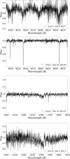 |
Fig. 1 Example of spectra of our target stars. Top: star 6 in Grus II, a hot HB star whose spectrum is dominated by Paschen lines. Middle: the Ca II triplet (2nd panel) and the CH band (3rd panel) spectra of the RGB star 26 in Grus II. Bottom: CH band spectrum of the RGB star 4 in Grus II. |
3 Atmospheric parameters and stellar models
3.1 Effective temperature
To derive the effective temperatures, the following formula was used (Mucciarelli & Bellazzini 2020):
 (1)
(1)
with θ defined as:
![Mathematical equation: \theta=b_0+b_1C+b_2C^2+b_3\text{[Fe/H]}+b_4\text{[Fe/H]}^2+b_5\text{[Fe/H]}\,C ,](/articles/aa/full_html/2026/03/aa57629-25/aa57629-25-eq4.png) (2)
(2)
where b0...b5 are the parameters for giant stars from Mucciarelli et al. (2021) and C represents the colors (BP-RP)0, (BP-G)0, and (G-RP)0, obtained from the magnitudes in the G, BP, and RP bands provided by Gaia. This calibration is not adequate for hot stars (Teff > 6500 K) since Eq. (2) holds for RGB stars, but it was used in this work with the sole aim of identifying the HB stars. The spectra were then confirmed as belonging to hot stars by checking for the presence of strong Paschen lines (see Fig. 1, top panel). Moreover, we compared the position of the stars in the color-magnitude diagram (Figs. 2 and A.1) with our results to confirm a reliable identification of HB stars, all having (BP-RP) ≲ 0.5. The colors are extinction and reddening corrected; the extinction factor is
 (3)
(3)
where X are the magnitudes (G, BP, RP) and kx is defined by Eq. (1) of Gaia Collaboration (2018). The color-independent extinction coefficient is provided by Gaia : A0 = 3.1 E (B -V), where E(B - V) is the color excess. The term (BP-RP)0 that appears in the definition of kX was derived by performing four iterations, with (BP-RP)0 equal to (BP-RP) and measured directly by Gaia as the initial guess. The results were used to derive the AX coefficients and, therefore, the real magnitudes and colors.
The final adopted Teff is the average of the three Teff obtained from the three colors. Tables E.2 and E.3 report the corrected colors and the mean effective temperature of every star of the sample. The error on the Teff is
 (4)
(4)
where  is the error on the mean of the three color temperatures, while
  is the mean of the three errors associated with the colors (s1 = 83 K, s2 = 83 K, and s3 = 71 K), which represents the intrinsic systematic error of the estimated method from Mucciarelli et al. (2021).
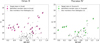 |
Fig. 2 Color-magnitude diagram of Grus II (left panel) and Tucana IV (right panel). The star symbols indicate our FLAMES-GIRAFFE targets, larger symbols are the member stars determined in Sect. 4.1, and small black circles represent possible members from the catalog by Battaglia et al. (2022) based on Gaia eDR3 measurements. Numbers are the star IDs (Table E.2 and Table E.3). Figure A.1 also shows the CMD with isochrones of different metallicities overplotted. |
3.2 Surface gravity
The surface gravity was evaluated using the known Stefan-Boltzmann relation (see, e.g., Skúladóttir et al. 2024):
 (1)
(1)
where Mbol,* = G0 - (m - M) + BC is the bolometric magnitude and BC is the bolometric correction (derived using Eq. (7) in Andrae et al. 2018). The stellar mass considered is the typical one of the RGB stars in UFDs, i.e., 0.8 ± 0.2 M⊙. The solar values used are log g⊙ = 4.44, Teff,⊙ = 5772 K, and Mbol,⊙ = 4.74. The error on the log g* was found assuming negligible errors on the solar parameters:
 (6)
(6)
3.3 Microturbulence velocity
From Anthony-Twarog et al. (2013), we used the empirical relation
 (7)
(7)
The error on the vturb was found with
 (8)
(8)
where  km s−1, which represents the average scatter between the empirical relation and the measurements (Carretta et al. 2004).
3.4 Stellar models and synthetic spectra
Synthetic spectra were generated using a grid of model atmospheres with a radiative and convective scheme (MARCS; Gustafsson et al. 2008) combined with Turbospectrum (Plez 2012). The grid of MARCS 1D atmosphere models was downloaded with the “standard composition”, that is, including the classical α enhancement of +0.4 dex at low metallicity, from the MARCS website2 (Gustafsson et al. 2008) and interpolated using Thomas Masseron’s interpol_modeles code for the given parameters of each star. Synthetic spectra were computed for each model, starting from solar chemical-abundance ratios ([X/Fe]=0) and an estimated metallicity of -2.0. This first estimate of [Fe/H] is used to generate the synthetic spectrum for the derivation of the radial velocity, which is not sensitive to the exact assumed [Fe/H]. Employing the χ2 minimization method, we find the best fit to an observed spectrum to derive the radial velocities (Sect. 4.1) and chemical abundances (Sect. 5).
4 Membership determination
4.1 Radial velocities
After carrying out an accurate continuum-level identification that allowed us to normalize the stellar spectra, our aim was to determine the members among the target stars. We derived the radial velocity (vrad) from the Ca II triplet lines using the minimization of the χ2 method. This was done by comparing the observed spectrum with synthetic spectrum, assuming different values of vrad in steps of 0.1 km s−1 in a range of ±100 km s−1 around the average of the galaxies (McConnachie 2012). The best fit to a synthetic spectrum (created by adopting the stellar parameters calculated in Sect. 3) determined the final vrad (see Fig. 3). Figure 4 shows radial-velocity distributions of Grus II and Tucana IV derived from the red spectra.
The radial velocities of every targeted star we analyzed in Grus II and Tucana IV are listed in Table E.1 with corresponding uncertainties. Two stars (2 and 19) in Grus II were discarded from our analysis since their S/N was very low, preventing us from obtaining reliable measurements. Stars 1, 14, and 114 in Grus II and star 125 in Tucana IV do not have any available exposures in the red setting; therefore, their radial velocities are only derived from the blue LR2 setting.
The errors on the radial velocity were found by performing Monte Carlo simulations. Using a template spectrum, we made 1000 iterations by adding random Gaussian noise to obtain mock observed spectra at five fixed S/Ns (5, 15, 30, 50, and 70 pix−1 ). After defining an array of radial velocity in steps of 0.1 km s−1, the best value of vrad was found for all the Monte Carlo spectra, comparing them with the best synthetic spectra of the stars in the sample. The distribution of the best values should be centered around zero, but the dispersion increases with lower S/N. Additionally, we tested this method using spectra with different stellar parameters and obtained consistent results. The sigma of the distributions derived for these five fixed S/N values serves as a reference for performing a polynomial fit to the curve of the radial velocity error as a function of the S/N (typically σvrad ≲ 0.4 km s−1 for S/N > 20 pix−1, σvrad ~ 1.5 km s−1 at S/N ~ 10 pix−1 and σvrad ~ 2.5 km s−1 at S/N ~ 5 pix−1). Moreover, star 22 in Grus II is a special case since the Ca triplet lines are completely contaminated by the sky lines; we derived the radial velocities of the two exposures using the Paschen line at ~8600Å. Since this is a broad line, we expected large uncertainty and indeed obtained an error of 5 km s−1 by visual inspection of the comparison between the observed and template spectra. Two separate polynomial fits were done for the RGB and HB member stars, since the spectra have different features (Fig. 1).
Additionally, we derived the vrad from the CH-band region for all the stars with LR2 spectra, obtaining the same member identification given by the red spectra. However, these measurements are less reliable since the spectra are of lower resolution (see Table 1), the S/N is typically lower than the red spectra, and the CH band contains many broad molecular features. Moreover, the radial velocity from broad lines, Hδ, and Hγ are less trustworthy than the ones obtained with the Ca II triplet. Furthermore, while the wavelength calibration in HR21 was checked by the positions of the location of the sky lines, there are no sky lines available in the blue LR2 region. This is why the preferred procedure involves the narrower atomic lines of the Ca II triplet. The same procedure was used for the errors in the blue region as for the red region. However, since there are no skylines, the zero point could not be verified, and therefore the systematic errors are not included in the estimated uncertainties. Figure C.1 compares the results of the radial velocity derived from the red and blue spectra.
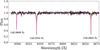 |
Fig. 3 Ca II triplet of star 26 in Grus II. The black line shows the observed spectrum, and the magenta line shows the synthetic spectrum best fit to the radial velocity of the star. |
4.2 Combining radial velocities with Gaia
For the final member identification, we combined our measured radial velocities with information from Gaia. In Fig. 5, we report the histograms of the membership probability of our stars according to Battaglia et al. (2022). The colored bars represent the identified member stars, while the gray bars show the nonmembers. Figure 6 shows the proper motion in RA and Dec of the stars color-coded by the probability of membership (updated to include information of the vrad measurements) and the average systemic proper motion of the galaxy from Battaglia et al. (2022). Figure 7 shows the positions of the stars color-coded by the radial velocity derived in Sect. 4.1. All these results are discussed in detail in the following subsections.
4.2.1 Grus II
Since the radial-velocity distribution of Grus II shows a large velocity offset with respect to Milky Way stars (see Fig. 4), the 11 members we identified in Grus II are clearly separated from the non-members. The systemic radial velocity of the galaxy was obtained by calculating the weighted mean of the radial velocity of the individual member stars, vsys = -106.3 ± 0.1 km s−1, while the velocity dispersion is σ = 4.7 ± 1.0 km s−1. After the derivation of radial velocity and establishment of the star members belonging to the galaxies, we compared our results with the membership probability based on Gaia eDR3 only, reported in Battaglia et al. (2022); see our Fig. 5. According to this catalog, all of the Grus II star members we found have a probability of belonging to the galaxy higher than 80%. The non-member stars, on the other hand, exhibit a probability lower than 60%, (Fig. 5). We note that the HB star 22 shows some signature of variability in radial velocity (see Appendix C).
We note that stars 1, 14, and 114 (all HB stars) only have blue spectra available (see Sect. 4.1). Therefore, we derived the radial velocities from the CH-band: the values are vrad = -98.8 ± 0.5 km s−1, vrad = -104.0 ± 1.2 km s−1, and vrad = -22.4 ± 1.9 km s−1, respectively. The proper motions of stars 1 and 14 (μαcos(δ) = 0.273 ± 0.221 and μδ = -1.624 ± 0.213 and μαcos(δ) = 0.496 ± 0.195 and μδ = -1.527 ± 0.198, respectively) and their position on the CMD (Fig. 2) support their identification as members, while star 114 is classified as a non-member since its radial velocity differs by >5σ from the peak of the distribution. Therefore, we confirmed 13 stars as Grus II members in total. However, to ensure the self-consistency of our results, we do not include these stars (with only blue spectra) in Figs. 4 and 6 or in the following analysis. The proper motions of the member stars of Grus II are shown in Fig. 6 and they are all consistent with the systemic proper motions. Moreover, we do not see any velocity gradient that indicates a tidal disruption of the galaxy (see Fig. 7).
4.2.2 Tucana IV
The mean radial velocity of Tucana IV is relatively close to zero (see Fig. 4), leading to similar radial velocity between members and non-members due to Galactic contamination. Moreover, we do not know the impact of binary stars; therefore, we did not exclude a priori the stars that differ less than 3σ from the center of the distribution (stars 9, 16, 17, 22, and 113), where σ is the standard deviation of the distribution considering the certain and potential members identified in this part of the analysis. We found 12 stars within 50 km s−1 from the average radial velocity of Tucana IV. Here, we performed a very broad membership assignment based only on the radial-velocity information with the aim of not excluding potential members in binary systems. This will now be refined to include also the probabilities of membership determined from Gaia, since we are aware that not all of the considered stars are binaries. Star 125 only has blue LR2 exposures available, from which we obtain vrad = -40.0 ± 2.5 km s−1; this likely makes it a non-member (corroborated by its position on the CMD; see Fig. 2). As previously mentioned, we do not include this star in further discussion to ensure self-consistency.
In the case of Tucana IV, we re-derived the membership probability adding the information of the radial velocity and the corresponding errors obtained in this work, following the approach explained in detail in Battaglia et al. (2022). This is shown in Fig. 6. The stars that fall in the main peak of the radialvelocity distribution have a probability of ~99% of being members. We paid particular attention to five stars that have a radial velocity that differs by more than 2σ from the average: stars 9, 16, 17, 22, and 113. According to the Battaglia et al. (2022) method, these stars have a very low probability of being members. Furthermore, considering in particular their offset in radial velocity, we can conclude that these five stars are “unlikely members,” as we do not expect all of them to be binaries. However, since the Gaia CMD and astrometry are moderately reasonable (see Fig. 2 and Fig. 6), we still analyze them in Appendix B. The systemic radial velocity of Tucana IV is vsys = 16.2 ± 0.2 km s−1, and the velocity dispersion is σ = 5.1 ± 1.3 km s−1. Finally, in checking the position of the member and potential member stars color-coded by the radial velocity (Fig. 7), we do not see any signatures of tidal disruption in this UFD.
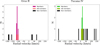 |
Fig. 4 Radial-velocity distribution of Grus II (left panel) and Tucana IV (right panel). The black bars represent the non-members, and the colored ones show the members. The shaded bars represent the HB members, which do not present any significant difference or offset from the RGB stars in radial velocity. We only include stars with red spectra available, but we note that the HB stars 1 and 14 in Grus II are members based only on measurements from blue spectra (Table E.1). |
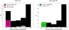 |
Fig. 5 Histograms of membership probability in Grus II and Tucana IV from Battaglia et al. (2022), showing our targets in colors (members) and in gray (our non-members). We note that non-member stars 10, 16, 23, 121 in Grus II and 3, 13, 15, 23 in Tucana IV are not included in the Battaglia et al. (2022) catalog. |
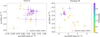 |
Fig. 6 Proper motions of stars in Grus II and Tucana IV from Gaia DR3. The stars are color-coded according to the membership probability based on Battaglia et al. (2022), updated to include the vrad measured here. The red cross shows the systemic proper motion (Battaglia et al. 2022); the red ellipse corresponds to 1σ, which is the error on the mean proper motions. |
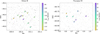 |
Fig. 7 Positions of our member stars color-coded by radial velocity. |
5 Chemical abundance analysis
We performed this analysis for RGB star member candidates from Sect. 4.1 both for metallicities and [C/Fe] abundances (see Table 2). We adopted the solar reference values from Asplund et al. (2009). The chemical abundances of the “unlikely members” of Tucana IV are listed in Table B.1. However, if they are not members, the adopted stellar parameters are probably not reliable.
5.1 Iron
We derived the [Fe/H] ratios using the second and third EWs of the Ca II triplet lines (8542 Å and 8662 Å) through the empirical relation of Starkenburg et al. (2010, their Eq. (5)). We used these lines because the S/N is not sufficient to accurately measure the metallicity from the weak Fe lines in these metal-poor stars. We converted our G Gaia magnitude to V Johnson-Cousin magnitude using the following formula (Carrasco & Bellazzini 2020):

The synthetic spectrum of all Ca II triplet lines was created using Turbospectrum in a well-defined smaller wavelength range (as explained in Sect. 3.4). In this case, it was not possible to gain accurate fits with 1D LTE synthetic spectra with correct parameters due to nonlocal thermodynamic equilibrium (NLTE) effects, which affect the line profile in a way that is not reproduced with the LTE synthetic spectra, but can be mimicked by changing the input parameters. The EWs were then measured from the best-fit synthetic spectrum, minimizing the χ2 (Fig. 8).
Tolstoy et al. (2023) reported the ratio between the EWs of the second and third lines of the calcium triplet as a function of S/N for RGB stars in the Sculptor dSph galaxy. To verify that our results are not skewed in the limit of the lowest S/N, Fig. 9 shows the comparison of our measured EW ratio, EW2/EW3, with their results. Since we have no measurements in the region beyond that considered reasonable by Tolstoy et al. (2023), we infer that the EW ratios are constant with the S/N as expected, indicating that our results are not severely skewed in the limit of a low S/N. In the right panel of Fig. 9, we highlight the difference between the reddest Ca II triplet line (8662 Å) for a metal-poor and a metal-rich star.
Figure 10 shows the metallicity distribution function (MDF) of the member stars in Grus II and Tucana IV. The MDF of Grus II is shifted toward lower metallicity than that of Tucana IV, leading to a higher probability of finding CEMP-no stars in the first galaxy since these stars are more common at low metallicity (e.g., Beers & Christlieb 2005; Salvadori et al. 2015). Because of the low number statistics (especially in Tucana IV), we cannot draw any concrete conclusion regarding the star formation history.
According to Starkenburg’s formula, the errors on [Fe/H] are obtained with
![Mathematical equation: \sigma_{[\mathrm{Fe/H}]} =\sqrt{%\begin{aligned}[t]& (0.195 + 0.0155 EW_{2+3})^{2}\,\sigma_{V - V_{\mathrm{HB}}}^{2} + (0.458 + \\ &1.3695EW_{2+3}^{-2.5} + 0.0155(V - V_{\mathrm{HB}}))^{2}\,\sigma_{EW_{2+3}}^{2} + \sigma_{\rm par}^2\end{aligned}%,}](/articles/aa/full_html/2026/03/aa57629-25/aa57629-25-eq15.png) (9)
(9)
where σEW2+3 is the error on the sum of EW2 and EW3; σ(v-vHB) is the error on the mean of the V magnitude of HB stars (VHB=19.14 ± 0.14 for Grus II and VHB=19.07 ± 0.14 for Tucana IV, derived by averaging the V magnitude of the HB stars in our sample); and σpar is the contribution derived from the fit parameters, estimated to be 8% (Starkenburg et al. 2010). The error on the individual EWs is found by adopting the formula from Battaglia et al. (2008, their Eq. (3)) and then summed in quadrature. The [Fe/H] values of member stars and their respective errors are reported in Table 2. Moreover, we tested the impact of the systematic error due to the continuum level assuming different S/N, which results in ![Mathematical equation: $\sigma_{\rm [Fe/H],sys}\lesssim$ 0.05](/articles/aa/full_html/2026/03/aa57629-25/aa57629-25-eq16.png) .
.
We checked for the brightest stars (five in Tuc IV and 26 in Grus II) measuring the [Fe/H] with the Fe lines, and the results are in agreement with the Ca triplet measurements.
Chemical measurements of RGB member stars in Grus II and Tucana IV.
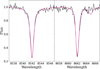 |
Fig. 8 Best fit of EW2 (8542 Å) and EW3 (8662 Å) of star 26 in Grus II. The black line shows the observed spectrum, the magenta line is the synthetic spectrum. |
5.2 Carbon
To measure the C abundances (Fig. 1), we created a synthetic spectrum as described in Sect. 4.1, adopting the stellar parameters from Sect. 3 and [Fe/H] from Sect. 5.1. The synthetic spectrum was generated around the CH-band at 4300 Å in a wavelength range of 80 Å (Fig. 11). We used the online tool developed by Placco et al. (2014) to correct the C abundances for the internal mixing occurring in the RGB stars.
Figure 12 shows the [C/Fe] relation as a function of [Fe/H]. In Grus II, we identify three CEMP stars (stars 4, 9, and 30) with [C/Fe] > +1 and 2 CEMP stars (stars 13 and 29) with [C/Fe] > +0.7 and slightly higher [Fe/H]. In Tucana IV, star 7 has [C/Fe] > +0.7. All the C measurements are reported in Table 2.
For these CEMP stars, we looked at the Ba II line at 4554 Å in LR2. However, since the line is at the edge of the spectrum and the S/N is very low (Table E.1), we were only able to derive upper limits of the Ba abundances: in Grus II, stars 4 and 13 have [Ba/Fe] ≲ 0.6, star 29 has [Ba/Fe] ≲ 0.2, and stars 30 and 9 have [Ba/Fe] ≲ 0.7. In Tucana IV, star 7 has [Ba/Fe] ≲ 0.2. Additionally, we derived the absolute abundances A(C) to verify the nature of these CEMP stars (Fig. 12, right); we point out that the stars that fall in the high-C band (i.e., have an absolute C abundance close to the solar value) populate a region that is primarily occupied by CEMP-s stars (Bonifacio et al. 2015). Remembering that CEMP-s stars have [Ba/Fe] > 1 and high absolute C abundances, we can conclude that all the CEMP stars found in Grus II and star 7 in Tucana IV are CEMP-no stars. We note that technically these identified CEMP stars could be CEMP-r stars since we do not have Eu measurements. However, this kind of CEMP star is extremely rare, and only a few have been identified in the Milky Way halo.
All the abundances (Fe, C, and Ba) were derived under the LTE assumption, allowing us to compare the abundances with other measurements present in the literature. The uncertainties on the C abundances consist of two contributions, which were added quadratically to obtain the total errors. The first is the random error, which was found by deriving the [C/Fe] in five different regions of 10 Å from 4270 Å to 4320 Å, covering the entire CH band. We obtained the errors by calculating the standard deviation of these five [C/Fe] measurements. For S/N > 7, σC,rand is ≲ 0.1 dex, while for 5 < S/N < 7, σC,rand is ~ 0.15 dex3. The second contribution is due to the stellar parameters and is dominated by the error on the Teff, i.e., σC,Teff ~ 0.2 dex. The total error on [C/Fe] was found with the quadratic sum of both the errors on C and Fe abundances (see Table 2).
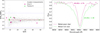 |
Fig. 9 Left : EW ratios of two Ca II lines (8542 Å and 8662 Å) as a function of S/N. The two horizontal blue lines are limits of EW2/EW3 at 0.2<EW2∕EW3<2.2, defined as reasonable values by Tolstoy et al. (2023). Right : comparison between spectra of the metal-rich star 5 in Tucana IV and the metal-poor star 26 in Grus II. |
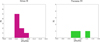 |
Fig. 10 Metallicity distribution functions. In Tucana IV, the “unlikely members” are not included in the distribution. The typical errors on the [Fe/H] are 0.27. |
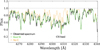 |
Fig. 11 Best fit of the CH band of star 5 in Tucana IV. The black line shows the observed spectrum, and the green line shows the synthetic spectrum. |
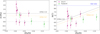 |
Fig. 12 Left : [C/Fe] as a function of metallicity. The dashed orange line is [C/Fe] = +0.7, while the black dashed line is the other threshold commonly assumed in the literature for CEMP stars, [C/Fe] = +1. Right : The absolute C abundance as a function of [Fe/H]. The dashed blue line represents the solar value A(C)⊙ = 8.43 (Asplund et al. 2009). |
6 Comparison with literature
Both Grus II and Tucana IV were also investigated by Simon et al. (2020). The authors observed stars in Grus II and Tucana IV with the IMACS spectrograph on the Magellan/Baade Telescope. Their spectra had R=11 000 in a wavelength range from 7500 to 8900 Å. We checked the presence of stars in common between the two samples: there are 14 stars in Grus II and nine stars in Tucana IV in common, allowing us to compare the results. The upper panels of Fig. 13 show the comparison between the radial-velocity distributions, while the number values are reported in Tables E.4 and E.5. The darker gray bars show the members identified by Simon et al. (2020); our distributions are completely in agreement, corroborating our identification of the members. We remind the reader that the systemic radial velocity we derived for Grus II is vsys = -106.5 ± 1.4 km s−1, resulting in a small offset from the value reported by Simon et al. (2020): vsys = -110.0 ± 0.5 km s−1. In the case of Tucana IV, the systemic radial velocity is vsys = 14.9 ± 1.9 km s−1, which is in good agreement with the value from Simon et al. (2020): vsys = 15.9 km s−1.
Additionally, we compared the metallicity distribution functions with those of Simon et al. (2020). The [Fe/H] measurements of stars in common are consistent within the errors; therefore, despite the low number of stars, the two distributions are in agreement (see the lower panels in Fig. 13). Numerical values are reported in Tables E.4 and E.5.
Finally, Hansen et al. (2020) analyzed the three brightest stars in Grus II (3, 26, 122) from a detailed chemical point of view, also providing the radial velocities (which are in agreement with our results). For the purpose of this work, our attention is focused on the C abundance. All the [Fe/H] measurements and the [C/Fe] of stars 26 and 122 are consistent, while star 3 has quite a different [C/Fe]; however, we agree on it being a C-normal star (see Appendix D). Nevertheless, it is not a CEMP star, as we confirm with our abundance derivation.
7 Discussion and conclusions
The aim of this work was to analyze the spectra of stars that belong to two ultra-faint dwarf galaxies, Grus II and Tucana IV, and derive the carbon abundance in RGB members. In particular, we focused on identifying the CEMP-no stars, whose chemical abundances are consistent with the imprint of primordial low-energy supernovae (E ≲ 1051 erg).
We derived the radial velocity of RGB and HB stars (Fig. 4) using the Ca II triplet from the FLAMES-Giraffe HR21 spectra and, hence, determined the membership of the stars to the galaxies by combining our results with Gaia data. Moreover, we compared our results by checking the membership probability reported in Battaglia et al. (2022) based on Gaia eDR3 (Fig. 6), where all of our identified members of Grus II have a membership probability higher than 80%. We note that two of the 13 Grus II members (stars 1 and 14) are HB stars with only LR2 spectra available; therefore, they are not present in the figures and the consequent analysis. In Tucana IV, there are seven members with a probability over 80%. Afterward, we derived the metallicity distribution functions of the galaxies after an accurate determination of the EWs of the Ca II triplet. Tucana IV was shifted to higher metallicity than Grus II (Fig. 10); therefore, the probability of finding CEMP stars is lower.
Finally, we derived the [C/Fe] to identify carbon-rich stars (Fig. 12); five CEMP-no stars (three of which have [C/Fe] > +1) were found in Grus II, while in Tucana IV we discovered one CEMP-no star. The categorization of CEMP-no stars was based on A(C) and upper limits on Ba (Sect. 5.2), but further investigation is needed to obtain reliable Ba measurements. Among our identified members in Grus II and Tucana IV, ten stars are very metal poor ([Fe/H]<-2); six of them are CEMP-no stars with [C/Fe] > +0.7. According to Ji et al. (2020), the fraction of CEMP stars at this metallicity is 21 ± 5%. In our case, this fraction is 60 (Gehrels 1986); thus, in these two UFDs the fraction of CEMP-no stars is higher than the average. Considering the threshold of [C/Fe] > +1, we found three CEMP-no stars, i.e., 30
 (Gehrels 1986), which is in agreement with the Ji et al. (2020) result of ≈10 ± 5% (assuming similar errors as for [C/Fe] > +0.7). We can conclude that in Grus II and Tucana IV, faint Pop III SNe likely exploded, enhancing the ISM with high [C/Fe] and maintaining this peculiar abundance ratio in the photosphere of the second-generation stars. However, in the case of Grus II (where we found five CEMP-no stars), we cannot conclude if these stars were derived from the same first faint SN or if several such events occured even in this small galaxy (M*=3.4
 ). Combining this data analysis with literature data could be potentially useful to constrain and understand the star formation history in these small systems.
Even though the UFDs are among the nearest galaxies in which it is possible to detect single stars, obtaining spectra of stars in these systems is challenging. This is why there are very few chemical measurements of the populations of these systems in the literature, contained in two principal catalogs: SAGA (Suda et al. 2008) and JINA (Abohalima & Frebel 2018). In the SAGA database, which contains the most complete compilation of literature C measurements in metal-poor stars, there are only 78 measurements of carbon abundances in UFDs. By only analyzing a few RGB stars in Grus II and Tucana IV, we improved this number by ~14%. This allowed us to better understand the CEMP fraction in the UFDs and the imprint that the first stars made on such pristine and ancient systems.
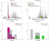 |
Fig. 13 Our radial velocity distributions (upper panels) and metallicity distribution functions (lower panels) compared with Simon et al. (2020). |
Acknowledgements
This project has received funding from the European Research Council (ERC) under the European Union’s Horizon 2020 research and innovation programme (grant agreement No. 101117455). J.M. Arroyo acknowledges support from the Agencia Estatal de Investigación del Ministerio de Ciencia en Innovación (AEI-MICIN) and the European Social Fund (ESF+) under grant PRE2021-100638. J.M. Arroyo and G. Battaglia acknowledge support from the Agencia Estatal de Investigación del Ministerio de Ciencia, Innovación y Universidades (MCIU/AEI) under grant “En La Frontera De La Arqueología Galáctica: Evolución De La Materia Luminosa Y Oscura De La Vía Láctea Y Las Galaxias Enanas Del Grupo Local En La Era De Gaia. (FOGALERA)” and the European Regional Development Fund (ERDF) with reference PID2023-150319NB-C21/10.13039/501100011033. A.Mucciarelli, acknowledges support from the project “LEGO - Reconstructing the building blocks of the Galaxy by chemical tagging” (PI: A. Mucciarelli) granted by the Italian MUR through contract PRIN 2022LLP8TK_001. D.Massari acknowledges financial support from PRIN-MIUR-22: CHRONOS: adjusting the clock(s) to unveil the CHRONOchemo-dynamical Structure of the Galaxy (PI: S. Cassisi), and from the “INAF Mini Grant z2023 (Ob.Fu. 1.05.23.04.02 - CUP C3 3C23000960005) CHAM -Chemo-dynamics of the Accreted Halo of the Milky Way (PI: M. Bellazzini). We thank J. Simon for useful discussion and insightful suggestions.
References
- Abohalima, A., & Frebel, A. 2018, ApJS, 238, 36 [NASA ADS] [CrossRef] [Google Scholar]
- Andrae, R., Fouesneau, M., Creevey, O., et al. 2018, A&A, 616, A8 [NASA ADS] [CrossRef] [EDP Sciences] [Google Scholar]
- Anthony-Twarog, B. J., Deliyannis, C. P., Rich, E., & Twarog, B. A. 2013, ApJ, 767, L19 [NASA ADS] [CrossRef] [Google Scholar]
- Aoki, W., Beers, T. C., Christlieb, N., et al. 2007, ApJ, 655, 492 [NASA ADS] [CrossRef] [Google Scholar]
- Asplund, M., Grevesse, N., Sauval, A. J., & Scott, P. 2009, ARA&A, 47, 481 [NASA ADS] [CrossRef] [Google Scholar]
- Battaglia, G., Irwin, M., Tolstoy, E., et al. 2008, MNRAS, 383, 183 [NASA ADS] [CrossRef] [MathSciNet] [Google Scholar]
- Battaglia, G., Taibi, S., Thomas, G. F., & Fritz, T. K. 2022, A&A, 657, A54 [NASA ADS] [CrossRef] [EDP Sciences] [Google Scholar]
- Beers, T. C., & Christlieb, N. 2005, ARA&A, 43, 531 [NASA ADS] [CrossRef] [Google Scholar]
- Bonifacio, P., Caffau, E., Spite, M., et al. 2015, A&A, 579, A28 [NASA ADS] [CrossRef] [EDP Sciences] [Google Scholar]
- Bovill, M. S., & Ricotti, M. 2009, ApJ, 693, 1859 [NASA ADS] [CrossRef] [Google Scholar]
- Bressan, A., Marigo, P., Girardi, L., et al. 2012, MNRAS, 427, 127 [NASA ADS] [CrossRef] [Google Scholar]
- Bromm, V., & Yoshida, N. 2011, ARA&A, 49, 373 [CrossRef] [Google Scholar]
- Brown, T. M., Tumlinson, J., Geha, M., et al. 2014, ApJ, 796, 91 [NASA ADS] [CrossRef] [Google Scholar]
- Carrasco, J. M., & Bellazzini, M. 2020, 5.5.1 Relationships with other photometric systems, https://gea.esac.esa.int/archive/documentation/GEDR3/, gaia EDR3 Documentation, ESA [Google Scholar]
- Carretta, E., Bragaglia, A., Gratton, R. G., & Tosi, M. 2004, A&A, 422, 951 [NASA ADS] [CrossRef] [EDP Sciences] [Google Scholar]
- Chiti, A., Simon, J. D., Frebel, A., et al. 2018, ApJ, 856, 142 [NASA ADS] [CrossRef] [Google Scholar]
- Chiti, A., Placco, V. M., Pace, A. B., et al. 2025, arXiv e-prints [arXiv:2508.04053] [Google Scholar]
- Drlica-Wagner, A., Bechtol, K., Rykoff, E. S., et al. 2015, ApJ, 813, 109 [Google Scholar]
- Frebel, A., & Bromm, V. 2012, ApJ, 759, 115 [Google Scholar]
- Frebel, A., Kirby, E. N., & Simon, J. D. 2010, Nature, 464, 72 [NASA ADS] [CrossRef] [Google Scholar]
- Gaia Collaboration (Babusiaux, C., et al.) 2018, A&A, 616, A10 [NASA ADS] [CrossRef] [EDP Sciences] [Google Scholar]
- Gallart, C., Monelli, M., Ruiz-Lara, T., et al. 2021, ApJ, 909, 192 [NASA ADS] [CrossRef] [Google Scholar]
- Gehrels, N. 1986, ApJ, 303, 336 [Google Scholar]
- Gustafsson, B., Edvardsson, B., Eriksson, K., et al. 2008, A&A, 486, 951 [NASA ADS] [CrossRef] [EDP Sciences] [Google Scholar]
- Hansen, T. T., Andersen, J., Nordström, B., et al. 2015, A&A, 583, A49 [NASA ADS] [CrossRef] [EDP Sciences] [Google Scholar]
- Hansen, T. T., Marshall, J. L., Simon, J. D., et al. 2020, ApJ, 897, 183 [Google Scholar]
- Hansen, T. T., Simon, J. D., Li, T. S., et al. 2024, ApJ, 968, 21 [NASA ADS] [CrossRef] [Google Scholar]
- Hartwig, T., & Yoshida, N. 2019, ApJ, 870, L3 [Google Scholar]
- Hirano, S., Hosokawa, T., Yoshida, N., et al. 2014, ApJ, 781, 60 [NASA ADS] [CrossRef] [Google Scholar]
- Iwamoto, N., Umeda, H., Tominaga, N., Nomoto, K., & Maeda, K. 2005, Science, 309, 451 [NASA ADS] [CrossRef] [Google Scholar]
- Jablonka, P., North, P., Mashonkina, L., et al. 2015, A&A, 583, A67 [NASA ADS] [CrossRef] [EDP Sciences] [Google Scholar]
- Jenkins, S. A., Li, T. S., Pace, A. B., et al. 2021, ApJ, 920, 92 [NASA ADS] [CrossRef] [Google Scholar]
- Jeon, M., Bromm, V., Besla, G., Yoon, J., & Choi, Y. 2021, MNRAS, 502, 1 [NASA ADS] [CrossRef] [Google Scholar]
- Ji, A. P., Li, T. S., Simon, J. D., et al. 2020, ApJ, 889, 27 [NASA ADS] [CrossRef] [Google Scholar]
- Koch, A., Hansen, T., Feltzing, S., & Wilkinson, M. I. 2014, ApJ, 780, 91 [Google Scholar]
- Komiya, Y., Suda, T., Yamada, S., & Fujimoto, M. Y. 2020, ApJ, 890, 66 [Google Scholar]
- Lee, Y. S., Beers, T. C., Masseron, T., et al. 2013, AJ, 146, 132 [Google Scholar]
- Lucchesi, R., Jablonka, P., Skúladóttir, Á., et al. 2024, A&A, 686, A266 [NASA ADS] [CrossRef] [EDP Sciences] [Google Scholar]
- Martínez-Vázquez, C. E., Vivas, A. K., Gurevich, M., et al. 2019, MNRAS, 490, 2183 [Google Scholar]
- Massari, D., & Helmi, A. 2018, A&A, 620, A155 [NASA ADS] [CrossRef] [EDP Sciences] [Google Scholar]
- McConnachie, A. W. 2012, AJ, 144, 4 [Google Scholar]
- Mucciarelli, A., & Bellazzini, M. 2020, RNAAS, 4, 52 [Google Scholar]
- Mucciarelli, A., Bellazzini, M., & Massari, D. 2021, A&A, 653, A90 [NASA ADS] [CrossRef] [EDP Sciences] [Google Scholar]
- Norris, J. E., Wyse, R. F. G., Gilmore, G., et al. 2010, ApJ, 723, 1632 [NASA ADS] [CrossRef] [Google Scholar]
- Norris, J. E., Yong, D., Bessell, M. S., et al. 2013, ApJ, 762, 28 [NASA ADS] [CrossRef] [Google Scholar]
- Pace, A. B., & Li, T. S. 2019, ApJ, 875, 77 [NASA ADS] [CrossRef] [Google Scholar]
- Placco, V. M., Frebel, A., Beers, T. C., & Stancliffe, R. J. 2014, ApJ, 797, 21 [Google Scholar]
- Plez, B. 2012, Turbospectrum: Code for spectral synthesis, Astrophysics Source Code Library [record ascl:1205.004] [Google Scholar]
- Rossi, M., Salvadori, S., & Skúladóttir, Á. 2021, MNRAS, 503, 6026 [NASA ADS] [CrossRef] [Google Scholar]
- Rossi, M., Salvadori, S., Skúladóttir, Á., Vanni, I., & Koutsouridou, I. 2024, Hidden Population III Descendants in Ultra-Faint Dwarf Galaxies [arXiv:2406.12960] [astro-ph] [Google Scholar]
- Salvadori, S., & Ferrara, A. 2009, MNRAS, 395, L6 [NASA ADS] [Google Scholar]
- Salvadori, S., Skúladóttir, Á., & Tolstoy, E. 2015, MNRAS, 454, 1320 [Google Scholar]
- Simon, J. D. 2019, ARA&A, 57, 375 [NASA ADS] [CrossRef] [Google Scholar]
- Simon, J. D., Jacobson, H. R., Frebel, A., et al. 2015, ApJ, 802, 93 [Google Scholar]
- Simon, J. D., Li, T. S., Erkal, D., et al. 2020, ApJ, 892, 137 [Google Scholar]
- Skúladóttir, Á., Tolstoy, E., Salvadori, S., et al. 2015, A&A, 574, A129 [NASA ADS] [CrossRef] [EDP Sciences] [Google Scholar]
- Skúladóttir, Á., Salvadori, S., Amarsi, A. M., et al. 2021, ApJ, 915, L30 [CrossRef] [Google Scholar]
- Skúladóttir, Á., Vanni, I., Salvadori, S., & Lucchesi, R. 2024, A&A, 681, A44 [NASA ADS] [CrossRef] [EDP Sciences] [Google Scholar]
- Starkenburg, E., Hill, V., Tolstoy, E., et al. 2010, A&A, 513, A34 [CrossRef] [EDP Sciences] [Google Scholar]
- Starkenburg, E., Hill, V., Tolstoy, E., et al. 2013, A&A, 549, A88 [NASA ADS] [CrossRef] [EDP Sciences] [Google Scholar]
- Starkenburg, E., Shetrone, M. D., McConnachie, A. W., & Venn, K. A. 2014, MNRAS, 441, 1217 [Google Scholar]
- Suda, T., Katsuta, Y., Yamada, S., et al. 2008, PASJ, 60, 1159 [NASA ADS] [Google Scholar]
- Susmitha, A., Koch, A., & Sivarani, T. 2017, A&A, 606, A112 [NASA ADS] [CrossRef] [EDP Sciences] [Google Scholar]
- Tafelmeyer, M., Jablonka, P., Hill, V., et al. 2010, A&A, 524, A58 [CrossRef] [EDP Sciences] [Google Scholar]
- Tegmark, M., Silk, J., Rees, M. J., et al. 1997, ApJ, 474, 1 [NASA ADS] [CrossRef] [Google Scholar]
- Tolstoy, E., Skúladóttir, Á., Battaglia, G., et al. 2023, A&A, 675, A49 [NASA ADS] [CrossRef] [EDP Sciences] [Google Scholar]
Appendix A Isochrones
Figure A.1 shows the CMD with isochrones from PARSEC tool (Bressan et al. 2012) plotted for different metallicity. We note that below G<20 we reach the limit of Gaia, so a spread in photometry is expected because of large uncertainties and our data are not deep enough to reach the main sequence turn-off. The HB of our data agrees with the isochrones, showing that we are in agreement with the distances estimated in Drlica-Wagner et al. (2015).
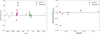 |
Fig. A.1 Color-magnitude diagram with isochrones. Our stars fall on the RGB and HB. |
Appendix B Radial velocity analysis of near-peak stars in Tucana IV
Radial velocity and chemical abundances of the stars 9, 16, 17, 22 and 113 in Tucana IV.
Stars 9, 16, 17, 22 and 113 in Tucana IV are classified as "unlikely members" according to radial velocity determination (Sect. 4.1) and Gaia parameters (proper motions, parallax and position on CMD). However, we performed the chemical abundance analysis described in Sect. 5 also for these stars and the results are reported in Table B.1.
We derived different radial velocities of star 16 from exposures obtained in different epochs (-19.2 km s−1 and -16.7 km s−1), which suggests a possible binary star. However, the deviation from the mean velocity of the galaxy is large so its semi-amplitude would be larger than that of binary systems already identified in dwarf galaxies (Koch et al. 2014; Hansen et al. 2024), making this star an unlikely member of Tucana IV. Star 22 is a possible CEMP-s star (i.e., likely a binary star; see Sect. 5.2) which can explain its deviation from the central peak. However, without certain [Ba/Fe] abundance measurements, we cannot confirm its nature. Moreover, the semi-amplitude would be too large for the star to be a Tucana IV member (as in the case of star 16). Stars 17 and 113 have acceptable proper motions and parallax, but we do not see any evidence of binarity due in part to having only two epochs. Star 9 differs 5σpm from the systemic proper motion of Tucana IV (see Fig. 6). Here, σpm denotes the total dispersion of the proper motions distribution.
Stars 16, 17 and 22 have [C/Fe] consistent with the threshold for CEMP classification. In particular, star 22 has [Ba/Fe] ≲ 1.5 and falls in the high-C band, therefore could be classified as a possible CEMP-s star. However, we note that should any of these stars be non-members at very different distances compared to the galaxies, the derived stellar abundances, and hence also their chemical abundance measurements, cannot be considered reliable.
Appendix C Radial velocity in blue
Figure C.1 shows the difference between the radial velocities measured from the HR21 and LR2 spectra. The solid line is the mean of the difference, while the dashed lines are ±1σ from the mean. We note that the zero-point in the blue could not be verified because of the lack of skylines, therefore the errors do not include a possible systematic offset. Stars 22 in Grus II and 12 in Tucana IV are HB stars and have very different radial velocities between red and blue. However, we remember that the blue spectra present very broad molecular features, lower S/N and resolution that make the radial velocity measurements less trustworthy than the ones from the Ca II triplet (see Sect. 4.1). For these stars, we also obtained the radial velocities from the two epochs available: for star 22 in Grus II we found ∆v =10 km s−1 and for star 12 in Tucana IV ∆v=2.5 km s−1, indicating that the hypothesis of binaries could not be excluded. In particular, star 22 in Grus II is a special case, since the Ca triplet lines are completely contaminated by the skylines as we explained in Sect. 4.1. Moreover, we note that this star corresponds to the variable star V2 studied in Martínez-Vázquez et al. (2019), who conclude that this is more likely to be a member of the Orphan-Chenab stellar stream. Thus, the radial velocity variation detected in star 22 in our Grus II sample is likely caused by pulsations.
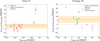 |
Fig. C.1 Difference of radial velocity measurements in the red and the blue. The solid line is the mean of the difference, the shaded areas cover ±1σ from the mean. Left: Star 22 shows a big offset, which can indicate a possible binary nature and/or be a sign of pulsations. Right: Stars 9, 16, 17, 22, and 113 are classified as "unlikely members," as explained in Sect. 4.2. |
Appendix D Comparison with literature results
In Table D.1 are listed the three stars in Grus II in common with Hansen et al. (2020). The radial velocities are in agreement within the errors for all the stars. Moreover, the metallicities and carbon abundances are consistent with Hansen et al. (2020) within the errors.
Comparison with (Hansen et al. 2020) for the three stars in common.
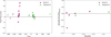 |
Fig. D.1 Comparison between our and Simon et al. (2020) results in radial velocity (left) and [Fe/H] (right). The empty symbols are the nonmember stars. |
Appendix E Additional tables
Number of exposures in HR21 and LR2 settings with the corresponding S/N per pixel values, and radial velocities from the Ca triplet with corresponding uncertainties.
Stellar parameters and Gaia DR3 data for Grus II.
Stellar parameters and Gaia DR3 data for Tucana IV.
Comparison between stars of Grus II in our sample and Simon et al. (2020).
Comparison between stars of Tucana IV in our sample and Simon et al. (2020).
We remind the reader that the S/N was underestimated in the region of the CH band because of the lack of continuum points available (see Sect. 2).
All Tables
Radial velocity and chemical abundances of the stars 9, 16, 17, 22 and 113 in Tucana IV.
Number of exposures in HR21 and LR2 settings with the corresponding S/N per pixel values, and radial velocities from the Ca triplet with corresponding uncertainties.
All Figures
|
Fig. 1 Example of spectra of our target stars. Top: star 6 in Grus II, a hot HB star whose spectrum is dominated by Paschen lines. Middle: the Ca II triplet (2nd panel) and the CH band (3rd panel) spectra of the RGB star 26 in Grus II. Bottom: CH band spectrum of the RGB star 4 in Grus II. |
| In the text | |
|
Fig. 2 Color-magnitude diagram of Grus II (left panel) and Tucana IV (right panel). The star symbols indicate our FLAMES-GIRAFFE targets, larger symbols are the member stars determined in Sect. 4.1, and small black circles represent possible members from the catalog by Battaglia et al. (2022) based on Gaia eDR3 measurements. Numbers are the star IDs (Table E.2 and Table E.3). Figure A.1 also shows the CMD with isochrones of different metallicities overplotted. |
| In the text | |
|
Fig. 3 Ca II triplet of star 26 in Grus II. The black line shows the observed spectrum, and the magenta line shows the synthetic spectrum best fit to the radial velocity of the star. |
| In the text | |
|
Fig. 4 Radial-velocity distribution of Grus II (left panel) and Tucana IV (right panel). The black bars represent the non-members, and the colored ones show the members. The shaded bars represent the HB members, which do not present any significant difference or offset from the RGB stars in radial velocity. We only include stars with red spectra available, but we note that the HB stars 1 and 14 in Grus II are members based only on measurements from blue spectra (Table E.1). |
| In the text | |
|
Fig. 5 Histograms of membership probability in Grus II and Tucana IV from Battaglia et al. (2022), showing our targets in colors (members) and in gray (our non-members). We note that non-member stars 10, 16, 23, 121 in Grus II and 3, 13, 15, 23 in Tucana IV are not included in the Battaglia et al. (2022) catalog. |
| In the text | |
|
Fig. 6 Proper motions of stars in Grus II and Tucana IV from Gaia DR3. The stars are color-coded according to the membership probability based on Battaglia et al. (2022), updated to include the vrad measured here. The red cross shows the systemic proper motion (Battaglia et al. 2022); the red ellipse corresponds to 1σ, which is the error on the mean proper motions. |
| In the text | |
|
Fig. 7 Positions of our member stars color-coded by radial velocity. |
| In the text | |
|
Fig. 8 Best fit of EW2 (8542 Å) and EW3 (8662 Å) of star 26 in Grus II. The black line shows the observed spectrum, the magenta line is the synthetic spectrum. |
| In the text | |
|
Fig. 9 Left : EW ratios of two Ca II lines (8542 Å and 8662 Å) as a function of S/N. The two horizontal blue lines are limits of EW2/EW3 at 0.2<EW2∕EW3<2.2, defined as reasonable values by Tolstoy et al. (2023). Right : comparison between spectra of the metal-rich star 5 in Tucana IV and the metal-poor star 26 in Grus II. |
| In the text | |
|
Fig. 10 Metallicity distribution functions. In Tucana IV, the “unlikely members” are not included in the distribution. The typical errors on the [Fe/H] are 0.27. |
| In the text | |
|
Fig. 11 Best fit of the CH band of star 5 in Tucana IV. The black line shows the observed spectrum, and the green line shows the synthetic spectrum. |
| In the text | |
|
Fig. 12 Left : [C/Fe] as a function of metallicity. The dashed orange line is [C/Fe] = +0.7, while the black dashed line is the other threshold commonly assumed in the literature for CEMP stars, [C/Fe] = +1. Right : The absolute C abundance as a function of [Fe/H]. The dashed blue line represents the solar value A(C)⊙ = 8.43 (Asplund et al. 2009). |
| In the text | |
|
Fig. 13 Our radial velocity distributions (upper panels) and metallicity distribution functions (lower panels) compared with Simon et al. (2020). |
| In the text | |
|
Fig. A.1 Color-magnitude diagram with isochrones. Our stars fall on the RGB and HB. |
| In the text | |
|
Fig. C.1 Difference of radial velocity measurements in the red and the blue. The solid line is the mean of the difference, the shaded areas cover ±1σ from the mean. Left: Star 22 shows a big offset, which can indicate a possible binary nature and/or be a sign of pulsations. Right: Stars 9, 16, 17, 22, and 113 are classified as "unlikely members," as explained in Sect. 4.2. |
| In the text | |
|
Fig. D.1 Comparison between our and Simon et al. (2020) results in radial velocity (left) and [Fe/H] (right). The empty symbols are the nonmember stars. |
| In the text | |
Current usage metrics show cumulative count of Article Views (full-text article views including HTML views, PDF and ePub downloads, according to the available data) and Abstracts Views on Vision4Press platform.
Data correspond to usage on the plateform after 2015. The current usage metrics is available 48-96 hours after online publication and is updated daily on week days.
Initial download of the metrics may take a while.