| Issue |
A&A
Volume 707, March 2026
|
|
|---|---|---|
| Article Number | A38 | |
| Number of page(s) | 10 | |
| Section | Galactic structure, stellar clusters and populations | |
| DOI | https://doi.org/10.1051/0004-6361/202557817 | |
| Published online | 03 March 2026 | |
Optically thick winds of very massive stars suppress intermediate-mass black hole formation
1
Max-Planck-Institut für Astronomie,
Königstuhl 17,
69117
Heidelberg,
Germany
2
Universität Heidelberg, Zentrum für Astronomie (ZAH), Institut für Theoretische Astrophysik,
Albert Ueberle Str. 2,
69120
Heidelberg,
Germany
3
Universität Heidelberg, Interdiszipliäres Zentrum für Wissenschaftliches Rechnen,
69120
Heidelberg,
Germany
4
Dipartimento di Fisica e Astronomia Galileo Galilei, Università di Padova,
Vicolo dell’Osservatorio 3,
35122
Padova,
Italy
5
INFN, Sezione di Padova,
Via Marzolo 8,
35131
Padova,
Italy
6
Gran Sasso Science Institute (GSSI),
Viale Francesco Crispi 7,
67100
L’Aquila,
Italy
7
INFN, Laboratori Nazionali del Gran Sasso,
67100
Assergi,
Italy
8
Departament de Física Quàntica i Astrofísica, Institut de Ciències del Cosmos, Universitat de Barcelona,
Martí i Franquès 1,
08028
Barcelona,
Spain
★ Corresponding authors: This email address is being protected from spambots. You need JavaScript enabled to view it.
; This email address is being protected from spambots. You need JavaScript enabled to view it.
; This email address is being protected from spambots. You need JavaScript enabled to view it.
Received:
24
October
2025
Accepted:
19
December
2025
Abstract
Intermediate-mass black holes (IMBHs) are the link between stellar-mass and supermassive black holes. Gravitational waves have started to unveil a population of IMBHs in the ~100–300 M⊙ range. Here, we investigate the formation of IMBHs from non-rotating very massive stars (VMSs, > 100 M⊙). We calculate new VMS models that account for the transition from optically thin to optically thick winds, and study how this enhanced mass loss affects IMBH formation and the black hole mass function at intermediate and high metallicity (Z = 10−4−0.02). We show that optically thick winds suppress the formation of IMBHs from direct VMS collapse at metallicities Z > 0.001, one order of magnitude lower than predicted by previous models. Our models indicate that the stellar progenitors of GW231123 must have had a metallicity Z < 0.002, if the primary black hole formed via direct VMS collapse.
Key words: stars: black holes / stars: massive / stars: mass-loss
© The Authors 2026
 Open Access article, published by EDP Sciences, under the terms of the Creative Commons Attribution License (https://creativecommons.org/licenses/by/4.0), which permits unrestricted use, distribution, and reproduction in any medium, provided the original work is properly cited.
This article is published in open access under the Subscribe to Open model.
Open Access funding provided by Max Planck Society.
1 Introduction
Intermediate-mass black holes (IMBHs), with masses MBH ~ 102–105 M⊙, are the link between stellar-mass and supermassive black holes at the center of galaxies (Greene et al. 2020). In the last few years, gravitational waves have provided the first compelling evidence of their existence. The merger remnant of GW190521 represents the first IMBH ever detected via gravitational waves, with a mass of ![Mathematical equation: $\[142_{-16}^{+28}\]$](/articles/aa/full_html/2026/03/aa57817-25/aa57817-25-eq1.png) M⊙ (Abbott et al. 2020b; Abbott et al. 2020a). More recently, parameter estimation for the event GW231123 (The LIGO Scientific Collaboration et al. 2025c) reveals a black hole (BH) remnant with m ~ 240 M⊙. Both binary BH (BBH) components of GW231123 have masses within or above the pair-instability mass gap (Heger & Woosley 2002; Woosley et al. 2007), with peculiarly high spins (χ≳0.7) that hint at the dynamical origin of this merger (Gerosa & Berti 2017; Fishbach et al. 2017; Antonini et al. 2019; Gerosa & Fishbach 2021; Mapelli et al. 2021; Antonini et al. 2025; Kıroğlu et al. 2025a,b). The current fourth gravitational-wave transient catalog (The LIGO Scientific Collaboration et al. 2025a,b) already contains a number of other IMBH candidates, which number is expected to increase with the next observing runs.
M⊙ (Abbott et al. 2020b; Abbott et al. 2020a). More recently, parameter estimation for the event GW231123 (The LIGO Scientific Collaboration et al. 2025c) reveals a black hole (BH) remnant with m ~ 240 M⊙. Both binary BH (BBH) components of GW231123 have masses within or above the pair-instability mass gap (Heger & Woosley 2002; Woosley et al. 2007), with peculiarly high spins (χ≳0.7) that hint at the dynamical origin of this merger (Gerosa & Berti 2017; Fishbach et al. 2017; Antonini et al. 2019; Gerosa & Fishbach 2021; Mapelli et al. 2021; Antonini et al. 2025; Kıroğlu et al. 2025a,b). The current fourth gravitational-wave transient catalog (The LIGO Scientific Collaboration et al. 2025a,b) already contains a number of other IMBH candidates, which number is expected to increase with the next observing runs.
At the same time, searches for IMBHs in the Milky Way globular clusters have mostly led to inconclusive results (Mezcua 2017), with only a few debated candidate BHs (Miller-Jones et al. 2012; Tremou et al. 2018; Baumgardt et al. 2019). One notable exception is represented by ω Centauri, which hosts an IMBH with mass ≥8 × 10³ M⊙, as revealed by proper motions based on over 20 years of HST data (Häberle et al. 2024).
Possible IMBH formation pathways include the direct collapse of very massive stars (VMSs), with masses above 100 M⊙ (Belkus et al. 2007; Crowther et al. 2010; Bestenlehner et al. 2014; Vink et al. 2015; Costa et al. 2025; Shepherd et al. 2025), stellar collisions in dense young star clusters (Portegies Zwart & McMillan 2002; Freitag et al. 2006b,a; Vanbeveren et al. 2009; Mapelli 2016; Di Carlo et al. 2021; Torniamenti et al. 2022), and hierarchical BH mergers in dense and massive star clusters (Antonini et al. 2019, 2023; Mapelli et al. 2021; Rizzuto et al. 2021; Arca Sedda et al. 2023; Torniamenti et al. 2024). Very massive stars have been observed in star-forming regions and young massive clusters (Vink et al. 2015), such as the Arches cluster near the Galactic center (Martins et al. 2008), NGC 3603 (Crowther et al. 2010), and R136 in the Large Magellanic Cloud (LMC, Crowther et al. 2010; Bestenlehner et al. 2014, 2020). The estimated initial masses of these objects are up to ~300 M⊙ (Crowther et al. 2010). Also, most of them are observed as single stars (Crowther et al. 2010), which may suggest that their formation is triggered or enhanced by stellar collisions during the earliest stellar phases (Portegies Zwart et al. 1999; Mapelli 2016). The possibility that VMSs form IMBHs, however, strongly depends on the amount of mass they lose during their life (Vink 2018).
At solar metallicity, VMSs can lose a large fraction of their initial mass during the main sequence, and leave relatively low-mass compact objects (<30 M⊙, Belczynski et al. 2010; Mapelli et al. 2013; Romagnolo et al. 2024). At low metallicity, these stars could preserve enough mass to enter the pair-instability regime (Spera & Mapelli 2017; Renzo et al. 2020). Stars that develop He cores in the 64–135 M⊙ range at the end of carbon burning eventually explode as (pair-instability) supernovae and leave no compact remnant (Heger & Woosley 2002; Woosley et al. 2007; Yungelson et al. 2008), whereas stars that develop even more massive He cores efficiently undergo photodisintegration and possibly collapse into IMBHs (Spera & Mapelli 2017). Also, the retention of the envelope can trigger a dredge-up phase during the core helium-burning phase, remove mass from the stellar core, and, in turn, prevent pair-production episodes (Costa et al. 2021).
Most current models predict that VMSs can form IMBHs up to metallicities Z ≲ 0.014 (see, e.g., Costa et al. 2025), where stellar winds become strong enough to prevent the formation of stellar cores with > 100 M⊙. Recently, Sabhahit et al. (2022, 2023, hereafter S22; S23) introduced a new model for stellar winds in VMSs based on the concept of transition mass loss (Vink et al. 2011; Vink & Gräfener 2012) to account for the transition from optically thin winds of O-type stars to the optically thick wind regime. This predicts enhanced mass-loss rates (![Mathematical equation: $\[\dot{M}\]$](/articles/aa/full_html/2026/03/aa57817-25/aa57817-25-eq2.png) ≳ 10−4 M⊙ yr−1) during the main sequence, when the star is radiation-pressure dominated – i.e., when its luminosity is very close to or even above the Eddington value. In this case, the wind mass-loss rate is strong enough to reduce the core mass (S23). This improved wind implementation has proved to naturally account for the narrow range of observed VMS temperatures in the Galaxy and the LMC (S22). Also, it heavily suppresses the occurrence of pair instability due to lower core masses. In a recent work, we estimate that this new wind formalism can naturally yield rates of pair instability supernovae consistent with observations (Simonato et al. 2025). Another consequence we may naturally expect is the suppression of IMBH production from VMSs in the regime where optically thick winds become effective.
≳ 10−4 M⊙ yr−1) during the main sequence, when the star is radiation-pressure dominated – i.e., when its luminosity is very close to or even above the Eddington value. In this case, the wind mass-loss rate is strong enough to reduce the core mass (S23). This improved wind implementation has proved to naturally account for the narrow range of observed VMS temperatures in the Galaxy and the LMC (S22). Also, it heavily suppresses the occurrence of pair instability due to lower core masses. In a recent work, we estimate that this new wind formalism can naturally yield rates of pair instability supernovae consistent with observations (Simonato et al. 2025). Another consequence we may naturally expect is the suppression of IMBH production from VMSs in the regime where optically thick winds become effective.
Here, we investigate the formation of IMBHs from VMSs. We account for optically thick winds to assess how different metallicities and mass-loss rates affect the formation of these objects. To this end, we ran an extensive set of VMS models with MESA (Paxton et al. 2011, 2018) to explore the impact of stellar winds on the mass of the VMS cores and the resulting BH masses. We find that IMBH formation is strongly suppressed by our optically thick wind model, even at the metallicity of the LMC.
This paper is organized as follows. In Sect. 2, we introduce our models for stars and stellar winds. In Sect. 3, we show the BH mass distributions from single and binary stars in the presence of optically thick winds. In Sect. 4, we discuss the possible impact of rotation and core overshooting. Finally, we summarize our results and conclusion in Sect. 5.
2 Methods
We modeled the evolution of VMSs with the hydro-static stellar evolution code MESA (version r12115; Paxton et al. 2011, 2013, 2015, 2018, 2019; Jermyn et al. 2023) and adopted the radiation-driven wind models from S23. First, we evolved VMSs until the last phases before core collapse. Then, we used the population-synthesis code SEVN (Spera et al. 2019; Mapelli et al. 2020; Iorio et al. 2023) to explore the BH mass distribution of single and binary VMSs with different wind models and to study a population of massive binary stars. In the following, we introduce our initial conditions and model parameters.
2.1 VMS models with MESA
We adopted the same initial setup as Simonato et al. (2025), based on the wind mass-loss scheme by S22 and S231. This wind model is based on the concept of transition mass loss introduced by Vink & Gräfener (2012): the transition from optically thin to optically thick winds takes place when the Eddington ratio of the star (ΓEdd) exceeds the ratio at the transition point ΓEdd,tr. At each iteration, we calculated the mass-loss rate, ![Mathematical equation: $\[\dot{M}_{\text {Vink}}\]$](/articles/aa/full_html/2026/03/aa57817-25/aa57817-25-eq3.png) , the escape velocity, vesc, and the terminal speed, v∞, from the stellar luminosity as described in S23. We used these quantities to calculate the wind efficiency parameter, which determines when the switch occurs:
, the escape velocity, vesc, and the terminal speed, v∞, from the stellar luminosity as described in S23. We used these quantities to calculate the wind efficiency parameter, which determines when the switch occurs:
![Mathematical equation: $\[\eta_{\mathrm{Vink}}(L) \equiv \frac{\dot{M}_{\mathrm{Vink}} ~v_{\infty}}{L / c}=\frac{\eta}{\tau_{F, s}}\left(\frac{v_{\infty}}{v_{\mathrm{esc}}}\right)=0.75\left(1+\frac{v_{\mathrm{esc}}^2}{v_{\infty}^2}(L)\right)^{-1},\]$](/articles/aa/full_html/2026/03/aa57817-25/aa57817-25-eq4.png) (1)
(1)
where τF,s is the flux-weighted mean optical depth at the sonic point. In the optically thick regime, the wind mass loss follows Vink et al. (2011):
![Mathematical equation: $\[\dot{M}=\dot{M}_{\mathrm{tr}}\left(\frac{L}{L_{\mathrm{tr}}}\right)^{4.77}\left(\frac{M}{M_{\mathrm{tr}}}\right)^{-3.99},\]$](/articles/aa/full_html/2026/03/aa57817-25/aa57817-25-eq5.png) (2)
(2)
where ![Mathematical equation: $\[\dot{M}_{\mathrm{tr}}\]$](/articles/aa/full_html/2026/03/aa57817-25/aa57817-25-eq6.png) , Ltr, and Mtr are the mass-loss rate, the luminosity, and the mass at the transition point, respectively. During the main sequence, we used Eq. (2) to describe the wind mass loss in the optically thick regime. Otherwise, we referred to Vink et al. (2001). In the core He-burning phase, we used Eq. (2) for temperatures between 4 × 10³ K and 105 K, while for T < 4 × 10³ K, we used the formalism by de Jager et al. (1988). For T > 105 K and the central hydrogen mass fraction XC < 0.01, we adopted the Wolf–Rayet mass loss by Sander & Vink (2020).
, Ltr, and Mtr are the mass-loss rate, the luminosity, and the mass at the transition point, respectively. During the main sequence, we used Eq. (2) to describe the wind mass loss in the optically thick regime. Otherwise, we referred to Vink et al. (2001). In the core He-burning phase, we used Eq. (2) for temperatures between 4 × 10³ K and 105 K, while for T < 4 × 10³ K, we used the formalism by de Jager et al. (1988). For T > 105 K and the central hydrogen mass fraction XC < 0.01, we adopted the Wolf–Rayet mass loss by Sander & Vink (2020).
We modeled convective mixing with the mixing-length theory (Cox & Giuli 1968), adopting a constant mixing-length ratio αMLT = 1.5. We determined the convective boundaries by applying the Ledoux criterion (Ledoux 1947). We used the semi-convective diffusion parameter αSC = 1. We chose the exponential overshooting formalism by Herwig (2000), with the efficiency parameter fOV = 0.03, to describe this process above the convective regions.
Finally, we activated the co_burn net (parameter auto_extend_net = true) after the main sequence to have a complete and extended network for C- and O-burning and α-chains. Following Simonato et al. (2025), we defined the core radius of each element as the radius inside which the fraction of the lighter element below fX = 10−4. For example, the helium (carbon) core radius is the radius inside which the mass fraction of H (4He) drops below fX = 10−4 (fY = 10−4). Our definition is the same as the MIST libraries, and yields an accurate description of the core boundary (Paxton et al. 2011, 2013, 2015; Dotter 2016; Choi et al. 2016).
2.2 Initial conditions and stopping criteria
We considered a grid of VMS models with masses from 50 to 500 M⊙, in intervals of 25 M⊙. We considered 14 metallicities from Z = 10−4 to Z = 0.02. The initial He mass fraction is Y = Yprim + Z ΔY/ΔZ, with Yprim = 0.24 as the primordial He abundance, and ΔY/ΔZ is parameterized so that we range from a primordial (Y = 0.24, Z = 0) to nearly a solar abundance (Y = 0.28, Z = 0.02, Pols et al. 1998)2. Finally, we calculated the H mass fraction as X = 1 − Y − Z. We only considered non-rotating stellar models.
We evolved the MESA models until the star exceeded a central temperature log Tc/K = 9.55, which corresponds to the very last stages before core collapse, or it undergoes (pulsational) pair-instability. In the latter case, the creation of electron–positron pairs removes thermal pressure from the gas, possibly triggering a state of global dynamical instability. Because we use the hydrostatic integrator of MESA, we cannot integrate the models until (pulsational) pair instability kicks in, but we verify a posteriori the global stability of the star. Specifically, we calculated the first adiabatic exponent Γ1 (e.g., see also Marchant et al. 2019; Farmer et al. 2019, 2020; Costa et al. 2021), properly weighted and integrated over the mass domain (Stothers 1999):
![Mathematical equation: $\[\left\langle\Gamma_1\right\rangle=\frac{\int_0^M \frac{P}{\rho} \Gamma_1 d m}{\int_0^M \frac{P}{\rho} d m}.\]$](/articles/aa/full_html/2026/03/aa57817-25/aa57817-25-eq7.png) (3)
(3)
Here, P is the pressure, ρ is the density, and the integral is calculated up to the surface of the star. If a star enters a regime ⟨Γ1⟩ < 4/3 + 0.01, we label it as pair-instability and no longer integrate its evolution.
2.3 BH masses
If a star enters the (pulsational) pair-instability regime, we calculate the final BH mass with the fitting formulas from Mapelli et al. (2020), based on the models by Woosley (2017). In this model, a star undergoes a pulsational pair-instability supernova if the He core has a final mass in the range 32 M⊙ ≤ MHe,f < 64 M⊙. The mass of the BH is therefore estimated as
![Mathematical equation: $\[M_{\mathrm{BH}}=\alpha_{\mathrm{P}} ~M_{\mathrm{CCSN}},\]$](/articles/aa/full_html/2026/03/aa57817-25/aa57817-25-eq8.png) (4)
(4)
where MCCSN is the expected BH mass after a core-collapse supernova, based on the fitting formulas by Fryer et al. (2012), and αP depends on the mass of the He-core and on the ratio between the He-core mass and the total mass in the presupernova stage.
If 64 M⊙ ≤ MHe,f ≤ 135 M⊙, instead, the star undergoes a pair-instability supernova, leaving no compact remnant. If the core mass exceeds 135 M⊙, pair instability triggers photodisintegration and the star directly collapses into a BH, leaving a compact remnant with a MBH equal to the total mass of the star.
Mass ejection can also occur in stars that undergo a failed supernova because of the shock triggered by instantaneous neutrino loss (Lovegrove & Woosley 2013; Fernández et al. 2018). The ejected mass depends on the ejected energy and the compactness of the star (Fernández et al. 2018). In particular, the ejected energy depends on the core compactness, ξ2.5 (O’Connor & Ott 2011; Burrows & Vartanyan 2021; Burrows et al. 2024). Also, the ejected mass decreases with the stellar envelope compactness, ξenv = M*/R*, where R* is the total radius of the star. The ejected mass depends on ξenv (Fernández et al. 2018), and ranges from Mej ~ 10 M⊙ for red supergiant stars (ξenv ~ 10−2) to Mej ≲ 10−3 M⊙ if the star dies as a Wolf–Rayet object (ξenv ~ 10).
Following Costa et al. (2022), we estimate the BH mass for the stars that do not undergo a (pulsational) pair instability supernova as
![Mathematical equation: $\[M_{\mathrm{BH}}=M_*-\delta M_{\mathrm{G}}-M_{\mathrm{ej}},\]$](/articles/aa/full_html/2026/03/aa57817-25/aa57817-25-eq9.png) (5)
(5)
where M* is the final stellar mass, δMG is the instantaneous gravitational mass loss, and Mej is the mass induced by neutrinodriven shocks in a failed supernova. Here, we assume δMG = 0.3 M⊙ (Fernández et al. 2018; Costa et al. 2025), which typically yields a corresponding ejected energy between 1047 and 5 × 1047 erg. We thus calculate Mej as the mass of the star with a binding energy less than 3 × 1047 erg.
2.4 Population synthesis with SEVN
We explore the effect of optically thick winds on the mass spectrum of BHs, BBHs, and BBH mergers using the populationsynthesis code SEVN (Spera & Mapelli 2017; Spera et al. 2019; Mapelli et al. 2020; Iorio et al. 2023)3. SEVN interpolates precomputed stellar tracks to evolve single and binary stars. It also incorporates semi-analytic formulas for processes such as binary mass transfer, tides, supernova explosions, and gravitational-wave decay. We refer to Iorio et al. (2023) for a complete description of the code.
We generated new evolutionary tables for stars with mass M⋆ ≥ 50 M⊙ from the aforementioned VMS models with MESA. We then evolved single and binary stars with a primary mass in this mass range. For binary stars, we used the stellar tables from PARSEC (Bressan et al. 2012; Chen et al. 2015; Costa et al. 2019a,b; Nguyen et al. 2022; Costa et al. 2025) to account for the evolution of secondary stars with mass M⋆ < 50 M⊙.
When two stars collided, we used the standard formalism of SEVN as described by Iorio et al. (2023). Specifically, we assumed that the collision product retains the total mass of the two stars. The CO and He core masses of the collision product are the sum of the CO and He core masses of the two colliding stars. Finally, the collision product inherits the phase and percentage of life of the most evolved progenitor star. Therefore, our models probably overestimate the total mass of the collision product and underestimate mixing. For a more self-consistent treatment of massive star collisions, see for example Costa et al. (2022) and Ballone et al. (2023).
We randomly drew the zero-age main-sequence (ZAMS) primary star masses from a Kroupa (2001) initial mass function, with Mzams ∈ [50, 500]. For binaries, we drew the secondary masses from the observation-based mass ratio distribution ℱ(q) ∝ q−0.1, with q ∈ [0.1, 1] from Sana et al. (2012). We generated the initial orbital periods (P) and eccentricities (e) from the distributions by Sana et al. (2012): ℱ(𝒫) ∝ 𝒫−0.55, with 𝒫 = log10(P/days) ∈ [0.15, 5.5] and ℱ(e) ∝ e−0.45, with e ∈ [10−5, emax (P)], respectively. For a given orbital period, we set the upper limit of the eccentricity distribution emax(P) as emax(P) = 1 − [P/(2 days)]−2/3 (Moe & Di Stefano 2017).
We investigated eight different metallicities: Z = 0.0001, 0.001, 0.002, 0.004, 0.006, 0.008, 0.01, and 0.02. For each metallicity, we generated 2 × 10⁶ single and 1 × 10⁷ binary systems. Our initial setup corresponds to the same as the fiducial model by Iorio et al. (2023).
To highlight the impact of stellar winds on the resulting BH mass distribution, we also performed a run with tables from the nonrotating PARSEC tracks presented by Costa et al. (2025)4. In this case, the adopted wind model is the same as described by Chen et al. (2015, hereafter C15). Specifically, the winds of massive O-type stars are modeled adopting the fitting formulas by Vink et al. (2000) and Vink et al. (2001), with the correction by Gräfener & Hamann (2008) to account for the effects of electron scattering. The mass-loss rate of an O-type star scales with the metallicity as ![Mathematical equation: $\[\dot{M}\]$](/articles/aa/full_html/2026/03/aa57817-25/aa57817-25-eq10.png) ∝ Zβ, where β depends on the Eddington ratio ΓEdd: β = 0.85 for ΓEdd < 2/3, β = 2.45 − 2.4 × ΓEdd for 2/3 ≤ ΓEdd < 1, and β = 0.05 for ΓEdd ≥ 1 (Chen et al. 2015). In this way, this formalism incorporates the dependence of mass loss on the Eddington ratio (Gräfener & Hamann 2008; Vink et al. 2011). As for Wolf–Rayet stars, PARSEC adopts the prescriptions by Sander et al. (2019), which match the properties of Galactic WR stars of type C and type O. We refer to Costa et al. (2025) for other details on these stellar tracks.
∝ Zβ, where β depends on the Eddington ratio ΓEdd: β = 0.85 for ΓEdd < 2/3, β = 2.45 − 2.4 × ΓEdd for 2/3 ≤ ΓEdd < 1, and β = 0.05 for ΓEdd ≥ 1 (Chen et al. 2015). In this way, this formalism incorporates the dependence of mass loss on the Eddington ratio (Gräfener & Hamann 2008; Vink et al. 2011). As for Wolf–Rayet stars, PARSEC adopts the prescriptions by Sander et al. (2019), which match the properties of Galactic WR stars of type C and type O. We refer to Costa et al. (2025) for other details on these stellar tracks.
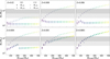 |
Fig. 1 Masses of the He (circles) and CO (diamonds) cores for the wind model from S23 (full markers) and C15 (void markers). The (light) gray shaded areas represent the regime for (pulsational) pair-instability supernovae. |
3 Results
3.1 Stellar cores
Figure 1 shows the final He and CO core masses for the S23 and C15 wind models. At low metallicity (Z ≤ 0.0001), the two wind models predict the same monotonic increase of the He and CO core mass with MZAMS, because VMSs do not enter the optically thick wind regime. At these metallicities, the C15 models generally yield slightly smaller cores, due to the different envelope undershooting and convection models (Simonato et al. 2025).
At higher metallicity, the two considered models C15 and S23 behave in a dramatically different way. According to S23, VMSs can enter the optically thick wind regime at Z ≥ 0.001: such strong winds reduce the final total mass and core mass of VMSs, resulting in a flat or even decreasing trend of Mc with MZAMS. Hence, the S23 model predicts smaller He and CO cores compared to C15, with a significant impact on the occurrence of (pulsational) pair instability.
The effect of optically thick winds in the S23 model is twofold. On the one hand, the S23 model results in a lower metallicity threshold below which VMSs can enter the (pulsational) pair instability regime: the threshold is Zth = 0.004 and 0.01 for S23 and C15, respectively. On the other hand, the formation of IMBHs via direct collapse is suppressed in the S23 model for metallicity Z ≥ 0.001, whereas the C15 model allows the formation of IMBHs at Z ≤ 0.008 because of the lower wind mass loss.
For example, at Z = 0.001 optically thick winds become effective for MZAMS > 200 M⊙, when the stellar core is already well within the pair-instability regime. Mass loss prevents the He core mass from increasing above 135 M⊙. As a consequence, only VMSs with MZAMS ≳ 450 M⊙ undergo direct collapse into a IMBH in the S23 model, whereas in C15 IMBHs can form via direct collapse at MZAMS ~ 300 M⊙.
For Z = 0.004, VMSs with MZAMS ≥ 200 M⊙ develop stellar winds that are strong enough to reduce the stellar core to Mc < 30 M⊙, where even pulsational pair instability is inhibited. For Z ≳ 0.006, VMSs in the S23 models undergo optically thick stellar winds throughout the mass range considered. This dramatically reduces the final core masses, which display a weak dependence on MZAMS. For example, at Z ~ 0.006 the core mass for VMSs with MZAMS > 400 M⊙ decreases from ~200 M⊙ in the C15 model to ~20 M⊙ in S23.
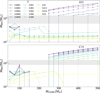 |
Fig. 2 Final BH mass as a function of MZAMS for different metallicities, Z, for the S23 (upper) and C15 (lower) wind mass-loss prescription. The gray shaded area shows the resulting pair-instability mass gap for the two wind models. |
3.2 BH masses
Figure 2 shows the final BH mass as a function of MZAMS for models C15 and S23. The key difference between the two models is the metallicity threshold to form IMBHs; this is ZIMBH = 0.001 and 0.012 for models S23 and C15, respectively. In model S23, IMBH formation is suppressed at metallicity Z > 0.001 by the onset of optically thick winds. These strong winds erode the mass of the He core and prevent it from reaching the threshold MHe ~ 135 M⊙, above which the star avoids exploding as a pair-instability supernova. Thus, even the most massive stars do not produce IMBHs in the S23 model unless they have metallicity Z ≤ 0.001. In contrast, the lower mass loss in model C15 allows larger cores to grow and enables the formation of IMBHs up to Z ~ 0.012.
In the absence of optically thick winds, the BH mass increases with MZAMS, up to the onset of (pulsational) pair instability, at MZAMS ≳ 75 M⊙. For larger initial masses, the onset of direct collapse depends on metallicity. In the C15 model, VMSs undergo (pulsational) pair instability up to Z = 0.01. At lower metallicities, all the models with MZAMS > 400 M⊙ produce IMBHs, with masses ranging from 135 M⊙ to 450 M⊙. At Z = 0.02, instead, wind mass loss is strong enough to prevent the onset of pair instability, leading to a maximum BH mass MBH ~ 30 M⊙.
In the S23 model, the maximum metallicity at which IMBHs form is an order of magnitude lower (Z = 0.001) compared to C15. Below this threshold, the S23 model produces IMBHs with masses in the same range as C15. At higher metallicities, the most massive BHs originate from stars with MZAMS ~ 50 M⊙, while more massive stars deliver MBH ≲ 15M⊙. This happens because VMSs develop optically thick winds at an early stage, and spend all their lifetime with ![Mathematical equation: $\[\dot{M}\]$](/articles/aa/full_html/2026/03/aa57817-25/aa57817-25-eq11.png) > 10−5 M⊙ yr−1. This results in a severe erosion of the core (Simonato et al. 2025; Boco et al. 2025). Overall, the S23 models predict a pair-instability BH mass gap from 65 M⊙ to 135 M⊙.
> 10−5 M⊙ yr−1. This results in a severe erosion of the core (Simonato et al. 2025; Boco et al. 2025). Overall, the S23 models predict a pair-instability BH mass gap from 65 M⊙ to 135 M⊙.
Figure 3 shows the final BH mass as a function of the ZAMS mass and the metallicity for the S23 model. The formation of IMBHs only takes place for VMSs with MZAMS ≳ 250 M⊙ at Z ≤ 0.001. Also, the formation of BHs with MBH > 20 M⊙ is suppressed for Z > 0.01 throughout the mass range.
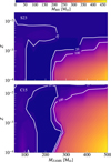 |
Fig. 3 Contour plot showing the final BH mass as a function of MZAMS and Z, for the S23 (upper panel) and the C15 (lower panel) models. The white contours highlight the levels at 20 M⊙ and 100 M⊙. |
3.3 BH mass function
3.3.1 BHs from single VMSs
Figure 4 shows the BH mass function from single VMSs assuming a Kroupa (Kroupa 2001) initial mass function. For Z > 0.001 optically thick winds strongly suppress the production of IMBHs from single stars. At Z = 0.001, the S23 model still allows IMBH formation, but the efficient mass loss limits the maximum BH mass to 150 M⊙, compared to 350 M⊙ in the C15 model. For higher metallicities, stellar winds progressively reduce the maximum BH mass in the S23 model, down to 20 M⊙ at Z = 0.02.
In the C15 model, the formation of IMBHs takes place up to Z = 0.01, where the maximum BH mass is ~180 M⊙ (also see Costa et al. 2025). At lower metallicities, the maximum IMBH mass reaches ~400 M⊙, for ZAMS masses up to MZams = 500 M⊙. In this model, IMBH formation from single VMSs is only suppressed at Z = 0.02, where BHs can form with a mass up to 33 M⊙.
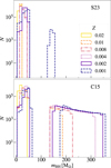 |
Fig. 4 Black hole mass distribution from single stars with MZAMS > 50 M⊙, for the models adopting the S23 (upper panel) and C15 (lower panel) wind prescriptions and for different metallicities. |
3.3.2 BBHs from VMS binaries
Figure 5 shows the primary BH masses from binaries with primary mass MZAMS,1 > 50M⊙, distributed according to a Kroupa (Kroupa 2001) mass function. We refer to Section 2.4 for more details on the initial conditions. We display the mass distribution of both primary BHs in BBHs and single BHs from disrupted binaries. Star-star collisions dramatically extend the BH mass function to larger values compared to the single stellar-evolution case in Fig. 4.
The C15 model predicts the formation of BHs as massive as ≳700 M⊙ for Z ≤ 0.002. Also, IMBHs up to ~400 M⊙ can still form at Z = 0.01. In the S23 model, instead, the formation of IMBHs is already suppressed at Z = 0.004, where they represent less than 0.2% of the total BH number, despite the occurrence of star-star colllisions. In contrast, the percentage of IMBHs is 21% in the C15 model at Z = 0.004. We find that, in the metallicity range Z = 0.004–0.008, our distributions are consistent with those from Shepherd et al. (2025) when they consider the same wind prescription.
Primary BHs in BBHs also reach higher masses than BHs from single stellar evolution, due to mass accretion from the stellar companion. In the S23 model, IMBH formation in BBHs is possible for Z ≤ 0.002, while for Z = 0.004, the maximum primary BH mass in BBHs decreases to 45 M⊙. At Z = 0.02, the BH mass function in the S23 model extends from 5 M⊙ to 20 M⊙.
Black holes in BBHs display a pair-instability mass gap between 65 M⊙ and 135 M⊙ for both the C15 and the S23 models. In contrast, star-star collisions can produce BHs in this mass range, and fill the pair-instability mass gap with single BHs.
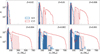 |
Fig. 5 Black hole mass distribution from binaries with MZAMS,1 > 50M⊙, for models adopting the S23 (solid blue line, solid fill) and C15 (dashed red line, hatched area) wind prescriptions. The shaded (hatched) areas indicate the BHs in BBHs, while the empty histograms display the single BHs from disrupted binaries, including BHs that form from stellar collisions. |
3.3.3 BBH mergers
Figures 6 and 7 show the primary and remnant mass distributions for BBHs that merge within a Hubble time. In the S23 model, no BBH merger has a primary mass m1 > 50 M⊙ for Z > 0.002. In the C15 case, IMBH mergers can occur up to a metallicity of Z = 0.004. In general, the BBH merger mass distribution displays a mild dependence on metallicity, with a peak at ~10 M⊙.
The maximum merger remnant produced by these BBHs is usually two times as massive as the maximum primary BH mass. In the presence of optically thick winds (model S23), the formation of IMBHs from BBH mergers is thus possible up to Z = 0.002, where mBH,max ~ 240 M⊙. At higher metallicities, the maximum BH remnant mass progressively decreases down to 35 M⊙ at Z = 0.02. In the C15 models, the masses delivered by BBH mergers are larger, with the possibility of having IMBH remnants up to a metallicity of Z = 0.006.
3.3.4 Progenitors of GW231123 and GW190521
We qualitatively compare our models with the most massive BBH mergers detected by the LIGO-Virgo-KAGRA interferometers, namely GW231123 (The LIGO Scientific Collaboration et al. 2025c) and GW190521 (Abbott et al. 2020b; Abbott et al. 2020a). According to our S23 model, the progenitors of GW231123 should have had a metallicity Z ≤ 0.002. The primary mass of GW190521 (Abbott et al. 2020b; Abbott et al. 2020a), instead, lies well within the mass gap predicted by both our C15 and S23 models. In a follow-up work, we will explore the dynamical formation of such mergers with our new S23 models (Torniamenti et al., in prep.).
4 Discussion
4.1 Impact of rotation and overshooting
In this work, we investigate the impact of a recent model that accounts for optically thick winds (S23) in the formation of IMBHs from VMSs. We considered nonrotating stellar models with a fixed overshooting parameter. However, both stellar rotation and core overshooting may have a relevant impact on the final BH mass. In a follow-up paper, we will include these additional parameters in detail. In the following, we briefly discuss their expected impact on our results.
Stellar rotation affects both the envelope and the core mass, leading to enhanced stellar-mass loss during the main sequence (Langer 1998, but also see Müller & Vink 2014), and triggering chemical mixing in the core (Sabhahit et al. 2023). In the optically thin regime, rotation generally results in enhanced mass loss when the critical rotation is approached (Ω/Ωc > 0.4). As a consequence, it can further quench the BH production at low metallicity Z < 0.01 Z⊙, where optically thick winds are not activated (Winch et al. 2024, 2025). Also, rotation can drive the transition to the optically thick regime at lower initial masses (Sabhahit et al. 2023; Boco et al. 2025). For VMSs, this mainly affects the evolution at low Z, where the star can retain a large fraction of its angular momentum due to weaker mass loss. At high Z, wind mass loss can efficiently remove the angular momentum, leading to a minor impact from stellar rotation on the final BH mass.
Core overshooting also triggers chemical mixing, affecting the final core mass in a similar way to rotation (Sabhahit et al. 2022). In the optically thin regime, increasing the overshooting parameter leads to more massive cores, with larger values of MBH for the same MZAMS (Winch et al. 2024). For VMSs, optically thick winds already lead to the formation of a fully mixed star if the initial stellar mass is large enough (MZAMS > 200 M⊙, Sabhahit et al. 2022), while removing the stellar envelope. As a consequence, overshooting is not expected to play an important role in the final BH mass.
In summary, we expect overshooting and rotation to affect the relation between MZAMS and MBH in the low-metallicity and low-mass end of the parameter space considered, where mass loss is driven by optically thin winds. In such regimes, a larger overshooting parameter and a fast rotation may further reduce the maximum value of Z at which IMBHs are produced. When more vigorous stellar winds are present, VMS evolution is expected to be mainly driven by stellar mass loss, with a less relevant impact from these parameters.
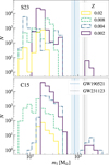 |
Fig. 6 Primary BH mass distribution in BBH mergers with MZAMS,1 > 50M⊙, for the S23 (upper) and C15 (lower) wind prescriptions, and for different metallicities. The dashed blue (dotted black) line displays the inferred value for GW190521 (GW231123), with the estimated uncertainty (shaded area). |
4.2 Caveats of VMS population models
In our population-synthesis models, we drew primary stellar masses from a Kroupa IMF between 50 and 500 M⊙, corresponding to the extreme high-mass end of the mass function. In most star-forming regions, the presence of stars in this mass range is dominated by stochastic effects or possibly by additional quenching effects (e.g., Weidner & Kroupa 2006). Thus, the conclusions of our population-synthesis simulations only apply to extreme star-forming regions, such as the R136 cluster in the LMC (Crowther et al. 2010; Bestenlehner et al. 2020), the super-star clusters in starburst galaxies (e.g., the Antennae galaxies, Whitmore & Schweizer 1995), and the high-redshift massive clusters recently discovered by the James Webb Space Telescope (Vanzella et al. 2023; Adamo et al. 2024; Mowla et al. 2024). Moreover, it is also possible that VMSs are the result of multiple stellar collisions in very dense star clusters (Portegies Zwart & McMillan 2002). In such case, population studies require dedicated N–body simulations (e.g., Di Carlo et al. 2021; Rantala et al. 2024).
5 Conclusions
We investigated the impact of a new optically thick wind model (S23) on the formation of IMBHs in nonrotating isolated single and binary very massive stars (VMSs). The new model is supported by several observational constraints, such as the pair-instability supernova rate (Simonato et al. 2025) and the existence of single Wolf–Rayet stars at low metallicity (Boco et al. 2025). We integrated the evolution of VMSs with MESA (Paxton et al. 2019) and folded our new MESA tracks inside our binary population-synthesis code SEVN (Iorio et al. 2023).
We find that IMBH production is suppressed at intermediate metallicity (Z ∈ [10−3, 0.01]), compared to less effective wind models. According to our models, IMBHs cannot form from VMS collapse at the metallicity of the LMC (Z ~ 0.008) and possibly even the Small Magellanic Cloud (Z ~ 0.0025).
Intermediate mass black holes might be able to form via stellar collisions at a metallicity as high as Z = 0.004, but only under the very optimistic assumption that each collision triggers no mass loss. However, even with this assumption for stellar collisions, the occurrence fraction of IMBHs over the total number of BHs (≲0.2%) is two orders of magnitude lower compared to models with less effective wind mass loss.
Binary BH mergers can produce IMBH remnants at metallicity Z ≤ 0.002. At higher metallicities, the enhanced mass loss produces BBH mergers with primary mass m1 < 50 M⊙, making it impossible to form IMBHs from first-generation BH mergers.
The BH mass spectrum from single VMSs shows a pair-instability mass gap from 65 M⊙ to 135 M⊙. Such a mass gap is still present in the mass distribution of BHs in BBHs and BBH mergers.
According to our S23 models, the progenitors of the most massive BBH observed by the LIGO-Virgo-KAGRA collaboration, GW231123 (The LIGO Scientific Collaboration et al. 2025c), must have had a metallicity Z ≤ 0.002. In a follow-up study, we will explore the impact of star cluster dynamics on this result.
Acknowledgements
We thank the anonymous referee for their insightful comments and suggestions. We thank Gautham Sabhahit and collaborators for sharing their MESA inlists (https://github.com/Apophis-1/VMS_Paper1, https://github.com/Apophis-1/VMS_Paper2). We thank Guglielmo Costa and Kendall Shepherd for useful comments and discussions. ST acknowledges financial support from the Alexander von Humboldt Foundation for the Humboldt Research Fellowship. ST, MM and GI acknowledge financial support from the European Research Council for the ERC Consolidator grant DEMOBLACK, under contract no. 770017. ST, MM and LB also acknowledge financial support from the German Excellence Strategy via the Heidelberg Cluster of Excellence (EXC 2181 – 390900948) STRUCTURES. GI acknowledges financial support from the La Caixa Foundation for the La Caixa Junior Leader fellowship 2024. GI also acknowledges financial support under the National Recovery and Resilience Plan (NRRP), Mission 4, Component 2, Investment 1.4, – Call for tender No. 3138 of 18/12/2021 of Italian Ministry of University and Research funded by the European Union – NextGenerationEU. EK and MM acknowledge support from the PRIN grant METE under contract No. 2020KB33TP. EK acknowledges financial support from the Fondazioni Gini for the Gini grant. The authors acknowledge support by the state of Baden-Württemberg through bwHPC and the German Research Foundation (DFG) through grants INST 35/1597-1 FUGG and INST 35/1503-1 FUGG. We use the MESA software (https://docs.mesastar.org/en/latest/) version r12115; (Paxton et al. 2011, 2013, 2015, 2018, 2019). We use SEVN (https://gitlab.com/sevncodes/sevn) to generate our BBHs catalogs (Spera et al. 2019; Mapelli et al. 2020; Iorio et al. 2023), TRACKCRUNCHER (https://gitlab.com/sevncodes/trackcruncher) (Iorio et al. 2023) to produce the tables for the interpolation. The PARSEC stellar tracks that we used for this work are publicly available at http://stev.oapd.inaf.it/PARSEC/ (Costa et al. 2025). This research made use of NUMPY (Harris et al. 2020), PANDAS (The pandas development Team 2024), SCIPY (Virtanen et al. 2020) and MATPLOTLIB (Hunter 2007).
References
- Abbott, R., Abbott, T. D., Abraham, S., et al. 2020a, ApJ, 900, L13 [NASA ADS] [CrossRef] [Google Scholar]
- Abbott, R., Abbott, T. D., Abraham, S., et al. 2020b, Phys. Rev. Lett., 125, 101102 [Google Scholar]
- Adamo, A., Bradley, L. D., Vanzella, E., et al. 2024, Nature, 632, 513 [NASA ADS] [CrossRef] [Google Scholar]
- Antonini, F., Gieles, M., & Gualandris, A. 2019, MNRAS, 486, 5008 [NASA ADS] [CrossRef] [Google Scholar]
- Antonini, F., Gieles, M., Dosopoulou, F., & Chattopadhyay, D. 2023, MNRAS, 522, 466 [NASA ADS] [CrossRef] [Google Scholar]
- Antonini, F., Romero-Shaw, I., Callister, T., et al. 2025, arXiv e-prints [arXiv:2509.04637] [Google Scholar]
- Arca Sedda, M., Kamlah, A. W. H., Spurzem, R., et al. 2023, MNRAS, 526, 429 [NASA ADS] [CrossRef] [Google Scholar]
- Ballone, A., Costa, G., Mapelli, M., et al. 2023, MNRAS, 519, 5191 [NASA ADS] [CrossRef] [Google Scholar]
- Baumgardt, H., He, C., Sweet, S. M., et al. 2019, MNRAS, 488, 5340 [CrossRef] [Google Scholar]
- Belczynski, K., Bulik, T., Fryer, C. L., et al. 2010, ApJ, 714, 1217 [NASA ADS] [CrossRef] [Google Scholar]
- Belkus, H., Van Bever, J., & Vanbeveren, D. 2007, ApJ, 659, 1576 [NASA ADS] [CrossRef] [Google Scholar]
- Bestenlehner, J. M., Crowther, P. A., Caballero-Nieves, S. M., et al. 2020, MNRAS, 499, 1918 [Google Scholar]
- Bestenlehner, J. M., Gräfener, G., Vink, J. S., et al. 2014, A&A, 570, A38 [NASA ADS] [CrossRef] [EDP Sciences] [Google Scholar]
- Boco, L., Mapelli, M., Sander, A. A. C., et al. 2025, A&A, 703, A243 [NASA ADS] [CrossRef] [EDP Sciences] [Google Scholar]
- Bressan, A., Marigo, P., Girardi, L., et al. 2012, MNRAS, 427, 127 [NASA ADS] [CrossRef] [Google Scholar]
- Burrows, A., & Vartanyan, D. 2021, Nature, 589, 29 [CrossRef] [PubMed] [Google Scholar]
- Burrows, A., Wang, T., & Vartanyan, D. 2024, ApJ, 964, L16 [NASA ADS] [CrossRef] [Google Scholar]
- Chen, Y., Bressan, A., Girardi, L., et al. 2015, MNRAS, 452, 1068 [Google Scholar]
- Choi, J., Dotter, A., Conroy, C., et al. 2016, ApJ, 823, 102 [Google Scholar]
- Costa, G., Girardi, L., Bressan, A., et al. 2019a, A&A, 631, A128 [NASA ADS] [CrossRef] [EDP Sciences] [Google Scholar]
- Costa, G., Girardi, L., Bressan, A., et al. 2019b, MNRAS, 485, 4641 [NASA ADS] [CrossRef] [Google Scholar]
- Costa, G., Bressan, A., Mapelli, M., et al. 2021, MNRAS, 501, 4514 [NASA ADS] [CrossRef] [Google Scholar]
- Costa, G., Ballone, A., Mapelli, M., & Bressan, A. 2022, MNRAS, 516, 1072 [NASA ADS] [CrossRef] [Google Scholar]
- Costa, G., Shepherd, K. G., Bressan, A., et al. 2025, A&A, 694, A193 [NASA ADS] [CrossRef] [EDP Sciences] [Google Scholar]
- Cox, J. P., & Giuli, R. T. 1968, Principles of Stellar Structure [Google Scholar]
- Crowther, P. A., Schnurr, O., Hirschi, R., et al. 2010, MNRAS, 408, 731 [Google Scholar]
- de Jager, C., Nieuwenhuijden, H., & van der Hucht, K. A. 1988, Bull. Inform. Centre Donnees Stellaires, 35, 141 [Google Scholar]
- Di Carlo, U. N., Mapelli, M., Pasquato, M., et al. 2021, MNRAS, 507, 5132 [NASA ADS] [CrossRef] [Google Scholar]
- Dotter, A. 2016, ApJS, 222, 8 [Google Scholar]
- Farmer, R., Renzo, M., de Mink, S. E., Marchant, P., & Justham, S. 2019, ApJ, 887, 53 [Google Scholar]
- Farmer, R., Renzo, M., de Mink, S. E., Fishbach, M., & Justham, S. 2020, ApJ, 902, L36 [CrossRef] [Google Scholar]
- Fernández, R., Quataert, E., Kashiyama, K., & Coughlin, E. R. 2018, MNRAS, 476, 2366 [CrossRef] [Google Scholar]
- Fishbach, M., Holz, D. E., & Farr, B. 2017, ApJ, 840, L24 [NASA ADS] [CrossRef] [Google Scholar]
- Freitag, M., Gürkan, M. A., & Rasio, F. A. 2006a, MNRAS, 368, 141 [NASA ADS] [Google Scholar]
- Freitag, M., Rasio, F. A., & Baumgardt, H. 2006b, MNRAS, 368, 121 [NASA ADS] [CrossRef] [Google Scholar]
- Fryer, C. L., Belczynski, K., Wiktorowicz, G., et al. 2012, ApJ, 749, 91 [Google Scholar]
- Gerosa, D., & Berti, E. 2017, Phys. Rev. D, 95, 124046 [NASA ADS] [CrossRef] [Google Scholar]
- Gerosa, D., & Fishbach, M. 2021, Nat. Astron., 5, 749 [NASA ADS] [CrossRef] [Google Scholar]
- Gräfener, G., & Hamann, W. R. 2008, A&A, 482, 945 [Google Scholar]
- Greene, J. E., Strader, J., & Ho, L. C. 2020, ARA&A, 58, 257 [Google Scholar]
- Grevesse, N., & Sauval, A. J. 1998, Space Sci. Rev., 85, 161 [Google Scholar]
- Häberle, M., Neumayer, N., Seth, A., et al. 2024, Nature, 631, 285 [CrossRef] [Google Scholar]
- Harris, C. R., Millman, K. J., van der Walt, S. J., et al. 2020, Nature, 585, 357 [NASA ADS] [CrossRef] [Google Scholar]
- Heger, A., & Woosley, S. E. 2002, ApJ, 567, 532 [Google Scholar]
- Herwig, F. 2000, A&A, 360, 952 [NASA ADS] [Google Scholar]
- Hunter, J. D. 2007, Comput. Sci. Eng., 9, 90 [NASA ADS] [CrossRef] [Google Scholar]
- Iorio, G., Mapelli, M., Costa, G., et al. 2023, MNRAS, 524, 426 [NASA ADS] [CrossRef] [Google Scholar]
- Jermyn, A. S., Bauer, E. B., Schwab, J., et al. 2023, ApJS, 265, 15 [NASA ADS] [CrossRef] [Google Scholar]
- Kıroğlu, F., Kremer, K., Biscoveanu, S., González Prieto, E., & Rasio, F. A. 2025a, ApJ, 979, 237 [Google Scholar]
- Kıroğlu, F., Kremer, K., & Rasio, F. A. 2025b, ApJ, 994, L37 [Google Scholar]
- Kroupa, P. 2001, MNRAS, 322, 231 [NASA ADS] [CrossRef] [Google Scholar]
- Langer, N. 1998, A&A, 329, 551 [NASA ADS] [Google Scholar]
- Ledoux, P. 1947, ApJ, 105, 305 [NASA ADS] [CrossRef] [Google Scholar]
- Lovegrove, E., & Woosley, S. E. 2013, ApJ, 769, 109 [NASA ADS] [CrossRef] [Google Scholar]
- Magg, E., Bergemann, M., Serenelli, A., et al. 2022, A&A, 661, A140 [NASA ADS] [CrossRef] [EDP Sciences] [Google Scholar]
- Mapelli, M. 2016, MNRAS, 459, 3432 [NASA ADS] [CrossRef] [Google Scholar]
- Mapelli, M., Zampieri, L., Ripamonti, E., & Bressan, A. 2013, MNRAS, 429, 2298 [NASA ADS] [CrossRef] [Google Scholar]
- Mapelli, M., Spera, M., Montanari, E., et al. 2020, ApJ, 888, 76 [NASA ADS] [CrossRef] [Google Scholar]
- Mapelli, M., Dall’Amico, M., Bouffanais, Y., et al. 2021, MNRAS, 505, 339 [CrossRef] [Google Scholar]
- Marchant, P., Renzo, M., Farmer, R., et al. 2019, ApJ, 882, 36 [Google Scholar]
- Martins, F., Hillier, D. J., Paumard, T., et al. 2008, A&A, 478, 219 [NASA ADS] [CrossRef] [EDP Sciences] [Google Scholar]
- Mezcua, M. 2017, Int. J. Mod. Phys. D, 26, 1730021 [Google Scholar]
- Miller-Jones, J. C. A., Wrobel, J. M., Sivakoff, G. R., et al. 2012, ApJ, 755, L1 [Google Scholar]
- Moe, M., & Di Stefano, R. 2017, ApJS, 230, 15 [Google Scholar]
- Mowla, L., Iyer, K., Asada, Y., et al. 2024, Nature, 636, 332 [Google Scholar]
- Müller, P. E., & Vink, J. S. 2014, A&A, 564, A57 [CrossRef] [EDP Sciences] [Google Scholar]
- Nguyen, C. T., Costa, G., Girardi, L., et al. 2022, A&A, 665, A126 [NASA ADS] [CrossRef] [EDP Sciences] [Google Scholar]
- O’Connor, E., & Ott, C. D. 2011, ApJ, 730, 70 [Google Scholar]
- Paxton, B., Bildsten, L., Dotter, A., et al. 2011, ApJS, 192, 3 [Google Scholar]
- Paxton, B., Cantiello, M., Arras, P., et al. 2013, ApJS, 208, 4 [Google Scholar]
- Paxton, B., Marchant, P., Schwab, J., et al. 2015, ApJS, 220, 15 [Google Scholar]
- Paxton, B., Schwab, J., Bauer, E. B., et al. 2018, ApJS, 234, 34 [NASA ADS] [CrossRef] [Google Scholar]
- Paxton, B., Smolec, R., Schwab, J., et al. 2019, ApJS, 243, 10 [Google Scholar]
- Pols, O. R., Schröder, K.-P., Hurley, J. R., Tout, C. A., & Eggleton, P. P. 1998, MNRAS, 298, 525 [Google Scholar]
- Portegies Zwart, S. F., Makino, J., McMillan, S. L. W., & Hut, P. 1999, A&A, 348, 117 [NASA ADS] [Google Scholar]
- Portegies Zwart, S. F., & McMillan, S. L. W. 2002, ApJ, 576, 899 [Google Scholar]
- Rantala, A., Naab, T., & Lahén, N. 2024, MNRAS, 531, 3770 [NASA ADS] [CrossRef] [Google Scholar]
- Renzo, M., Farmer, R. J., Justham, S., et al. 2020, MNRAS, 493, 4333 [NASA ADS] [CrossRef] [Google Scholar]
- Rizzuto, F. P., Naab, T., Spurzem, R., et al. 2021, MNRAS, 501, 5257 [NASA ADS] [CrossRef] [Google Scholar]
- Romagnolo, A., Gormaz-Matamala, A. C., & Belczynski, K. 2024, ApJ, 964, L23 [NASA ADS] [CrossRef] [Google Scholar]
- Sabhahit, G. N., Vink, J. S., Higgins, E. R., & Sander, A. A. C. 2022, MNRAS, 514, 3736 [NASA ADS] [CrossRef] [Google Scholar]
- Sabhahit, G. N., Vink, J. S., Sander, A. A. C., & Higgins, E. R. 2023, MNRAS, 524, 1529 [NASA ADS] [CrossRef] [Google Scholar]
- Sana, H., de Mink, S. E., de Koter, A., et al. 2012, Science, 337, 444 [Google Scholar]
- Sander, A. A. C., & Vink, J. S. 2020, MNRAS, 499, 873 [Google Scholar]
- Sander, A. A. C., Hamann, W. R., Todt, H., et al. 2019, A&A, 621, A92 [NASA ADS] [CrossRef] [EDP Sciences] [Google Scholar]
- Shepherd, K. G., Costa, G., Ugolini, C., et al. 2025, A&A, 701, A126 [NASA ADS] [CrossRef] [EDP Sciences] [Google Scholar]
- Simonato, F., Torniamenti, S., Mapelli, M., et al. 2025, A&A, 703, A215 [NASA ADS] [CrossRef] [EDP Sciences] [Google Scholar]
- Spera, M., & Mapelli, M. 2017, MNRAS, 470, 4739 [Google Scholar]
- Spera, M., Mapelli, M., Giacobbo, N., et al. 2019, MNRAS, 485, 889 [Google Scholar]
- Stothers, R. B. 1999, MNRAS, 305, 365 [NASA ADS] [CrossRef] [Google Scholar]
- The LIGO Scientific Collaboration, the Virgo Collaboration, & the KAGRA Collaboration 2025a, arXiv e-prints [arXiv:2508.18083] [Google Scholar]
- The LIGO Scientific Collaboration, The Virgo Collaboration, & the KAGRA Collaboration 2025b, arXiv e-prints [arXiv:2508.18082] [Google Scholar]
- The LIGO Scientific Collaboration, the Virgo Collaboration, the KAGRA Collaboration, et al. 2025, arXiv e-prints [arXiv:2507.08219] [Google Scholar]
- The pandas development Team 2024, pandas-dev/pandas: Pandas [Google Scholar]
- Torniamenti, S., Rastello, S., Mapelli, M., et al. 2022, MNRAS, 517, 2953 [NASA ADS] [CrossRef] [Google Scholar]
- Torniamenti, S., Mapelli, M., Périgois, C., et al. 2024, A&A, 688, A148 [NASA ADS] [CrossRef] [EDP Sciences] [Google Scholar]
- Tremou, E., Strader, J., Chomiuk, L., et al. 2018, ApJ, 862, 16 [Google Scholar]
- Vanbeveren, D., Belkus, H., Van Bever, J., & Mennekens, N. 2009, Ap&SS, 324, 271 [Google Scholar]
- Vanzella, E., Claeyssens, A., Welch, B., et al. 2023, ApJ, 945, 53 [NASA ADS] [CrossRef] [Google Scholar]
- Vink, J. S. 2018, A&A, 615, A119 [NASA ADS] [CrossRef] [EDP Sciences] [Google Scholar]
- Vink, J. S., & Gräfener, G. 2012, ApJ, 751, L34 [Google Scholar]
- Vink, J. S., de Koter, A., & Lamers, H. J. G. L. M. 2000, A&A, 362, 295 [Google Scholar]
- Vink, J. S., de Koter, A., & Lamers, H. J. G. L. M. 2001, A&A, 369, 574 [NASA ADS] [CrossRef] [EDP Sciences] [Google Scholar]
- Vink, J. S., Muijres, L. E., Anthonisse, B., et al. 2011, A&A, 531, A132 [NASA ADS] [CrossRef] [EDP Sciences] [Google Scholar]
- Vink, J. S., Heger, A., Krumholz, M. R., et al. 2015, Highlights Astron., 16, 51 [Google Scholar]
- Virtanen, P., Gommers, R., Oliphant, T. E., et al. 2020, Nat. Methods, 17, 261 [Google Scholar]
- Weidner, C., & Kroupa, P. 2006, MNRAS, 365, 1333 [Google Scholar]
- Whitmore, B. C., & Schweizer, F. 1995, AJ, 109, 960 [NASA ADS] [CrossRef] [Google Scholar]
- Winch, E. R. J., Vink, J. S., Higgins, E. R., & Sabhahitf, G. N. 2024, MNRAS, 529, 2980 [NASA ADS] [CrossRef] [Google Scholar]
- Winch, E. R. J., Sabhahit, G. N., Vink, J. S., & Higgins, E. R. 2025, MNRAS, 540, 90 [Google Scholar]
- Woosley, S. E. 2017, ApJ, 836, 244 [Google Scholar]
- Woosley, S. E., Blinnikov, S., & Heger, A. 2007, Nature, 450, 390 [NASA ADS] [CrossRef] [PubMed] [Google Scholar]
- Yungelson, L. R., van den Heuvel, E. P. J., Vink, J. S., Portegies Zwart, S. F., & de Koter, A. 2008, A&A, 477, 223 [NASA ADS] [CrossRef] [EDP Sciences] [Google Scholar]
The MESA inlists and run_star_extras files by Sabhahit et al. (2023) are publicly available at this link.
Here, we refer to the traditionally considered value for solar metallicity Z = 0.02 (Grevesse & Sauval 1998; but see, e.g., Magg et al. 2022 for more recent estimates).
The PARSEC stellar tracks are publicly available at http://stev.oapd.inaf.it/PARSEC/ (Costa et al. 2025).
All Figures
|
Fig. 1 Masses of the He (circles) and CO (diamonds) cores for the wind model from S23 (full markers) and C15 (void markers). The (light) gray shaded areas represent the regime for (pulsational) pair-instability supernovae. |
| In the text | |
|
Fig. 2 Final BH mass as a function of MZAMS for different metallicities, Z, for the S23 (upper) and C15 (lower) wind mass-loss prescription. The gray shaded area shows the resulting pair-instability mass gap for the two wind models. |
| In the text | |
|
Fig. 3 Contour plot showing the final BH mass as a function of MZAMS and Z, for the S23 (upper panel) and the C15 (lower panel) models. The white contours highlight the levels at 20 M⊙ and 100 M⊙. |
| In the text | |
|
Fig. 4 Black hole mass distribution from single stars with MZAMS > 50 M⊙, for the models adopting the S23 (upper panel) and C15 (lower panel) wind prescriptions and for different metallicities. |
| In the text | |
|
Fig. 5 Black hole mass distribution from binaries with MZAMS,1 > 50M⊙, for models adopting the S23 (solid blue line, solid fill) and C15 (dashed red line, hatched area) wind prescriptions. The shaded (hatched) areas indicate the BHs in BBHs, while the empty histograms display the single BHs from disrupted binaries, including BHs that form from stellar collisions. |
| In the text | |
|
Fig. 6 Primary BH mass distribution in BBH mergers with MZAMS,1 > 50M⊙, for the S23 (upper) and C15 (lower) wind prescriptions, and for different metallicities. The dashed blue (dotted black) line displays the inferred value for GW190521 (GW231123), with the estimated uncertainty (shaded area). |
| In the text | |
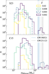 |
Fig. 7 Same as Fig. 6, but for the resulting BH remnant mass. |
| In the text | |
Current usage metrics show cumulative count of Article Views (full-text article views including HTML views, PDF and ePub downloads, according to the available data) and Abstracts Views on Vision4Press platform.
Data correspond to usage on the plateform after 2015. The current usage metrics is available 48-96 hours after online publication and is updated daily on week days.
Initial download of the metrics may take a while.