| Issue |
A&A
Volume 707, March 2026
|
|
|---|---|---|
| Article Number | A312 | |
| Number of page(s) | 9 | |
| Section | Stellar structure and evolution | |
| DOI | https://doi.org/10.1051/0004-6361/202557835 | |
| Published online | 16 March 2026 | |
Fates of the sub-stellar objects (FOSSO)
I. Fates of the known brown dwarfs in main-sequence–BD binaries
1
School of Physics and Astronomy, Sun Yat-sen University, Zhuhai 519082, PR China
2
CSST Science Center for the Guangdong-HongKong-Macau Great Bay Area, Sun Yat-sen University, Zhuhai 519082, PR China
3
Yunnan Observatories, Chinese Academy of Sciences, Kunming 650216, PR China
4
International Centre of Supernovae, Yunnan Key Laboratory, Kunming 650216, PR China
5
University of Chinese Academy of Sciences, Beijing 100049, PR China
★ Corresponding authors: This email address is being protected from spambots. You need JavaScript enabled to view it.
, This email address is being protected from spambots. You need JavaScript enabled to view it.
Received:
26
October
2025
Accepted:
16
January
2026
Abstract
Context. Understanding the survival and orbital evolution of brown dwarf (BD) companions during the post-main-sequence (MS) evolution of their host stars has become increasingly important, especially following recent discoveries of substellar companions around white dwarfs (WDs).
Aims. We investigated the long-term evolution and final outcomes of BDs orbiting low-mass MS stars as these evolve into WDs. By comparing forward-modelled populations with observed WD–BD binaries, we tested evolutionary models and predicted the existence of yet-undetected systems.
Methods. We employed the code Compact Object Mergers: Population Astrophysics and Statistics (COMPAS) to evolve observed MS–BD systems through the post-MS phases of their host stars into the WD stage, tracking orbital changes driven by mass loss, tides, and common-envelope (CE) evolution.
Results. Our simulations reproduce a period gap in the distribution of detached WD–BD binaries, consistent with observations. We also identify a boundary separating detached and semi-detached systems in the period-mass diagram at orbital periods of ∼1−2 hours, depending on the BD mass.
Conclusions. We predict that a subset of currently known MS–BD binaries will survive post-MS evolution and emerge as detached WD–BD systems, while others will undergo CE evolution and potentially form cataclysmic variables with BD donors. Our results reproduce the observed period gap in WD–BD binaries and provide quantitative predictions for the role of CE efficiency in shaping their distribution. These findings indicate that many WD–BD systems remain undetected, motivating targeted searches using microlensing and high-contrast imaging techniques with next-generation large telescopes.
Key words: binaries: close / brown dwarfs / white dwarfs
© The Authors 2026
 Open Access article, published by EDP Sciences, under the terms of the Creative Commons Attribution License (https://creativecommons.org/licenses/by/4.0), which permits unrestricted use, distribution, and reproduction in any medium, provided the original work is properly cited.
This article is published in open access under the Subscribe to Open model. This email address is being protected from spambots. You need JavaScript enabled to view it. to support open access publication.
1. Introduction
Brown dwarfs (BDs) are substellar objects that occupy the mass regime between giant planets and low-mass stars, typically defined as having masses between 13 and 75 Jupiter masses (MJup; Burrows et al. 2001). Unlike stars, BDs lack sufficient mass to sustain stable hydrogen fusion in their cores and therefore never reach the main sequence. The detection of thousands of BDs, including a significant fraction in binary systems (Feng et al. 2022), has provided invaluable data that inform both the planetary and stellar formation processes. A notable feature in the population statistics of BDs orbiting FGK-type main-sequence (MS) stars is the ‘brown dwarf desert’ (BDD), characterised by a paucity of intermediate-mass BDs in close orbits (Halbwachs et al. 2000; Marcy & Butler 2000; Troup et al. 2016; Shahaf & Mazeh 2019). This deficit suggests distinct formation mechanisms for BDs of different masses (Grether & Lineweaver 2006; Ma & Ge 2014), a hypothesis further supported by analyses of orbital and stellar property distributions. For example, using a sample compiled from observation of radial velocity (RV), transit, and astrometry, Ma & Ge (2014) proposed a transition mass around 42.5 MJup that separates the eccentricity distributions of lower- and higher-mass BD. More recently, Giacalone et al. (2026) compiled a long-period BD sample from RV observation of the California Legacy Survey and found a metallicity transition mass around 27 MJup that separates metal-rich hosts of lower-mass companions from metal-poor hosts of higher-mass companions. However, some studies of short-period transiting BD samples do not support such a transition between planetary and stellar formation (e.g. Vowell et al. 2025), suggesting that additional observations are needed to confirm this picture.
The long-term dynamical evolution of substellar companions, particularly BDs and planets, around FGK-type stars is a critical area of astrophysical research. These host stars eventually evolve off the MS, passing through giant phases before becoming white dwarfs (WDs). During this post-MS evolution, physical processes such as stellar mass loss, tidal interactions, and stellar wind accretion can profoundly alter the orbital parameters and even the masses of their companions (Nordhaus et al. 2010; Veras et al. 2011). Although the survivability and dynamical fates of planetary companions have been extensively studied (Villaver & Livio 2009; Veras et al. 2011; Nordhaus & Spiegel 2013; Mustill et al. 2014), investigations specifically dedicated to BDs in this context remain comparatively less explored.
Owing to their significantly larger masses compared to giant planets, BDs are more likely to survive the common-envelope (CE) phase, thereby facilitating the formation of close WD–BD binary systems (Nordhaus & Spiegel 2013). Their greater mass also leads to stronger tidal interactions with their evolving host stars. Studies of BD evolution during the post-MS stage are therefore crucial for constraining poorly understood binary interaction parameters, such as those governing the CE phase, and for testing theories related to the BDD (Zorotovic & Schreiber 2022; Chen et al. 2024). Despite the identification of more than a thousand BD candidates orbiting MS stars (Gaia Collaboration 2023; Kiefer et al. 2025), only a limited number of BDs orbiting WDs have been confirmed (e.g. Casewell et al. 2018b). This observational scarcity is primarily due to the intrinsic faintness of BDs, which makes their detection challenging in WD systems. Nevertheless, population synthesis models predict a substantial, yet largely unobserved, population of WD–BD binaries that evolved from MS–BD progenitors over gigayear timescales (Zorotovic & Schreiber 2022; Chen et al. 2024).
This paper, the first of the Fates of the Sub-stellar Objects (hereafter FOSSO I), addresses this gap by investigating the long-term evolution of a comprehensive sample of observed BD companions to A-, F-, G-, and K-type stars. We used detailed numerical simulations to trace their evolution through the post-main-sequence phases of their host stars into the WD stage. Our primary objectives are: (1) to predict the ultimate fates and orbital distributions of these BDs; (2) to compare our simulated WD–BD populations with the currently observed sample in order to validate and refine formation and evolutionary models; and (3) to provide guidance for future observational campaigns aimed at discovering new WD–BD systems. By focusing on the distinct post-MS evolutionary behaviour of BDs, this study seeks to bridge the gap between planetary and stellar companion evolution, thereby contributing to a more complete picture of substellar populations and their role in binary stellar evolution.
The structure of this paper is as follows: Section 2 describes the observational datasets of MS–BD and WD–BD binary systems used in our analysis. Section 3 presents the numerical methods and the simulation results. We provide a comprehensive discussion of our findings in Section 4, followed by our conclusions in Section 5.
2. Data and observation
We compiled a dataset of 196 known MS–BD binaries from the literature to investigate the future fate and distribution of these systems. In Section 3, we show that most of these systems are expected to evolve into either close or wide WD–BD binaries. Additionally, we collected data on 22 known WD–BD binaries to compare them with the predicted evolution of known MS–BD binaries.
2.1. The BD companion of an MS star
We primarily compiled the observational data for the MS–BD binaries analysed in this study from recent literature Rosenthal et al. (2021), Grieves et al. (2021), Feng et al. (2022), Stevenson et al. (2023), Rothermich et al. (2024), Kiefer et al. (2025), Vowell et al. (2025), publicly accessible astronomical databases (Schneider et al. 2011; Han et al. 2014), and references therein. We cross-checked the data between catalogues and applied the following selection criteria:
-
(1)
The BD has a measured mass within the range 13−75 MJup;
-
(2)
The host star has a mass between 0.9−8.0 M⊙, ensuring it can evolve into a WD within 13.7 billion years;
-
(3)
The metallicity, Z, of the host star lies between 0.001−0.03;
-
(4)
The host star is in its MS evolutionary stage;
-
(5)
The orbital period of the system is less than 108 days.
These criteria yield 196 MS–BD binary systems. The complete catalogue, which includes system parameters and corresponding references, is publicly available (see Data availability system). Figure 1 shows the BD mass-orbital period distribution of this sample, with colour encoding the MS mass. The top and right panels present histograms of the orbital period and BD mass, respectively. We also calculated and plotted the kernel density estimates (KDEs) of the distributions. Most of the MS stars in the sample are solar-type, with masses near 1 M⊙. Their expected WD remnants cover two mass ranges: systems experiencing CE evolution produce lower-mass WDs (0.4–0.5 M⊙; e.g. Zorotovic & Schreiber 2022), while those avoiding CE evolution follow single-star evolution and produce typical-mass WDs (0.5–0.6 M⊙; Hurley et al. 2000, 2002). The BD companions exhibit a relatively uniform mass distribution, with a shallow gap around the 42.5 MJup transition mass proposed by Ma & Ge (2014). Orbital periods are mainly concentrated between 103 and 104 days, with a gap around 105 days likely due to observational biases between methods.
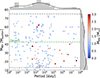 |
Fig. 1. Mass–period distribution of observed MS–BD binary systems used in this study. The colour scale indicates the mass of the host MS star. The top and right histograms, with kernel density estimates (KDEs), show the distributions of the orbital period and BD mass, respectively. The dashed grey lines indicate the BD mass range, while the dashed green line marks the BD desert transition mass of 42.5 MJup from Ma & Ge (2014). |
2.2. The BD companion around WDs
To date, only 11 detached close (Porb < 12 hour) WD–BD binary systems have been identified: SDSS J1411+2009 (WD+T5; Beuermann et al. 2013; Littlefair et al. 2014); SDSS J1205−0242 (WD+L0; Parsons et al. 2017; Rappaport et al. 2017); WD 1032+011 (WD+L5; Casewell et al. 2020); ZTF J0038+2030 (WD+BD; van Roestel et al. 2021); WD 0137−349 (WD+L8; Maxted et al. 2006; Burleigh et al. 2006); NLTT 5306 (WD+dL5; Steele et al. 2013); SDSS J1557+0916 (WD+L3–L5; Farihi et al. 2017); EPIC 212235321 (WD+L3; Casewell et al. 2018b); GD 1400 (WD+L6–L7; Farihi & Christopher 2004; Dobbie et al. 2005; Burleigh et al. 2011; Casewell et al. 2024); WD 0837+185 (WD+T8; Casewell et al. 2012); and SDSS J1231+0041 (WD+M/L; Parsons et al. 2017). In addition, 11 wide (Porb > 100 yr) WD–BD binary systems have been identified: KMT-2020-BLG-0414 (Zhang et al. 2024a); PHL 5038 (WD+L8; Steele et al. 2009); GD 165 (WD+L4; Becklin & Zuckerman 1988); SDSS J2225+0016 (WD+L4; French et al. 2023); LSPM J0055+5948 (WD+T8; Meisner et al. 2020); COCONUTS-1 (WD+T4; Zhang et al. 2020); VVV J1256−6202 (WD+L3; Zhang et al. 2024b); Wolf 1130 C (Mace et al. 2013, 2018; Burgasser et al. 2025); WD 0806−661 (WD+Y1; Luhman et al. 2011); LSPM J1459+0851 (WD+T4.5; Day-Jones et al. 2011); and LSPM J0241+2553 (Deacon et al. 2014). Among these systems, nine close systems and ten wide systems possess reliable and precise measurement data. The system parameters of these 19 systems are summarised in Table 1.
Parameters of WD–BD binaries from observations.
Recent Hubble Space Telescope (HST) studies of BD atmospheres continue to refine our understanding of cloud structure, spectral behaviour, and atmospheric dynamics across the L-T-Y sequence. Time-resolved near-infrared spectroscopy with the HST wide field camera 3 (WFC3) has shown that the variability in L- and T-transition objects is primarily driven by heterogeneous cloud thickness and large-scale atmospheric circulation rather than simple clearing (Apai et al. 2013; Buenzli et al. 2014). The HST imaging programmes targeting T8–Y1 dwarfs provide important constraints on binarity and system architecture (Fontanive et al. 2023). For WD–BD systems such as GD 1400, HST observations also provide complementary constraints on BD atmospheres, revealing cloud coverage, day-night temperature contrasts, and efficient heat redistribution (Amaro et al. 2025). These studies highlight the role of HST in probing the physical and dynamical characteristics of BDs.
As shown in Table 2, throughout this paper we focus on four sample sets. All but 19 observed WD–BD binaries come from simulations based on the observed MS–BD binaries using the binary evolutionary models discussed in Section 3.1. Here and throughout the paper, the terms ‘simulation’ or ‘simulated system’ refer to these samples.
WD–BD binary samples.
3. Methods and results
3.1. Evolution of the MS–BD binary
We used the code Compact Object Mergers: Population Astrophysics and Statistics (COMPAS; Riley et al. 2022) to simulate their evolution of the observed MS–BD binary systems during the primary star’s post-MS stage over the age of the Universe. The COMPAS code is designed for fast population synthesis of binary evolution and is based on the single-star evolution (SSE; Hurley et al. 2000) and binary star evolution (BSE; Hurley et al. 2002) models. We modified the code to calculate the evolution of MS–BD binaries (Chen et al. 2024).
In the post-MS stage of the primary, the orbital evolution of a binary system constitutes a variable-mass two-body problem (Veras 2016). During this stage, two factors significantly affect the companion’s orbital evolution: mass loss (ML) and tidal interactions between the two stars in the binary (Nordhaus & Spiegel 2013). The primary’s mass loss is mostly attributed to the rapid stellar wind loss process. In this case, the timescale of primary mass loss is much longer than the orbital period, a scenario known as the Jeans mode (Huang 1963). Considering the conservation of angular momentum in the system, the evolution of the orbital semi-major axis a is given by
 (1)
(1)
where Mtot = MMS + MBD is the total mass of the binary. When the primary evolves off the MS and reaches the giant branch stage, it undergoes significant radius expansion and mass loss. As a result, its companion moves to a wider orbit, while the eccentricity remains unchanged. Moreover, stellar tidal interactions transfer orbital angular momentum to the star’s spin angular momentum, leading to orbital decay, circularisation, and spin-up of the primary star. In our simulation, we considered orbital evolution under both equilibrium and dynamical tides, derived by Kapil et al. (in preparation), based on Zahn (1977), which is included in the latest version of COMPAS (Team Compas 2025).
For close MS–BD binaries (P ≲ 1000 d), orbital expansion driven by mass loss may not be sufficient to prevent engulfment by the expanding primary star. If the primary’s envelope fills its Roche lobe (RL), mass transfer can occur via RL overflow (RLOF). Following Eggleton (1983), the equivalent RL radius can be estimated as
 (2)
(2)
where q = MMS/MBD is the mass ratio of the primary star to the companion. According to Ge et al. (2020, 2023, 2024), mass transfer in binaries with an initial mass ratio larger than a critical value tends to be unstable. Once mass transfer becomes unstable, the primary’s core and the companion BD are soon surrounded by the primary’s envelope, which is known as the common envelope (CE) phase. During this phase, the stellar core and the BD spiral inwards due to dynamical interaction with the envelope material (Livio & Soker 1988), eventually leading to orbital decay and circularisation. If the binary has sufficient energy to disperse the CE, it becomes an extremely close post-CE binary. Following Xu & Li (2010), the orbital decay can be expressed as
 (3)
(3)
where M1, c and M1, e are the core and envelope masses of the primary star, respectively. The parameter λ represents the envelope binding energy factor, for which we adopted the prescription of Xu & Li (2010). The coefficient αCE denotes the energy transform rate, which is estimated to be ∼0.3 for MS–BD binaries (Zorotovic & Schreiber 2022; Chen et al. 2024). After the CE is dispersed, MS–BD binaries ultimately evolve into WD–BD binaries with close and circular orbits.
Using a population synthesis method, Chen et al. (2024) identify and characterise two evolutionary channels linking close MS–BD binaries to post-CE WD–BD binaries, resulting in two corresponding classes, as shown in their Figure 1 and Section 3. The main difference between the two channels is the evolutionary stage at which the system enters the CE phase:
-
Channel A: CE occurs during the primary’s red giant branch stage, and the system is likely to form a helium-core WD–BD binary.
-
Channel B: CE occurs during the primary’s asymptotic giant branch stage, and the system is likely to form a carbon-oxygen-core WD–BD binary.
For example, recent research (e.g. Zhang et al. 2024a) suggests that relatively wide post-CE WD–BD binaries may form following channel B in Chen et al. (2024). In these close WD–BD binaries, the orbits continue to shrink due to angular-momentum loss (AML) from gravitational wave (GW) radiation. We computed the orbital decay due to GW radiation from the moment after CE dispersal to the age of the Universe using the expression from Schreiber & Gänsicke (2003):
 (4)
(4)
where tcooling is the WD cooling time.
As suggested by Schreiber & Gänsicke (2003), a post-CE binary system containing a WD and an MS or M-dwarf companion can evolve into a cataclysmic variable (CV) due to GW-induced AML and companion expansion, eventually initiating mass transfer through RLOF. In this traditional evolutionary channel, the donor is initially stellar and evolves towards shorter orbital periods until reaching the period minimum, after which further mass loss produces a partially degenerate donor and a period-bounce phase (e.g. Rappaport et al. 1982; Knigge et al. 2011; McAllister et al. 2017). Consequently, many CVs hosting BD-mass donors likely reached the substellar boundary through stable mass loss rather than originating from WD–BD binaries (e.g. McAllister et al. 2017). In contrast, post-CE WD–BD binaries can form CVs through a different evolutionary pathway. Unlike MS or M-dwarf stars, the structure of BDs can be well described by the polytropic model with index n = 1.5. Their interiors, supported by electron degeneracy pressure, can be regarded as uniform-density convective cores (Burrows et al. 2001). When a BD approaches its host WD, tidal forces can cause its radius to expand and fill its RL. In this case, material from the BD transfers to the WD via RLOF, potentially forming an accretion disc around the WD and eventually transforming the system into a CV (e.g. Casewell et al. 2018a,b; Rappaport et al. 2017). Because the BD is partially degenerate, the post-CE WD–BD binary can initiate RLOF at orbital periods shorter than typical WD–MS or M-dwarf binaries. For example, Rappaport et al. (2017) show that the very short-period transiting BD in the pre-CV binary WD 1202−024 (SDSS J1205−0242) will evolve into a CV system in the near future. Close post-CE WD–BD systems have a minimum allowed orbital period, below which the BD fills its RL and initiates mass transfer. In our simulation, we calculate the minimum period of post-CE WD–BD binaries following Equation (16) of Rappaport et al. (2021):
 (5)
(5)
where Pmin, BD is expressed in minutes. In our simulation, some systems, despite having enough energy to disperse the CE, end up with orbital periods below Pmin, BD. This outcome suggests that the BDs in these systems are tidally disrupted during the CE phase, eventually merging with the primary and producing single WDs.
For wide MS–BD binaries (P ≳ 1000 d), except for extremely eccentric systems (e ≳ 0.9), the tidal dissipation in the primary stars has little effect on their orbits due to the large separation. Consequently, the BD companion in such systems does not experience a CE phase. Instead, the primary’s mass loss drives the BD to a wider orbit as the primary star evolves into a WD. Similarly, Jovian planets on wide orbits can avoid engulfment and survive the post-MS evolution of their host stars. Such objects around nearby WDs may be detectable via infrared imaging (Burleigh et al. 2002).
3.2. Evolution results
Adopting the evolutionary framework described in Section 3.1, we calculated the evolutionary fate of 196 MS–BD binaries selected in Section 2.1. Figures 2 and 3 show the results of these simulations. In our simulation, 94 binaries do not experience a CE phase and remain wide WD–BD binaries, while 102 binaries undergo a CE phase during the GB stage of the primary star. Of the 102 systems experiencing the CE phase, 91 merge during CE and evolve into single WDs, while the remaining 11 systems survive as detached WD–BD binaries after CE dispersal: BD+63 974 b, HD 156312 Bb, HD 115517 b, HD 30246 b, HD 87646 Ac, HD 104289 b, HD 140913 b, HD 132032 b, HD 5433 b, HD 136118 b, and KOI-415 b. Table 3 lists the orbital parameters of these post-CE systems, including the final stellar mass, orbital period, and the timescales for the primary to evolve into a WD and subsequently reach the CV phase. We calculated these quantities using Equations (4) and (5).
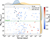 |
Fig. 2. Same as Fig. 1, all symbols represent the initial MS–BD systems, while different shapes indicate the different fates. The top and right KDE plots show the distributions of different outcomes: grey, blue, and orange correspond to merged systems, close WD–BD systems, and wide WD–BD systems, respectively. |
Parameters of WD–BD binaries surviving the CE in our simulations (αCE = 0.3).
Figure 2 shows the distribution of the initial parameters, with different symbols indicating their different fates of the sample systems. From the top and right KDE curves, systems with a more massive BD and an intermediate initial orbital period (100−1000 days) are more likely to form post-CE WD–BD binaries. Figure 3 shows the period-mass distribution of future WD–BD binary systems. The upper and lower panels correspond to results with and without tidal dissipation effects, respectively. As noted by Nordhaus & Spiegel (2013), the combined effects of mass-loss-induced orbital expansion, tidal dissipation, and CE-ejection-induced orbital decay create a period gap in the distribution of substellar companions around their host WDs. For the future WD–BD population, we identify a period gap of approximately 1 to 1000 days. Confirmed WD–BD binaries listed in Table 1 are marked with star symbols and lie on either side of the period gap, in good agreement with our simulation results. The dashed grey line indicates the minimum allowed orbital period, below which systems are likely to become CVs. To date, no detached or semi-detached CV systems containing low-mass BDs with periods below this minimum have been observed, suggesting that the majority of these systems merged during the CE phase.
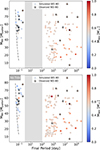 |
Fig. 3. Period-mass distribution of predicted WD–BD systems formed from the observed MS–BD binaries, calculated with tidal effects (top panel) and without tidal effects (bottom panel). Stars mark the observed close and wide WD–BD binaries listed in Table 1. The grey area indicates the period gap between about 1 and 1000 days. The dashed line indicates the minimum period for the binaries to evolve into CVs. |
Figure 4 shows changes in the semi-major axis of MS–BD binaries that successfully evolve into WD–BD binaries. Close systems that undergo CE evolution experience significant orbital decay, whereas wider systems that avoid CE experience orbital expansion. Consequently, a separation gap appears at the WD–BD stage, approximately between 1 and 1000 R⊙. We also plot the minimum orbital separation for a rough comparison, derived from the average Roche lobe radius of the BDs in the surviving systems. Systems with separations smaller than this limit are likely to become semi-detached and enter the CV phase. Other close systems gradually approach this limit through GW radiation emission, eventually evolving into CVs.
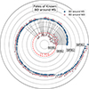 |
Fig. 4. Fates of known BDs around MS stars. Blue and pink dots represent the initial and final separations of surviving MS–BD binaries. The dot size indicates the mass of the BDs. The dashed red circle shows the average minimum separations required for binaries to remain detached. |
3.3. Mass-ratio and period distribution of WD–BD systems
We performed a comparative analysis between the post-CE close and no-CE wide WD–BD binaries from simulation and observation. Figure 5 shows the cumulative distribution functions (CDFs) of the mass ratio q = MBD/MWD for the simulated and observed WD–BD binaries. Solid and dashed lines represent close and wide systems, respectively. The simulation results indicate that the close systems have notably higher mass ratios than the wide systems. This trend can be explained by CE evolutionary models: the CE-dispersal process can cut off the growth of the primary’s core, leading to a less massive WD. Meanwhile, heavier BDs are more likely to survive the CE phase, resulting in higher mass ratios for close systems. As shown in the left panel, the close binary systems in the observational sample exhibit relatively high mass ratios, consistent with the simulation results. However, the current sample remains small, and future observations are required to confirm this feature.
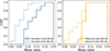 |
Fig. 5. Cumulative distribution functions (CDFs) of the mass ratio q = MBD/MWD. Left panel: Mass ratio distribution of close and wide simulated samples. Right panel: Distribution of the observed samples. |
To further test the binary evolutionary models, we compared the orbital period distributions between the simulated and observed WD–BD binaries. Figure 6 presents cumulative distribution functions (CDFs) of orbital periods for close and wide systems. For close systems, the CDFs of the simulations and observations are in good agreement, with a Kolmogorov-Smirnov test p-value of 0.59, indicating that the adopted CE model and the αCE value are appropriate. For wide systems, the simulated and observed samples show a discrepancy in their period CDFs. Because wide binaries are difficult to detect, this difference is likely due to observational biases from different detection methods, as further discussed in Section 4.5.
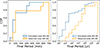 |
Fig. 6. Cumulative distribution functions (CDFs) of orbital periods for WD–BD binaries. Left panel: Comparison of orbital period distributions for close WD–BD systems from the simulated and observed samples. Right panel: Same comparison for the wide WD–BD systems. |
4. Discussion
In this section, we discuss the implications of our population synthesis results for the formation and observability of WD–BD binaries. Our models predict that the orbital period distribution is primarily shaped by whether systems undergo CE evolution, producing distinct post-CE and non-CE populations. This naturally generates a deficit of systems at intermediate periods, whose interpretation requires careful consideration given current observational limitations. We therefore assess the robustness of the predicted period structure, examine the main sources of model uncertainty, and compare our results with previous theoretical and observational studies. We conclude by discussing how future observations can test these predictions and refine our understanding of the formation and evolution of WD–substellar binaries.
4.1. Period gap
Our comprehensive investigation into the post-MS evolution of observed MS–BD binaries provides crucial insights into the formation and ultimate fates of substellar companions around WDs. Based on an MS–BD binaries catalogue and a theoretical evolutionary model, we predict the future period-mass distribution of WD–BD binaries and identify a period gap (see also Nordhaus & Spiegel 2013), broadly consistent with current observations.
However, the apparent ‘period gap’ around 1−1000 days in the distribution of WD–BD binaries should be interpreted with appropriate caution. In our evolutionary framework, a deficit of systems with orbital periods of ∼1−1000 days arises naturally from binary evolution physics: systems that undergo CE evolution are driven to very short periods, whereas systems that avoid CE evolution experience orbital expansion due to post-MS mass loss, resulting in much wider separations. Consequently, WD–BD binaries with intermediate periods are intrinsically rare in the simulations. The currently known WD–BD systems are broadly consistent with this theoretical expectation, with observed objects located on either side of the predicted gap. However, the total number of confirmed WD–BD binaries remains small, and observational selection effects cannot be excluded. Radial velocity and transit surveys preferentially detect short-period systems, whereas direct imaging and astrometric methods are most sensitive to wide companions, potentially producing an apparent deficit at intermediate periods.
A noteworthy exception is the transiting planetary-mass companion WD 1856+534 b (Vanderburg et al. 2020; Lagos et al. 2021). With an orbital period of ∼1.4 days, it lies near the boundary of the predicted gap. We emphasise, however, that WD 1856+534 b has a mass well below the BD regime and is therefore not directly comparable to the WD–BD population considered here. Owing to its lower mass, the minimum survivable post-CE orbital period for such a planet is longer than for typical BDs. Moreover, its formation may involve more complex evolutionary pathways, such as dynamically assisted or multi-body CE evolution (e.g. Chamandy et al. 2021). Thus, WD 1856+534 b does not contradict the predicted WD–BD period gap, but rather highlights the diversity of evolutionary outcomes for substellar companions. Overall, although current observations do not contradict the existence of a WD–BD period gap, larger and more complete samples are required to determine whether it represents an intrinsic outcome of binary evolution or is instead shaped primarily by observational biases.
4.2. Model uncertainties
Although our current model provides a robust framework for predicting the evolution of MS–BD binaries, we note areas where further refinement could improve the fidelity of our predictions. A primary assumption in our treatment of orbital evolution during stellar mass loss is the adiabatic Jeans mode approximation (Huang 1963). This approximation, valid when the mass-loss timescale significantly exceeds the orbital period, maintains constant eccentricity and precludes companion ejection. Although appropriate for close binaries, this assumption may break down for BDs on wide orbits around evolving stars, particularly if the orbits are highly eccentric. In such cases, the stellar mass-loss timescale can become comparable to the orbital period, leading to non-adiabatic effects that may excite orbital eccentricity or even eject the companion, producing free-floating BDs. Future work will explore the parameter space where non-adiabatic effects become dominant, potentially requiring more sophisticated N-body simulations coupled with stellar evolution models to accurately capture these complex dynamical outcomes.
Furthermore, the presence of tertiary or higher-order companions in some MS–BD systems introduces additional dynamical complexity. For simplicity, we assume that distant tertiary companions have a negligible gravitational influence on the evolution of the primary MS–BD binary. However, multi-body interactions can induce Kozai-Lidov cycles, secular perturbations, or scattering events that dramatically alter the BD’s orbit, particularly during phases of significant stellar mass loss. Incorporating a comprehensive N-body treatment alongside stellar evolution within a larger population synthesis framework represents a critical next step to accurately model these intricate systems and assess the impact of higher-order multiplicity on the ultimate fate of BD companions.
4.3. Comparison with previous studies
Our findings build upon and complement previous efforts to characterise WD–BD binary systems and their progenitors. Earlier studies by Zorotovic & Schreiber (2022) and Chen et al. (2024) used observed WD–BD data to constrain CE parameters and to test hypotheses related to the brown dwarf desert by retro-calculating progenitor systems. In contrast, our approach forward-evolves observed MS–BD systems, providing a predictive framework that allows direct comparison with existing and future WD–BD observations, thereby validating evolutionary models and anticipating undiscovered populations.
A significant improvement in our study is the explicit inclusion of tidal effects throughout the primary’s post-MS evolution. As shown in Figure 3, tidal dissipation can induce significant orbital decay and circularisation prior to the CE phase, influencing whether a system enters CE and its subsequent outcome. Our results indicate that tidal effects increase the number of systems entering the CE phase by approximately 10% compared to models neglecting tides. The strength of tidal interactions is highly sensitive to binary separation, scaling inversely with the seventh to eighth power, so their influence is negligible for extremely wide binaries but crucial for closer systems. Given the ongoing debate surrounding tidal models in binary evolution, the increasing number of observed close WD–BD binaries will provide invaluable empirical constraints, enabling refinement of these critical parameters in future simulations.
Brown dwarfs (BDs) represent a critical intermediate-mass regime, exhibiting evolutionary pathways distinct from lower-mass giant planets. Giant planets are less likely to survive the CE phase due to their lower masses (Nordhaus & Spiegel 2013), leading to the observed scarcity of close WD-planet systems (Vanderburg et al. 2020; Blackman et al. 2021), whereas brown dwarfs possess enhanced survival capabilities. The period gap that we identify in the WD–BD population, spanning approximately 1−1000 days, aligns well with theoretical predictions for substellar companions. Its inner edge is consistent with the findings for giant planets presented by Nordhaus & Spiegel (2013). This result demonstrates the unified physics that governs post-CE binary evolution across a range of companion masses.
4.4. The impact of CE efficiency αCE
The CE efficiency parameter, αCE, remains a cornerstone for modelling the outcomes of binary evolution involving CE phases. This parameter, which quantifies the efficiency of orbital energy conversion into envelope ejection, critically determines the fate of systems that enter CE. Previous studies, often focused on post-CE binaries containing WDs, suggest a relatively low αCE in the range 0.2−0.4 (Zorotovic et al. 2010; Toonen & Nelemans 2013; Camacho et al. 2014; Parsons et al. 2015; Hernandez et al. 2021; Zorotovic & Schreiber 2022; Scherbak & Fuller 2023; Chen et al. 2024). Recently, Ge et al. (2022) provided a more self-consistent method to calculate the binding energy that addresses both the remnant core response and the companion mass effect. Ge et al. (2024) also found an average CE efficiency parameter of 0.32. However, it need not be constant and may vary as a function of the initial mass ratio, depending on the progenitor mass and evolutionary stage.
Our simulations, which span αCE from 0.1 to 1.0 (Figure 7), illustrate its profound impact. As expected, higher αCE values, indicating more efficient energy transfer, lead to a higher proportion of systems successfully ejecting the CE and surviving as detached close WD–BD binaries. Conversely, lower αCE values result in more systems merging within the envelope or forming extremely close systems that rapidly evolve into CVs. The interplay between tidal dissipation and αCE is also evident: tidal effects bring systems closer, increasing the number of binaries entering the CE phase, and thus amplifying the importance of αCE in determining the ultimate distribution of WD–BD systems. Our results highlight the continued need to empirically constrain αCE through precise observations of post-CE binaries.
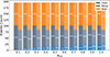 |
Fig. 7. Distribution of MS–BD binary systems with different evolutionary outcomes as a function of the CE efficiency parameter αCE. The bars show the counts of three different evolutionary outcomes: wide WD–BD binaries (orange), merged systems (grey), and detached close WD–BD binaries (blue). For each fixed αCE value, the darker bars indicate results with tidal effects, and lighter bars show those without. |
4.5. Implication for future observations
Our study provides guidance for future observational campaigns targeting substellar companions to WDs.
One prediction from our simulations is the existence of a population of WD–BD binaries with orbital periods of approximately 100 years, corresponding to separations of approximately 15 AU. This population remains largely undetected, likely due to observational biases: direct imaging techniques favour very wide separations, while radial velocity and photometric (eclipsing or transiting) methods are most sensitive to short-period systems. However, next-generation high-contrast imaging facilities and precision astrometry missions may be ideally positioned to uncover these systems and to measure their orbital properties. Recently, imaging observations of nearby metal-polluted WDs with the Mid-Infrared Instrument (MIRI) on the James Webb Space Telescope (JWST) have revealed candidate planetary-mass companions, including Jovian planets and low-mass BDs (Mullally et al. 2024, 2025; Debes et al. 2025; Albert et al. 2025). For example, the MIRI Excesses around Degenerates (MEAD) survey with the JWST reports a directly imaged candidate BD companion to a WD, MEAD 62 B (Albert et al. 2025). If confirmed, this BD candidate, with a mass of ∼14 MJup and a projected separation of ∼40 AU, would represent a valuable wide WD–BD system. Furthermore, microlensing surveys, which have already detected BDs around MS stars at these intermediate separations, hold significant promise. The recent discovery of a BD in the KMT-2020-BLG-0104 multi-body system around a WD via microlensing (Zhang et al. 2024a) validates this approach, suggesting that systematic microlensing campaigns could bridge this observational gap.
Moreover, our simulations predict that approximately 20 systems will evolve into semi-detached WD–BD binaries, destined to become cataclysmic variables with BD donors (BD-CVs). Although some such systems have been identified (Hernández Santisteban et al. 2016; Harrison 2016; Pala et al. 2019; Neustroev & Mäntynen 2023), their rarity underscores the need for targeted observational efforts. These systems serve as laboratories for studying mass transfer from substellar objects to WDs, the evolution of accretion discs, and the physics of highly irradiated BDs. Continued spectroscopic and photometric monitoring with facilities such as the HST and the Very Large Telescope (VLT), coupled with efforts to identify new BD-CV candidates from wide-field surveys, will provide invaluable data to test our evolutionary models and refine our understanding of the physical properties of giant planets and brown dwarfs under extreme conditions.
5. Conclusions
In this study, Project FOSSO I, we investigated the long-term orbital evolution of a sample of approximately 200 observed BDs orbiting solar-type MS stars. Using numerical simulations with the COMPAS code, we traced the evolution of these systems as their host stars transitioned through post-MS phases and ultimately became WDs. Our primary goal was to predict the fates and orbital characteristics of the resulting WD–BD binaries and to compare these predictions with current observational data.
Our simulations reveal that the initial properties of MS–BD binaries fundamentally dictate their post-MS evolution. We find that these systems generally evolve into either very close or wide WD–BD binaries, forming a period gap of 1−1000 days in the distribution of WD–BD binaries. This predicted gap agrees with the period distribution of currently observed WD–BD systems, providing strong validation for our evolutionary models.
For close MS–BD systems, the CE phase plays a critical role. Depending on the efficiency of energy transfer (αCE), a significant fraction of these systems either merge during the CE phase or emerge as extremely close post-CE binaries. Following Rappaport et al. (2021), we identify a minimum orbital period boundary for detached WD–BD systems, estimated to lie between 40 and 120 minutes and decreasing with increasing BD mass. Systems with periods below this threshold are predicted to evolve into semi-detached systems, potentially forming CVs with BD donors. Our analysis suggests that approximately 20 systems from our initial sample are likely to evolve into such CVs.
Conversely, wide MS–BD systems avoid the CE phase and experience orbital expansion due to stellar mass loss during their host stars’ giant phases. Our models predict a substantial population of WD–BD binaries with orbital periods of about 100 years (separations of ∼15 AU) that remain largely undiscovered. The current lack of observed systems in this regime likely results from observational biases, as direct imaging typically targets much wider separations, whereas radial velocity and eclipsing methods favour much shorter periods. Future advancements in high-contrast imaging, astrometry surveys, and microlensing observations hold great promise for detecting these predicted wide WD–BD systems, potentially expanding the known population. The recent microlensing detection of a BD companion in the KMT-2020-BLG-0104 multi-body system around a WD (Zhang et al. 2024a) exemplifies the potential of this method.
This study enhances our understanding of the long-term evolution of substellar companions and provides valuable insights for constraining binary evolution parameters, particularly those governing CE physics and tidal interactions. Continued observations of both detached WD–BD binaries and CVs with BD donors will be crucial for further refining these models and elucidating the full spectrum of fates for brown dwarfs in binary systems, thereby advancing the study of substellar objects and binary stellar evolution.
Data availability
The complete catalogue of MS–BD systems is available at the CDS via https://cdsarc.cds.unistra.fr/viz-bin/cat/J/A+A/707/A312
Acknowledgments
We acknowledge the financial support from the National Key R&D Program of China (2020YFC2201400), NSFC grant 12403071, 12073092, 12103097, 12103098, the science research grants from the China Manned Space Project (No. CMS-CSST-2021-B09). HG acknowledges the support from the Strategic Priority Research Program of the Chinese Academy of Sciences (grant No. XDB1160201), the National Natural Science Foundation of China (NSFC Nos. 12288102, 12525304), the National Key R&D Program of China (No. 2021YFA1600403).
References
- Albert, L., Poulsen, S. R., Le Bourdais, É., et al. 2025, ArXiv e-prints [arXiv:2510.12601] [Google Scholar]
- Amaro, R. C., Apai, D., Zhou, Y., et al. 2025, ApJ, 979, 231 [Google Scholar]
- Apai, D., Radigan, J., Buenzli, E., et al. 2013, ApJ, 768, 121 [NASA ADS] [CrossRef] [Google Scholar]
- Becklin, E. E., & Zuckerman, B. 1988, Nature, 336, 656 [Google Scholar]
- Beuermann, K., Dreizler, S., Hessman, F. V., et al. 2013, A&A, 558, A96 [NASA ADS] [CrossRef] [EDP Sciences] [Google Scholar]
- Blackman, J. W., Beaulieu, J. P., Bennett, D. P., et al. 2021, Nature, 598, 272 [NASA ADS] [CrossRef] [Google Scholar]
- Buenzli, E., Apai, D., Radigan, J., Reid, I. N., & Flateau, D. 2014, ApJ, 782, 77 [NASA ADS] [CrossRef] [Google Scholar]
- Burgasser, A. J., Gonzales, E. C., Beiler, S. A., et al. 2025, Science, 390, 697 [Google Scholar]
- Burleigh, M. R., Clarke, F. J., & Hodgkin, S. T. 2002, MNRAS, 331, L41 [Google Scholar]
- Burleigh, M. R., Hogan, E., Dobbie, P. D., Napiwotzki, R., & Maxted, P. F. L. 2006, MNRAS, 373, L55 [Google Scholar]
- Burleigh, M. R., Steele, P. R., Dobbie, P. D., et al. 2011, AIP Conf. Ser., 1331, 262 [Google Scholar]
- Burrows, A., Hubbard, W. B., Lunine, J. I., & Liebert, J. 2001, Rev. Mod. Phys., 73, 719 [Google Scholar]
- Camacho, J., Torres, S., García-Berro, E., et al. 2014, A&A, 566, A86 [NASA ADS] [CrossRef] [EDP Sciences] [Google Scholar]
- Casewell, S. L., Burleigh, M. R., Wynn, G. A., et al. 2012, ApJ, 759, L34 [NASA ADS] [CrossRef] [Google Scholar]
- Casewell, S. L., Littlefair, S. P., Parsons, S. G., et al. 2018a, MNRAS, 481, 5216 [NASA ADS] [CrossRef] [Google Scholar]
- Casewell, S. L., Braker, I. P., Parsons, S. G., et al. 2018b, MNRAS, 476, 1405 [NASA ADS] [CrossRef] [Google Scholar]
- Casewell, S. L., Belardi, C., Parsons, S. G., et al. 2020, MNRAS, 497, 3571 [NASA ADS] [CrossRef] [Google Scholar]
- Casewell, S. L., Burleigh, M. R., Napiwotzki, R., et al. 2024, MNRAS, 535, 753 [Google Scholar]
- Chamandy, L., Blackman, E. G., Nordhaus, J., & Wilson, E. 2021, MNRAS, 502, L110 [NASA ADS] [CrossRef] [Google Scholar]
- Chen, Z., Chen, Y., Chen, C., Ge, H., & Ma, B. 2024, A&A, 687, A256 [NASA ADS] [CrossRef] [EDP Sciences] [Google Scholar]
- Day-Jones, A. C., Pinfield, D. J., Ruiz, M. T., et al. 2011, MNRAS, 410, 705 [NASA ADS] [CrossRef] [Google Scholar]
- Deacon, N. R., Liu, M. C., Magnier, E. A., et al. 2014, ApJ, 792, 119 [NASA ADS] [CrossRef] [Google Scholar]
- Debes, J. H., Poulsen, S., Messier, A., et al. 2025, AJ, 170, 123 [Google Scholar]
- Dobbie, P. D., Burleigh, M. R., Levan, A. J., et al. 2005, MNRAS, 357, 1049 [Google Scholar]
- Eggleton, P. P. 1983, ApJ, 268, 368 [Google Scholar]
- Farihi, J., & Christopher, M. 2004, AJ, 128, 1868 [Google Scholar]
- Farihi, J., Parsons, S. G., & Gänsicke, B. T. 2017, Nat. Astron., 1, 0032 [NASA ADS] [CrossRef] [Google Scholar]
- Feng, F., Butler, R. P., Vogt, S. S., et al. 2022, ApJS, 262, 21 [NASA ADS] [CrossRef] [Google Scholar]
- Fontanive, C., Bedin, L. R., De Furio, M., et al. 2023, MNRAS, 526, 1783 [NASA ADS] [CrossRef] [Google Scholar]
- French, J. R., Casewell, S. L., Dupuy, T. J., et al. 2023, MNRAS, 519, 5008 [CrossRef] [Google Scholar]
- Gaia Collaboration (Arenou, F., et al.) 2023, A&A, 674, A34 [CrossRef] [EDP Sciences] [Google Scholar]
- Ge, H., Webbink, R. F., & Han, Z. 2020, ApJS, 249, 9 [NASA ADS] [CrossRef] [Google Scholar]
- Ge, H., Tout, C. A., Chen, X., et al. 2022, ApJ, 933, 137 [NASA ADS] [CrossRef] [Google Scholar]
- Ge, H., Tout, C. A., Chen, X., et al. 2023, ApJ, 945, 7 [NASA ADS] [CrossRef] [Google Scholar]
- Ge, H., Tout, C. A., Webbink, R. F., et al. 2024, ApJ, 961, 202 [NASA ADS] [CrossRef] [Google Scholar]
- Giacalone, S., Howard, A. W., Gilbert, G. J., et al. 2026, AJ, 171, 75 [Google Scholar]
- Grether, D., & Lineweaver, C. H. 2006, ApJ, 640, 1051 [Google Scholar]
- Grieves, N., Bouchy, F., Lendl, M., et al. 2021, A&A, 652, A127 [NASA ADS] [CrossRef] [EDP Sciences] [Google Scholar]
- Halbwachs, J. L., Arenou, F., Mayor, M., Udry, S., & Queloz, D. 2000, A&A, 355, 581 [Google Scholar]
- Han, E., Wang, S. X., Wright, J. T., et al. 2014, PASP, 126, 827 [NASA ADS] [CrossRef] [Google Scholar]
- Harrison, T. E. 2016, ApJ, 816, 4 [NASA ADS] [CrossRef] [Google Scholar]
- Hernández Santisteban, J. V., Knigge, C., Littlefair, S. P., et al. 2016, Nature, 533, 366 [Google Scholar]
- Hernandez, M. S., Schreiber, M. R., Parsons, S. G., et al. 2021, MNRAS, 501, 1677 [Google Scholar]
- Huang, S.-S. 1963, ApJ, 138, 471 [NASA ADS] [CrossRef] [Google Scholar]
- Hurley, J. R., Pols, O. R., & Tout, C. A. 2000, MNRAS, 315, 543 [Google Scholar]
- Hurley, J. R., Tout, C. A., & Pols, O. R. 2002, MNRAS, 329, 897 [Google Scholar]
- Kiefer, F., Lagrange, A.-M., Rubini, P., & Philipot, F. 2025, A&A, 702, A77 [NASA ADS] [CrossRef] [EDP Sciences] [Google Scholar]
- Knigge, C., Baraffe, I., & Patterson, J. 2011, ApJS, 194, 28 [Google Scholar]
- Lagos, F., Schreiber, M. R., Zorotovic, M., et al. 2021, MNRAS, 501, 676 [Google Scholar]
- Littlefair, S. P., Casewell, S. L., Parsons, S. G., et al. 2014, MNRAS, 445, 2106 [NASA ADS] [CrossRef] [Google Scholar]
- Livio, M., & Soker, N. 1988, ApJ, 329, 764 [Google Scholar]
- Luhman, K. L., Burgasser, A. J., & Bochanski, J. J. 2011, ApJ, 730, L9 [NASA ADS] [CrossRef] [Google Scholar]
- Ma, B., & Ge, J. 2014, MNRAS, 439, 2781 [Google Scholar]
- Mace, G. N., Kirkpatrick, J. D., Cushing, M. C., et al. 2013, ApJ, 777, 36 [Google Scholar]
- Mace, G. N., Mann, A. W., Skiff, B. A., et al. 2018, ApJ, 854, 145 [NASA ADS] [CrossRef] [Google Scholar]
- Marcy, G. W., & Butler, R. P. 2000, PASP, 112, 137 [Google Scholar]
- Maxted, P. F. L., Napiwotzki, R., Dobbie, P. D., & Burleigh, M. R. 2006, Nature, 442, 543 [NASA ADS] [CrossRef] [Google Scholar]
- McAllister, M. J., Littlefair, S. P., Dhillon, V. S., et al. 2017, MNRAS, 467, 1024 [NASA ADS] [CrossRef] [Google Scholar]
- Meisner, A. M., Faherty, J. K., Kirkpatrick, J. D., et al. 2020, ApJ, 899, 123 [NASA ADS] [CrossRef] [Google Scholar]
- Mullally, S. E., Debes, J., Cracraft, M., et al. 2024, ApJ, 962, L32 [NASA ADS] [CrossRef] [Google Scholar]
- Mullally, F., Mullally, S. E., Cracraft, M., et al. 2025, ArXiv e-prints [arXiv:2512.08191] [Google Scholar]
- Mustill, A. J., Veras, D., & Villaver, E. 2014, MNRAS, 437, 1404 [CrossRef] [Google Scholar]
- Neustroev, V. V., & Mäntynen, I. 2023, MNRAS, 523, 6114 [NASA ADS] [CrossRef] [Google Scholar]
- Nordhaus, J., & Spiegel, D. S. 2013, MNRAS, 432, 500 [NASA ADS] [CrossRef] [Google Scholar]
- Nordhaus, J., Spiegel, D. S., Ibgui, L., Goodman, J., & Burrows, A. 2010, MNRAS, 408, 631 [NASA ADS] [CrossRef] [Google Scholar]
- Pala, A. F., Gänsicke, B. T., Marsh, T. R., et al. 2019, MNRAS, 483, 1080 [NASA ADS] [CrossRef] [Google Scholar]
- Parsons, S. G., Agurto-Gangas, C., Gänsicke, B. T., et al. 2015, MNRAS, 449, 2194 [NASA ADS] [CrossRef] [Google Scholar]
- Parsons, S. G., Hermes, J. J., Marsh, T. R., et al. 2017, MNRAS, 471, 976 [NASA ADS] [CrossRef] [Google Scholar]
- Rappaport, S., Joss, P. C., & Webbink, R. F. 1982, ApJ, 254, 616 [NASA ADS] [CrossRef] [Google Scholar]
- Rappaport, S., Vanderburg, A., Nelson, L., et al. 2017, MNRAS, 471, 948 [Google Scholar]
- Rappaport, S., Vanderburg, A., Schwab, J., & Nelson, L. 2021, ApJ, 913, 118 [Google Scholar]
- Riley, J., Agrawal, P., Barrett, J. W., et al. 2022, ApJS, 258, 34 [NASA ADS] [CrossRef] [Google Scholar]
- Rosenthal, L. J., Fulton, B. J., Hirsch, L. A., et al. 2021, ApJS, 255, 8 [NASA ADS] [CrossRef] [Google Scholar]
- Rothermich, A., Faherty, J. K., Bardalez-Gagliuffi, D., et al. 2024, AJ, 167, 253 [NASA ADS] [CrossRef] [Google Scholar]
- Scherbak, P., & Fuller, J. 2023, MNRAS, 518, 3966 [Google Scholar]
- Schneider, J., Dedieu, C., Le Sidaner, P., Savalle, R., & Zolotukhin, I. 2011, A&A, 532, A79 [NASA ADS] [CrossRef] [EDP Sciences] [Google Scholar]
- Schreiber, M. R., & Gänsicke, B. T. 2003, A&A, 406, 305 [NASA ADS] [CrossRef] [EDP Sciences] [Google Scholar]
- Shahaf, S., & Mazeh, T. 2019, MNRAS, 487, 3356 [Google Scholar]
- Steele, P. R., Burleigh, M. R., Farihi, J., et al. 2009, A&A, 500, 1207 [NASA ADS] [CrossRef] [EDP Sciences] [Google Scholar]
- Steele, P. R., Saglia, R. P., Burleigh, M. R., et al. 2013, MNRAS, 429, 3492 [NASA ADS] [CrossRef] [Google Scholar]
- Stevenson, A. T., Haswell, C. A., Barnes, J. R., & Barstow, J. K. 2023, MNRAS, 526, 5155 [NASA ADS] [CrossRef] [Google Scholar]
- Team Compas (Mandel, I., et al.) 2025, ApJS, 280, 43 [Google Scholar]
- Toonen, S., & Nelemans, G. 2013, A&A, 557, A87 [NASA ADS] [CrossRef] [EDP Sciences] [Google Scholar]
- Troup, N. W., Nidever, D. L., De Lee, N., et al. 2016, AJ, 151, 85 [NASA ADS] [CrossRef] [Google Scholar]
- van Roestel, J., Kupfer, T., Bell, K. J., et al. 2021, ApJ, 919, L26 [NASA ADS] [CrossRef] [Google Scholar]
- Vanderburg, A., Rappaport, S. A., Xu, S., et al. 2020, Nature, 585, 363 [Google Scholar]
- Veras, D. 2016, Roy. Soc. Open Sci., 3, 150571 [NASA ADS] [CrossRef] [Google Scholar]
- Veras, D., Wyatt, M. C., Mustill, A. J., Bonsor, A., & Eldridge, J. J. 2011, MNRAS, 417, 2104 [Google Scholar]
- Villaver, E., & Livio, M. 2009, ApJ, 705, L81 [Google Scholar]
- Vowell, N., Rodriguez, J. E., Latham, D. W., et al. 2025, AJ, 170, 68 [Google Scholar]
- Xu, X.-J., & Li, X.-D. 2010, ApJ, 716, 114 [Google Scholar]
- Zahn, J. P. 1977, A&A, 57, 383 [Google Scholar]
- Zhang, Z., Liu, M. C., Hermes, J. J., et al. 2020, ApJ, 891, 171 [CrossRef] [Google Scholar]
- Zhang, K., Zang, W., El-Badry, K., et al. 2024a, Nat. Astron., 8, 1575 [Google Scholar]
- Zhang, Z. H., Raddi, R., Burgasser, A. J., et al. 2024b, MNRAS, 533, 1654 [Google Scholar]
- Zorotovic, M., & Schreiber, M. 2022, MNRAS, 513, 3587 [NASA ADS] [CrossRef] [Google Scholar]
- Zorotovic, M., Schreiber, M. R., Gänsicke, B. T., & Nebot Gómez-Morán, A. 2010, A&A, 520, A86 [NASA ADS] [CrossRef] [EDP Sciences] [Google Scholar]
All Tables
All Figures
|
Fig. 1. Mass–period distribution of observed MS–BD binary systems used in this study. The colour scale indicates the mass of the host MS star. The top and right histograms, with kernel density estimates (KDEs), show the distributions of the orbital period and BD mass, respectively. The dashed grey lines indicate the BD mass range, while the dashed green line marks the BD desert transition mass of 42.5 MJup from Ma & Ge (2014). |
| In the text | |
|
Fig. 2. Same as Fig. 1, all symbols represent the initial MS–BD systems, while different shapes indicate the different fates. The top and right KDE plots show the distributions of different outcomes: grey, blue, and orange correspond to merged systems, close WD–BD systems, and wide WD–BD systems, respectively. |
| In the text | |
|
Fig. 3. Period-mass distribution of predicted WD–BD systems formed from the observed MS–BD binaries, calculated with tidal effects (top panel) and without tidal effects (bottom panel). Stars mark the observed close and wide WD–BD binaries listed in Table 1. The grey area indicates the period gap between about 1 and 1000 days. The dashed line indicates the minimum period for the binaries to evolve into CVs. |
| In the text | |
|
Fig. 4. Fates of known BDs around MS stars. Blue and pink dots represent the initial and final separations of surviving MS–BD binaries. The dot size indicates the mass of the BDs. The dashed red circle shows the average minimum separations required for binaries to remain detached. |
| In the text | |
|
Fig. 5. Cumulative distribution functions (CDFs) of the mass ratio q = MBD/MWD. Left panel: Mass ratio distribution of close and wide simulated samples. Right panel: Distribution of the observed samples. |
| In the text | |
|
Fig. 6. Cumulative distribution functions (CDFs) of orbital periods for WD–BD binaries. Left panel: Comparison of orbital period distributions for close WD–BD systems from the simulated and observed samples. Right panel: Same comparison for the wide WD–BD systems. |
| In the text | |
|
Fig. 7. Distribution of MS–BD binary systems with different evolutionary outcomes as a function of the CE efficiency parameter αCE. The bars show the counts of three different evolutionary outcomes: wide WD–BD binaries (orange), merged systems (grey), and detached close WD–BD binaries (blue). For each fixed αCE value, the darker bars indicate results with tidal effects, and lighter bars show those without. |
| In the text | |
Current usage metrics show cumulative count of Article Views (full-text article views including HTML views, PDF and ePub downloads, according to the available data) and Abstracts Views on Vision4Press platform.
Data correspond to usage on the plateform after 2015. The current usage metrics is available 48-96 hours after online publication and is updated daily on week days.
Initial download of the metrics may take a while.