| Issue |
A&A
Volume 707, March 2026
|
|
|---|---|---|
| Article Number | A269 | |
| Number of page(s) | 12 | |
| Section | Cosmology (including clusters of galaxies) | |
| DOI | https://doi.org/10.1051/0004-6361/202557845 | |
| Published online | 10 March 2026 | |
Non-linear structure formation with elastic interactions in the dark sector
1
Departamento de Física Fundamental and IUFFyM, Universidad de Salamanca 37008 Salamanca, Spain
2
Department of Theoretical Physics, University of the Basque Country UPV/EHU 48080 Bilbao, Spain
3
Institute of Theoretical Astrophysics, University of Oslo N-0315 Oslo, Norway
★ Corresponding author: This email address is being protected from spambots. You need JavaScript enabled to view it.
Received:
27
October
2025
Accepted:
9
February
2026
Abstract
Cosmological models in which dark matter interacts with dark energy via pure momentum transfer and no energy exchange (i.e. elastic) provide compelling scenarios for addressing the apparent lack of structures at low redshift. In particular, it has been shown that measurements of S8 show a statistically significant preference for such elastic interactions. In this work we implement a specific realisation of these scenarios in an N-body code to explore the non-linear regime. We include two populations of particles to describe interacting dark matter and non-interacting baryons, respectively. On linear scales we recover the structure suppression obtained from Boltzmann codes, while non-linear scales exhibit enhanced matter power. We find that fewer massive halos form at low redshift due to elastic interactions and that dark matter halos are more compact than in the standard model. Furthermore, the dark-matter-to-baryon density profile ratio is not constant. Finally, we corroborate that baryons efficiently cluster around dark matter halos and thus trace the dark matter velocity field well despite the interaction. This shows that the interaction is insufficiently strong to disrupt virialised structures.
Key words: galaxies: halos / cosmology: theory / dark matter / dark energy / large-scale structure of Universe
© The Authors 2026
 Open Access article, published by EDP Sciences, under the terms of the Creative Commons Attribution License (https://creativecommons.org/licenses/by/4.0), which permits unrestricted use, distribution, and reproduction in any medium, provided the original work is properly cited.
This article is published in open access under the Subscribe to Open model. This email address is being protected from spambots. You need JavaScript enabled to view it. to support open access publication.
1. Introduction
Advances in observational cosmology over recent decades have firmly established the Λ Cold Dark Matter model (ΛCDM) as the standard paradigm. From cosmic microwave background (CMB) data by experiments such as Planck Planck Collaboration VI (2020) to large-scale structure (LSS) surveys such as SDSS Alam et al. (2021) or DES DES Collaboration (2022), the establishment of a Universe dominated by the dark sector has consolidated the ΛCDM paradigm. Despite the successes of ΛCDM in describing a wide range of cosmological observations, the true nature of the dark sector remains elusive, and its fundamental constituents continue to challenge our theoretical understanding. Moreover, persistent tensions between different experiments suggest that new physics may be required to fully account for the formation of cosmic structures or the expansion of the Universe. In particular, the H0 crisis and the σ8, or S8, tension (see e.g. Perivolaropoulos & Skara (2022), Abdalla et al. (2022) for a review) stand out as the most pressing discrepancies in the current cosmic arena, while recently the new results of the DESI experiment has raised the question on whether dark energy has a dynamical nature (Abdul Karim et al. 2025). Alternatively, previous discrepancies can be explained by systematics not yet accounted for in observations of cosmic standard candles or rulers Di Valentino et al. (2025). Whether these tensions arise from systematics or hint at new physics stands as a key question in modern cosmology.
Among the plethora of possibilities, elastic interactions within the dark sector – consisting of a momentum exchange between dark energy and dark matter – have emerged as a promising avenue to alleviate the observed discrepancies in the σ8 tension Simpson (2010), Amendola & Tsujikawa (2020), Pourtsidou & Tram (2016), Kumar & Nunes (2017), Chamings et al. (2020), Vagnozzi et al. (2020), Linton et al. (2022), Ferlito et al. (2022). In these scenarios, the cosmological constant Λ is replaced by dynamical dark energy coupled to a matter component of the Universe. The coupling consists of a pure momentum exchange between dark energy and the matter component, preventing the matter from clustering as it would in the standard scenario. Essentially, dark energy exerts a drag on dark matter, suppressing its ability to form structures. As a consequence, the overall growth of cosmic structures is reduced. While multiple models incorporate this type of momentum transfer Simpson (2010), Pourtsidou et al. (2013), Skordis et al. (2015), Koivisto et al. (2015), Kase & Tsujikawa (2020), Chamings et al. (2020), Amendola & Tsujikawa (2020), Pourtsidou & Tram (2016), Kumar & Nunes (2017), Nakamura et al. (2019), Vagnozzi et al. (2020), De Felice et al. (2020), Linton et al. (2022), Mancini Spurio & Pourtsidou (2022), Ferlito et al. (2022), Cardona et al. (2024), Palma & Candlish (2023), Pookkillath & Koyama (2024), Aoki et al. (2025), Candlish & Jaffé (2025), here we examine the so-called covariantised dark Thomson-like scattering as a proxy for understanding how elastic interaction modifies non-linear clustering. This particular scenario features a straightforward and phenomenological formulation, with only one new parameter governing both the strength of the interaction and the time at which it becomes relevant. For this reason, it represents a convenient proxy for studying the broad class of momentum transfer models. It was first introduced in Asghari et al. (2019) and later extensively analysed in Figueruelo et al. (2021), Beltrán Jiménez et al. (2021b), Cardona & Figueruelo (2022), Beltrán Jiménez et al. (2023, 2024) (see Beltrán Jiménez et al. 2024 for a review). Among the most remarkable features of this scenario is its ability to alleviate the σ8 tension with just one extra parameter Asghari et al. (2019), Figueruelo et al. (2021), a result later reproduced in Poulin et al. (2023). It also produces a distinct signature in the matter power spectrum dipole Beltrán Jiménez et al. (2023), which could be detected with future SKA-like surveys and, thus, serve as a smoking gun for these models. The philosophy behind covariantised dark Thomson-like scattering involves an interaction between dark energy and a matter fluid analogous to Thomson scattering before recombination. During that era, dark matter had already decoupled, while the remaining components formed a plasma where photons and electrons were coupled through Thomson scattering. As a result, baryons were unable to collapse, since the radiation pressure from photons counteracted the gravitational collapse of baryons, preventing the formation of gravitationally bound structures. In this framework, the elastic interaction between dark energy and a matter fluid operates similarly. Here, the pressure from dark energy counterbalances the gravitational collapse of the coupled matter component while the interaction remains efficient – that is, while the fluid with pressure remains relevant. Consequently, since the fluid with pressure, dark energy, only appears in the cosmic arena at late times, the covariantised dark Thomson-like scattering belongs to the late Universe1. In this work, we focus on the interaction between dark energy and dark matter, while baryons remain uncoupled. This allows us to specifically study how the momentum exchange between dark energy and dark matter influences cosmic structure formation without introducing additional complexities related to baryonic interactions. The linear analysis of the same interaction, but with baryons, was performed in Beltrán Jiménez et al. (2020) and motivated by the elastic dark energy-baryon interaction considered in Vagnozzi et al. (2020).
This paper is organised as follows. In Section 2 we present the covariantised dark Thomson-like scattering theory. In Section 3 we present the non-linear prescription and details of the N-body analysis performed. In Section 4 we show the main results obtained for the matter power spectrum, the halo formation process, and halo profiles, together with interaction effects on the cosmic web. Lastly, in Section 5 we summarise the final conclusions of this work.
2. The elastic interacting model
The covariantised dark Thomson-like scattering model is based on a modification of the energy-momentum conservation equations of the dark sector expressed as
 (1)
(1)
 (2)
(2)
where Qν encodes the interaction, defined as
 (3)
(3)
with uiν the four-velocity of the i-th component. The momentum transfer and therefore the strength of the interaction is controlled by the coupling parameter  , which also determine the time at which the interaction becomes relevant. To work with dimensionless couplings, we conveniently normalise
  as
as
 (4)
(4)
Since the covariantised dark Thomson-like interaction is proportional to the relative velocity of the fluids, the background evolution remains unaffected. In the comoving rest-frame of an isotropic and homogeneous Universe, the four-velocities of all the fluid components are identical, so that we have
 (5)
(5)
Thus, the background cosmology, Friedmann equations, continuity equations, and the Hubble function remain unchanged from the standard model, and all the effects only appear in the perturbations. The only caveat is that a pure ΛCDM model cannot be used for the background because the interaction depends on the peculiar velocities of dark energy – a cosmological constant, being a constant, does not have perturbations. Thus, we need to consider a dynamical dark energy model, which we take as wCDM here for simplicity – i.e. dark energy in the form of a perfect fluid with constant equation of state parameter w.
On small scales and at late times when peculiar velocities between dark matter and dark energy are non-negligible, the interaction begins to affect the evolution of the perturbations. To see how this comes about, let us consider scalar perturbations in the Newtonian gauge where the metric is described by the following line element:
![Mathematical equation: $$ \begin{aligned} \mathrm{d} s^2=a^2(\tau )\left[-\big (1+2\Phi \big )\mathrm{d} \tau ^2 +\big (1-2\Psi \big )\mathrm{d}\boldsymbol{x}^2\right]\,. \end{aligned} $$](/articles/aa/full_html/2026/03/aa57845-25/aa57845-25-eq8.gif) (6)
(6)
Since we do not consider anisotropic stresses here, the gravitational potentials satisfy Ψ = Φ. In this gauge, the velocity perturbation at first order takes the form
 (7)
(7)
where  describes the peculiar velocities. We can now use Equations (1) and (2) to obtain the equations governing the linear evolution of the density contrast
  and the velocity perturbations in Fourier space, defined as θ ≡ ik ⋅ v. Their explicit expressions can be written as
 (8)
(8)
 (9)
(9)
 (10)
(10)
 (11)
(11)
where w is the dark energy equation-of-state parameter, cde2 its sound speed squared, and ℋ = a′/a is the conformal Hubble function. In the above equations, we define the quantities Γ and R as follows:
 (12)
(12)
 (13)
(13)
These quantities represent the effective interaction rate and the relative dark matter-to-dark energy density ratio, governing the importance of the interaction in the evolution of the perturbations. As seen from the above equations, the interaction simply introduces an additional term in the perturbed Euler equations for both dark matter and dark energy, which is driven by their relative perturbed velocity. This new term closely resembles standard Thomson scattering, hence the name “covariantised dark Thomson-like interaction” – since Eq. (3) is the covariantization of this interaction. However, the key distinction between these interactions lies in the scales at which they operate. For the covariantised dark Thomson-like scattering to be effective, peculiar velocities between the interacting components must be present. As a result, this interaction is efficient only on small scales, where such peculiar velocities emerge. Whereas on large scales, the interaction does not have any effect because all components share the same rest frame. This is the same for standard Thomson scattering. Regarding timescales, however, the interaction plays a relevant role whenever the condition Γ ≳ ℋ is satisfied. For the constant coupling α considered in this work, the interaction rate Γ grows as a4 with expansion, so the cosmological evolution naturally evolves from a weak to a strong coupling epoch, which makes its effects relevant at late times. For standard Thomson scattering, the effective interaction rate decays with expansion. This leads to the opposite situation: the cosmological evolution naturally exits a strong coupling phase, so that the effects are less relevant at late times. This crucially different evolution in both scenarios explains why the covariantised elastic model described by Equations (8), (9), (10) and (11) outperforms pure Thomson scattering models. In particular, it is better suited for modifying the late time structure formation while leaving the core growth structures at high redshift unaffected. The covariantised elastic model has been extensively studied in previous works Asghari et al. (2019), Figueruelo et al. (2021), Beltrán Jiménez et al. (2021b), Cardona & Figueruelo (2022), Beltrán Jiménez et al. (2023, 2024, 2025) but only on linear cosmological scales. The goal of this work is to go beyond the linear regime and explore the non-linear scales.
3. Non-linear regime prescription
To investigate the non-linear regime of the elastic interacting model previously discussed, we implemented the corresponding modifications into the N-body cosmological code RAMSES Teyssier (2002), as explained in the following. Consider a simulation with N particles, where the i-th particle – representing either dark matter or baryons – is subject to the gravitational force exerted by the remaining (N − 1)-particles. In the Newtonian limit, within a cosmological background determined by the Hubble function H, the governing equations for the dynamics of the i-th particle can be expressed as
 (14)
(14)
 (15)
(15)
where xi represents the comoving coordinates of i-th particle, Φ is the gravitational potential, H(t) is the Hubble function encoding the cosmological model, and  and δ denote the total energy density and the density contrast, respectively. The first equation computes the acceleration of the i-th particle, while the second consists of the well-known Poisson equation. In the elastic interacting model, the Poisson equation remains unmodified, while the cosmological model encoded into the Hubble function follows the wCDM model, consistent with the model requirements explained above. However, particle acceleration is influenced not only by the expansion of the Universe and gravitational forces, but also by momentum transfer. Therefore, we add a new term to equation (14) to account for the dark energy drag. From equation (10), we derive the corresponding acceleration equation for the covariantised dark Thomson-like scattering, which now reads as
 (16)
(16)
We rewrite the equation here in terms of the velocities vi ≡ aẋi rather than the comoving coordinates xi. To obtain this equation, we performed the approximation vdm ≫ vde and vb ≫ vde, implying that dark energy velocity is negligible compared to matter on relevant scales. N-body simulations typically focus on self-gravitating systems composed of a high number of particles and generally do not account for dark energy fluid, other than through its contribution to the Hubble function H(z). However, we emphasise that the focus here is on very small scales. In the standard scenario, on these non-linear scales, the dark energy velocity is negligible, as gravitational forces dominate the dynamics. Introducing coupling, however, this assumption may no longer hold. Nevertheless, as shown in Figure 1, we demonstrate that when interaction is efficient, the contribution of dark energy velocity to the new term in the Euler equation remains negligible, as long as reasonable values for the coupling parameter α are considered. By reasonable we mean the values suggested by the data from our previous Markov Chain Monte Carlo (MCMC) analyses, which yielded α ∼ 𝒪(1), as seen in Figueruelo et al. (2021). In particular, in Figueruelo et al. (2021), we found that  when Planck CMB Planck Collaboration V (2020), Planck Collaboration VI (2020), JLA Supernovae Type Ia Betoule et al. (2014), baryonic acoustic oscillations from SDSS and 6dF surveys Anderson et al. (2013), Ross et al. (2015), Beutler et al. (2011), CFHTLens lensing Heymans et al. (2013), and Planck Sunyaev-Zeldovich Planck Collaboration XXIV (2016) data were used. When the low-redshift datasets were removed, the previous detection failed, but the constraints on the coupling parameter α remained compatible with α ∼ 𝒪(1), as displayed in Figure 13 of Figueruelo et al. (2021). Newer results with updated datasets can be found in Beltrán Jiménez et al. (2024) with similar outcomes. This approximation, however, produces inaccurate results on larger scales, where it no longer holds since we resort to the cosmological principle and all component velocities are of similar magnitude. Regarding the code implementation, we added the new parameter α to RAMSES and included the new interaction term where velocities are updated. To include it, the final step requires adapting the previous equation (16) to the super-comoving coordinates (Martel & Shapiro 1998)
  internally used by RAMSES. Given that the interacting term is proportional only to the dark matter particle velocity, rescaling the velocity into super-comoving coordinates reads as
 (17)
(17)
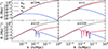 |
Fig. 1. Velocity divergence θ for dark energy (blue), dark matter (red), and non-interacting baryons (black) for different values of the coupling parameter α. For the case analysed here, with α = 1, we can corroborate that the velocity of dark energy is much lower than those of baryons and dark matter, thereby justifying the approximation vdm ≫ vde and vb ≫ vde, i.e. neglecting dark energy velocities on the scales relevant to our simulations. |
where L is the comoving size of the simulation box in Mpc/h and H0 is the Hubble constant. Therefore, since the time evolution of the dark matter energy density remains unmodified, we only need to rewrite the velocity into super-comoving coordinates, as displayed above. However, not all particles should have their velocities updated by the extra elastic interacting term. Consequently, to properly distinguish particles subject to the interaction (dark matter) from those that are not (baryons), we introduced a ‘family’ category for the particles in the simulation. Each particle is labelled either as dark matter – experiencing the additional term in Equation (16) – or as baryons, which do not experience the momentum transfer term. To ensure consistency, the relative number of particles assigned to each family follows the cosmology used, matching in particular the proportions given by the values of Ωb and Ωdm provided below.
4. Results from the simulations
In this work, we consider a cosmology described by the following parameters: the Hubble parameter H0 = 67.7 km/s/Mpc, today’s density parameters Ωb = 0.045, Ωdm = 0.269, scalar perturbations As = 2.1 × 10⁻⁹ and ns = 0.968, and dark energy equation-of-state w = −0.98. The initial conditions were obtained from the MUSIC2-monofonIC code Hahn et al. (2020, 2021) using its default settings and, in particular, the third-order Lagrangian perturbation theory (3LPT) with the aforementioned parameters, where the required transfer function was generated by the Boltzmann solver CLASS Blas et al. (2011). The analyses were performed for a box with L = 103 Mpc/h, populated with N = 5123 particles. We performed two simulations:
-
one with the ΛCDM model using the aforementioned cosmological parameters.
-
another with the covariantised dark Thomson-like scattering model using the same cosmological parameters as well as a coupling parameter α = 1. The initial conditions for this simulation were the same as those for the ΛCDM one, justified by the interaction’s irrelevance at the initial condition time. Additionally, only dark matter particles evolved according to equation (16), while baryon particles followed the standard evolution given by equation (14).
We now proceed to analyse the results from our simulations. In particular, we compare them with the ΛCDM case in order to assess the impact of the interaction on non-linear scales.
4.1. Matter power spectrum and check with linear results
In Figure 2, we present the evolution of the matter power spectrum at various redshifts, while in Figure 3 we show the same redshift evolution but for the relative difference between the matter power spectrum in the interacting case and the reference ΛCDM model. With the exception of very large scales k ≲ (aH)0, where our numerical implementation is expected to produce unreliable results2, the primary effects of the interaction are mostly observed on non-linear scales and only become significant at relatively late cosmic times. This behaviour is consistent with the results obtained from linear perturbation theory.
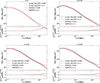 |
Fig. 2. Matter power spectrum at different redshifts, computed using the modified version of CLASS with HALOFIT and from RAMSES (upper panels), and the ratio P(k)HALOFIT/P(k)RAMSES − 1 (lower panels), illustrating the precision with which HALOFIT predicts non-linear scales. |
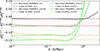 |
Fig. 3. Relative matter power spectra differences between the covariantised dark Thomson-like interacting model and the ΛCDM model at different redshifts, computed from the simulation output using all particles (solid lines) and the linear solver CLASS (dash-dotted lines). |
At redshift z = 1, shown in the first panel, no noticeable deviation is observed between the standard cosmological model and the interacting scenario. Although already known from previous studies (see Asghari et al. 2019; Beltrán Jiménez et al. 2021b; Cardona & Figueruelo 2022; Beltrán Jiménez et al. 2024), this supports our use of the same initial conditions for both ΛCDM and the interacting model simulations. However, as the interaction affects evolution when Γ ≳ ℋ, its influence first manifests on smaller scales, as apparent in the second panel at redshift z = 0.42. The effect reduces clustering since momentum transfer prevents dark matter from efficiently falling into gravitational potential wells. As cosmic evolution progresses and the interaction further intensifies, the range of affected scales expands towards larger scales. This increasing drag impact suppresses structure formation, reflected in reduced clustering amplitude on a wider range of scales. Consequently, the matter power spectrum in the interacting scenario with α = 1 exhibits a systematically lower amplitude than the standard cosmological model on smaller scales. This trend is in full agreement with previous results derived from the linear regime, as seen by comparing the results from the CLASS Boltzmann solver using the HALOFIT non-linear prescription Lesgourgues (2011), Blas et al. (2011). We can, however, see that HALOFIT underestimates suppression on small scales. This agrees with the expectation in Laguë et al. (2024) where the authors developed a halo-model approach to include quasi-linear scales in the elastic interacting model (wΓCDM) considered in this work. The authors expect HALOFIT to underestimate the impact of the interaction in the non-linear regime, and our full N-body simulations confirm this expectation.
Finally, at highly non-linear scales, we observe an increase in the power spectrum, indicating enhanced dark matter clustering from the elastic interaction. This effect opposes the expected suppression of structures induced by the interaction by naively extrapolating the results of the linear scales. One may be tempted to ascribe this effect to a numerical issue related to the resolution of the simulations, but Figure 4 clearly shows that it is driven by dark matter and is, thus, physical. A similar effect has also been observed in Baldi & Simpson (2015, 2017) for the elastic scattering scenario between the dark energy and dark matter introduced in Simpson (2010). These studies nicely explain how enhanced clustering can be understood in terms of non-linear virialisation. On non-linear scales where dark matter particles acquire angular momentum, the interaction catalyses kinetic energy loss that modifies virialisation. Having less kinetic energy, the virialised structure shrinks with respect to the non-interacting case and causes a more clustered matter distribution. This explanation is later confirmed in section 4.3, where we study the dark matter halo profiles under the model and find that structures indeed shrink due to the interaction. Analogous results were also found in a similar scenario with pure momentum exchange between dark matter and quintessence dark energy in Palma & Candlish (2023), Candlish & Jaffé (2025).
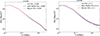 |
Fig. 4. Matter power spectrum for the ΛCDM model (left) and for the covariantised dark Thomson-like interacting model at z = 0.05, computed from the simulation output using all particles (black dots), dark matter particles (blue line), and baryons particles (red line). |
The simulations in Baldi & Simpson (2015) consider dark matter only, while we have also included a non-interacting component as a proxy for baryons to study their response. This is shown in Figure 4 where we can see how enhanced clustering on non-linear scales is substantially more pronounced for interacting DM, while baryons remain only mildly sensitive to the effect because they feel it only through the modification to the gravitational potential. In the halo-model based on the spherical collapse of Laguë et al. (2024), an increase in the power spectrum likewise found on small scales was attributed to mode-coupling to large-scale modes. While their results are expected to be valid only on quasi-linear scales, our results show that this trend extends to fully non-linear scales. Let us finally note that the enhanced power spectrum on non-linear scales has also been observed in Ferlito et al. (2022) simulations of elastic scattering between dark energy and baryons. The effect found in that work is however milder for two reasons: baryons are less abundant than dark matter, and the interaction rate from elastic Thomson scattering decreases with expansion.
4.2. Halos: Global picture
We now turn our attention to how different halos form and are distributed. To analyse this, we used MatchMaker3, a friend-of-friend halo finder, with standard parameters: a linking length of bfof = 0.2 in mean inter-particle distance units and a minimum of nmin = 20 particles per halo. Since we focus on the overall behaviour, we do not distinguish between dark matter and baryon particles when identifying halos, though it is important to note that the interaction does differentiate the two, as later analysed. With these considerations in mind, Figure 5 shows the spatial distribution of the halos detected by MatchMaker. Each dot represents an individual halo, and the colour and size of the dots correspond to the halo mass, measured in units of M⊙/h. Comparing the result from the ΛCDM and the interacting model simulations, we can already see how the interaction suppresses the formation of very massive halos, while medium and small mass halos seem insensitive in terms of their abundance. Since halo formation is a hierarchical process in the CDM paradigm, we know that those very massive halos form only at very late times and from the merging of smaller halos. Therefore, as the momentum transfer for α = 1 occurs only at low redshift, it is natural that the most massive halos are those prevented from forming. In other words, the most massive halos – those forming when the interaction becomes efficient, Γ ≳ ℋ – are affected by the clustering deficit of the interacting model. On the other hand, from our analyses we can finally infer that the momentum transfer does not disrupt already formed structures but only halts the accretion process, preventing further growth of density perturbations.
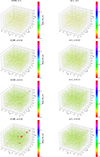 |
Fig. 5. Spatial distribution of the halos found. Each dot represents a halo, whose colour and dot-size are proportional to the halo mass. |
To explore the formation of halos in more detail, we perform a halo number count analysis. In Figure 6, we present the number of halos formed as a function of their mass. The differences between the ΛCDM model and the interacting scenario are not statistically significant for lower-mass halos. Again, these halos typically form when the interaction becomes effective. Thus, we can now quantitatively conclude that the number of smaller and medium-sized halos formed is insensitive to this interaction. The mass scale where the halos are affected is fixed by the same parameter that controls the strength of the interaction, α, since it also controls the timescale at which the interaction becomes efficient. For halos larger than that scale, significant differences emerge. At early times such as z = 1, when the interaction has yet to take effect, no differences are observed. This is expected, as both scenarios begin with the same initial conditions and follow similar evolutionary histories, leading to identical early structure formation in both simulated Universes. Once the interaction becomes efficient, however, the formation of very massive halos is suppressed in the momentum transfer simulation. This trend aligns with the patterns observed in the spatial distribution of the halos. We can conclude that only the most massive ones forming at the onset of the interaction are significantly affected in terms of structure formation. Furthermore, this modification manifests as a reduced formation probability, ultimately resulting in a Universe with fewer very massive structures.
 |
Fig. 6. Halo mass distribution in M⊙/h for the standard model (black) and the covariantised dark Thomson-like interaction (red). |
4.3. Halos: Individual picture
In the previous section, we discussed how the momentum transfer induced by the elastic interaction results in a noticeable suppression of very massive halos compared to a non-interacting scenario. However, the impact of the interaction on the formation of individual halos still requires a detailed assessment. This issue is addressed below.
In Figure 7, we present the averaged radial density profiles of a representative sample of the same halos found in both the ΛCDM scenario (black line) and the covariantised dark Thomson-like interacting model (red line). Let us recall that both simulations start from the same initial conditions, and that the clustering process evolves identically up to the onset of the strong elastic interaction epoch. Thus, a population of analogous halos that form at similar positions in both simulations. These are the halos we compare here in order to study the interaction effects on the halo profile. The selected halos are divided into two different mass scales from the reference non-interacting case to facilitate visualization: Mhalo ∼ 1015 M⊙/h (left panel) and Mhalo ∼ 1014 M⊙/h (right panel). These plots allow us to directly compare the internal halo structures under both scenarios. Furthermore, we used the critical density of the Universe today ρcr to normalise the radial density of each halo.
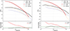 |
Fig. 7. Top panels: Stacked radial density profiles for a sample of 40 halos identified as the same in both the ΛCDM simulation (black-blue lines) and the covariantised dark Thomson-like interacting model simulation (red-orange lines). We show the total (solid lines), dark matter (dashed lines), and baryonic (dotted lines) density profiles. Bottom panels: Ratio between the dark matter and baryon density profiles for the ΛCDM (black lines) and the covariantised dark Thomson-like interacting model (red lines) simulations versus the reference ratio Ωdm/Ωb (dashed green line). We show the results for two different halo masses with reference to the non-interacting case: Mhalo ∼ 1015 M⊙/h (left panel) and Mhalo ∼ 1014 M⊙/h (right panel). Since we started from the same initial conditions, we identify each halo by its formation at the same spatial position and similar mass range, taking into account that the covariantised dark Thomson-like scattering produces less massive halos. |
From the resulting density profiles, the halos interestingly appear more compact and smaller in the interacting case compared to their counterparts in the standard ΛCDM scenario. The halo cores formed in the interacting model feature significantly higher central densities, suggesting more concentrated mass distributions due to the interaction. This picture is further supported by the fact that the radial density distribution declines more steeply in the interacting model, resulting in less massive and more diffuse outer regions of the halos. These results are in agreement with the explanation given above for the power spectrum enhancement on non-linear scales, i.e. that the interaction reduces the kinetic energy of dark matter particles in virialised objects, making them more compact. We also see in Figure 7 how the baryon profile is slightly less compact. Although they do not interact directly with dark energy, they feel a reduced gravitational potential – an effect more prominent for more massive halos. We note that a distinctive signature of the interacting model is precisely the different dark matter and baryon profiles shown in the lower panels. A consequence of having different baryon and dark matter profiles is that the standard spherical collapse model – where the mass within each shell is conserved – fails earlier than in the standard case. In other words, shell-crossing occurs earlier than expected in a pure ΛCDM. With this in mind, it may be interesting to revisit the halo-model – based on spherical collapse for quasi-linear scales of Laguë et al. (2024) – with a more complete spherical collapse model that includes baryons (as an additional collisionless, non-interacting component) and accounts for shell crossings from both components. This setup with two matter components – one of which features an interaction that modifies spherical collapse – resembles the scenarios with charged dark matter studied in Beltrán Jiménez et al. (2021a). Hence, we may expect some qualitative similarities.
While in the non-interacting case both dark matter and baryon profiles scale equally with distance, the interacting scenario shows enhancement in the radial density of dark matter in the innermost shells of the halos in comparison with baryons, with lighter outskirts. This observation is consistent with our previous results. The interaction, which only couples to dark matter, inhibits the accretion of dark matter particles at late times. During halo formation, this effect primarily impacts their outer regions. Consequently, when the interaction becomes efficient at late times, dark matter accretion nearly ceases, whereas baryons continue to fall into weakened gravitational potential wells. It is noteworthy that this particular effect extends to halos of all scales, rather than being limited to the most massive ones, as observed in previous effects. Therefore, the momentum transfer interactions seem to sweep the outskirts of the halo of dark matter particles.
A final conclusion from these results is the following: in momentum transfer scenarios of this type, using baryon profiles as templates for the underlying dark matter field within individual halos introduces an additional radially dependent bias. However, the central question remains whether baryons can still serve as reliable tracers of the overall density field – or, in other words, whether galaxies will continue to reside at the bottom of dark matter potential wells. This is confirmed in the following section through an analysis of the cosmic web.
4.4. Cosmic web
We now turn our attention to how the elastic interaction alters the cosmic web. Given that momentum transfer occurs exclusively in the dark matter component and not in baryons, a key issue is whether both matter components remain interconnected. In particular, in relation to observations, it is important to assess whether galaxies continue to serve as reliable tracers of the dark matter velocity field and whether they remain located at the bottom of dark matter potential wells.
In Figure 8, we show dark matter distribution as a density field ranging from black (representing lower dark matter density) to blue (indicating high concentrations of dark matter) for our cosmological parameters and fiducial coupling parameter α = 1. Overlaid on this, we also illustrate iso-density regions of high baryon concentration with yellow isogram lines, which mark the contours of constant baryon density. Contours corresponding to lower baryon densities are omitted for visualisation purposes. These contours effectively highlight the densest clumps of baryons in our simulations, corresponding to the locations where galaxies will reside. A weakening of the cosmic web is evident, as dark matter exhibits significantly reduced clustering in the interacting case than in the standard scenario. Furthermore, we note that regions of very high density, both massive halo nodes and connecting filaments, appear more compact, reinforcing our previous analyses of how the elastic interaction clears dark matter particles from the surrounding areas of a halo, where accretion occurs in the standard scenarios.
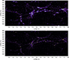 |
Fig. 8. Matter distribution for the ΛCDM (top) and the interacting αCDM (bottom) models. Dark matter is represented by the black-blue-green gradient density map, while high-density baryon regions are represented by yellow contours. We confirm that the interaction gives rise to a less clustered universe and that the baryons remain locked inside the dark matter halos. |
Regarding whether baryons remain tracers of dark matter, Figure 8 shows that baryons – which we take as proxies for galaxies in the simulations – remain gravitationally bound to dark matter halos. Galaxies mainly form prior to the onset of elastic interaction dominance. Once formed and virialised at the bottom of the potential wells shaped by dark matter halos, they remain attached to these structures, even though the interaction inhibits further halo growth. Baryon halos, our galaxies proxies, and their host halos constitute strongly bound systems. For reasonable values of the coupling parameter, they show no disassembly from elastic interaction as seen in the Figure 8. Taken together with our previous results from the matter distribution, we conclude that the overall distribution of baryons remains largely unaffected and still serve as a proxy for where galaxies will form. While the profile analyses suggest the baryon halos will change due to the interaction, this implies galaxy formation will be modified. However, we must note that galaxies typically form and virialise before the onset of elastic interaction, and that their formation process is more complicated in our simulation, where we simply assigned some particles as baryons. Thus, we conclude that once formed they will inhabit shallower dark matter potential wells due to the effect of the interaction on the surrounding dark matter distribution. As a consequence, their accretion process will be reduced, resulting in more compact objects, although the effect is milder than in the case of dark matter halos.
5. Discussion
In this work, we explored the non-linear regime of a particular example of pure momentum transfer interactions in the dark sector, the so-called covariantised dark Thomson-like scattering between dark energy and dark matter. We studied a fiducial model with the coupling parameter set to α = 1, which corresponds to the best-fit value obtained from cosmological probes in previous studies. The main goal here was to explore small scales corresponding to the non-linear regime of structure formation. To this aim, we implemented the model into the RAMSES code and performed two simulations, one for the standard ΛCDM scenario and the other for our interacting model. Furthermore, we exploited the late onset of the interacting epoch to set identical initial conditions for both simulations, since the interaction is negligible at the initial redshift. This further means that noticeable effects only emerge at low redshift. The simulations show that the elastic interaction suppresses the matter power spectrum at very late times and small scales compared to ΛCDM. Thus, our results extend the clustering suppression observed in previous studies on linear scales to the non-linear regime and confirms the expected behaviour.
We also analysed halo formation in the elastic interacting scenario. We observe that very massive halos are significantly less likely to form in the standard ΛCDM scenario, while less massive halos remain essentially unaffected in the amount formed. This feature was confirmed both by studying the halo particle distribution and the total mass distribution of the halos in the simulations. This reflects that the most massive halos are the last to form in the hierarchical structure formation paradigm. They are thus most affected by the interaction, which becomes efficient only at late times. We must remember here that the interaction’s only new parameter, α, sets the timescale for when the interaction becomes efficient. Therefore, α also controls the threshold mass above which the number of halos decreases. For the case studied here (α = 1), this corresponds to masses around 2 × 10¹⁴ M⊙/h at z = 0.05. Higher α values affect lighter halos, and vice versa for lower values. Thus, once elastic interaction dominates, the most massive structures at that moment will not merge or accrete, as is otherwise the case. Less massive halos, on the other hand, already formed prior to the interacting epoch in accordance with the hierarchical formation process of halo formation. Since the interaction is unable to disrupt halos which already formed, their abundance is insensitive to the interaction.
On the other hand, when analysing the internal dynamics of individual halos, we find that they undergo a noticeable increase in the steepness of their profiles. This implies that halos are more compact objects with shorter radial extension. This effect is particularly prominent in the coupled component, dark matter, which becomes increasingly concentrated in the inner regions of the halos, while the outskirts are emptied as the interaction suppresses further accretion. Driven by this effect, baryons also suffer a similar but milder compactification of their profiles. Furthermore, inner layers of the halos show a significant enrichment of dark matter, while the outer layers contain a larger proportion of baryons than in ΛCDM. This occurs because the interaction prevents dark matter accretion into the potential wells but does not affect baryons. We note here that this effect, although more prominent in larger halos, affects all halos, unlike the reduction in halo formation, which affects only the most massive halos forming when the interaction becomes efficient. As a consequence, when tracing the underlying matter distribution with baryons, we must account for an additional bias on halo scales.
Finally, we analysed how faithfully baryons trace the dark matter distribution. Although the interaction weakens the growth of structures in both filaments and nodes, we find that high baryon density regions, which we assume to be a proxy for the location of galaxies, show a significant overlap with dark matter overdensities. This result suggests that baryons remain good tracers of the dark matter density field in the presence of the elastic interaction.
Recently, the interacting model considered in this work was tested against the latest ACT data in Calabrese et al. (2025) using a model of the non-linear regime developed in Laguë et al. (2024)4. This non-linear modelling is based on a modified spherical collapse model on quasi-linear scales to obtain the critical overdensity for the elastic interacting model, plus implementation in HMCode Mead et al. (2021). The N-body code developed in this paper will allow to test the validity of the method developed in Laguë et al. (2024) and used in Calabrese et al. (2025). Moreover, it will allow us to go beyond quasi-linear scales. Incorporating other datasets in a fully consistent way requires good modelling of the non-linear scales lacking in the literature. Our developed N-body code and our set of simulations fill this gap. These will enable more appropriate confrontation with data and assessment of the extent to which current data favor elastic interaction. In this respect, Doux & Karwal (2026) have explored a scale-dependent modification of the power spectrum. It showed that galaxy-lensing data from DESY3 Doux et al. (2022), KiDS-1000 Asgari et al. (2021), HSC Y3 Dalal et al. (2023), and ACT DR6 Madhavacheril et al. (2024), Qu et al. (2024) prefer a 15-30% suppression in the power spectrum compared to Planck results. Since ACT lensing is consistent with Planck under ΛCDM and its sensitivity peaks at around z ≃ 2, this further supports the idea that the effects may come from intermediate and/or small scales at low redshift (see discussion in e.g. Beltrán Jiménez et al. (2025)). The results of Doux & Karwal (2026) rely on HALOFIT which, in principle, may not be justified, but our results show that it indeed gives a reasonably good description of the non-linear regime. On the other hand, it is interesting to note that the method developed in Doux & Karwal (2026) assumes a fixed background cosmology. This makes elastic scenarios such as the one considered here particularly well-suited since the background remains unaltered by construction. On the other hand, the scale-dependent modification of the power spectrum of the elastic model depends on redshift and would need to be included in Doux & Karwal (2026)’s method. Given the simplicity of the elastic interaction effects, we expect their inclusion to be straightforward.
In conclusion, with these results we tested the momentum transfer scenarios by checking the differences and assumptions in structure formation in the Universe, particularly for upcoming weak lensing and galaxy-clustering data probes. Despite the extreme simplicity of this scenario with the addition of only one new parameter, these results also show that effects appear from halo formation to global clustering; therefore, forthcoming experiments will be able to constrain momentum transfer models. An exhaustive exploitation of data from surveys such as Euclid Laureijs et al. (2011), DES The Dark Energy Survey Collaboration (2005), DESI DESI Collaboration (2016), and J-PAS Benitez et al. (2014) requires comprehensive knowledge of non-linear clustering to reliably extract information from the data5. This will become even more important for the next generation of stage-five experiments (see e.g. Besuner et al. 2025). This work represents a first step in this direction. Future work will refine our results with higher resolution and complete simulations as well as analyse other promising observables to test the elastic interacting model. In this respect, it will be interesting to analyse velocity correlations since the interaction precisely depends on the peculiar velocities of dark matter. Another interesting observable would be void properties. It Schuster et al. (2025) recently pointed out that the evolution of voids in ΛCDM stabilises at z ≃ 1 – the redshift at which the elastic interaction becomes relevant according to the obtained constraints in previous studies Figueruelo et al. (2021). Thus, we may expect elastic interaction to generate further evolution of voids below z = 1, which could provide another distinctive signature of these scenarios.
Acknowledgments
JBJ thanks the Institute of Theoretical Astrophysics of the University of Oslo for the hospitality and excellent environment provided during the completion of this work. JBJ acknowledges support from Projects PID2021-122938NB-I00 and PID2024-158938NB-I00 funded by MICIU/AEI/10.13039/501100011033 and by “ERDF A way of making Europe”, the Project SA097P24 funded by Junta de Castilla y León and the research visit grant PRX23/00530. DF acknowledged support from “Convocatoria de contratación de personal investigador doctor de la UPV/EHU (2024)”. DF acknowledged support by the Grant PID2021-123226NB-I00 (funded by MCIN/AEI/10.13039/501100011033 and by “ERDF A way of making Europe") and by the Grant PID2024-158938NB-I00 (funded by MICIU/AEI/ 10.13039/501100011033 and by “ERDF A way of making Europe”). We thank the Research Council of Norway for their support and the resources provided by UNINETT Sigma2 – the National Infrastructure for High-Performance Computing and Data Storage in Norway. This article is also based upon work from COST Action CA21136 Addressing observational tensions in cosmology with systematics and fundamental physics (CosmoVerse) supported by COST (European Cooperation in Science and Technology).
References
- Abdalla, E., Abellán, G. F., Aboubrahim, A., et al. 2022, JHEAp, 34, 49 [NASA ADS] [Google Scholar]
- Abdul Karim, M., Aguilar, J., Ahlen, S., et al. 2025, Phys. Rev. D, 112, 083515 [Google Scholar]
- Alam, S., Aubert, M., Avila, S., et al. 2021, Phys. Rev. D, 103, 083533 [NASA ADS] [CrossRef] [Google Scholar]
- Amendola, L., & Tsujikawa, S. 2020, JCAP, 06, 020 [Google Scholar]
- Anderson, L., Aubourg, E., Bailey, S., et al. 2013, MNRAS, 427, 3435 [Google Scholar]
- Aoki, K., Beltrán Jiménez, J., Pookkillath, M. C., & Tsujikawa, S. 2025, arXiv e-prints [arXiv:2504.17293] [Google Scholar]
- Asgari, M., Lin, C.-A., Joachimi, B., et al. 2021, A&A, 645, A104 [NASA ADS] [CrossRef] [EDP Sciences] [Google Scholar]
- Asghari, M., Beltrán Jiménez, J., Khosravi, S., & Mota, D. F. 2019, JCAP, 04, 042 [Google Scholar]
- Baldi, M., & Simpson, F. 2015, MNRAS, 449, 2239 [NASA ADS] [CrossRef] [Google Scholar]
- Baldi, M., & Simpson, F. 2017, MNRAS, 465, 653 [CrossRef] [Google Scholar]
- Beltrán Jiménez, J., Bettoni, D., Figueruelo, D., & Teppa Pannia, F. A. 2020, JCAP, 08, 020 [Google Scholar]
- Beltrán Jiménez, J., Bettoni, D., & Brax, P. 2021a, Phys. Rev. D, 103, 103505 [Google Scholar]
- Beltrán Jiménez, J., Bettoni, D., Figueruelo, D., Teppa Pannia, F. A., & Tsujikawa, S. 2021b, Phys. Rev. D, 104, 103503 [Google Scholar]
- Beltrán Jiménez, J., Di Dio, E., & Figueruelo, D. 2023, JCAP, 11, 088 [Google Scholar]
- Beltrán Jiménez, J., Figueruelo, D., & Teppa Pannia, F. A. 2024, Phys. Rev. D, 110, 023527 [Google Scholar]
- Beltrán Jiménez, J., Bettoni, D., Figueruelo, D., & Teppa Pannia, F. A. 2025, Phys. Dark Univ., 47, 101761 [Google Scholar]
- Benitez, N., Dupke, R., Moles, M., et al. 2014, arXiv e-prints [arXiv:1403.5237] [Google Scholar]
- Besuner, R., Dey, A., Drlica-Wagner, A., et al. 2025, arXiv e-prints [arXiv:2503.07923] [Google Scholar]
- Betoule, M., Kessler, R., Guy, J., et al. 2014, A&A, 568, A22 [NASA ADS] [CrossRef] [EDP Sciences] [Google Scholar]
- Beutler, F., Blake, C., Colless, M., et al. 2011, MNRAS, 416, 3017 [NASA ADS] [CrossRef] [Google Scholar]
- Blas, D., Lesgourgues, J., & Tram, T. 2011, JCAP, 2011, 034 [Google Scholar]
- Calabrese, E., Colin Hill, J., Jense, H. T., et al. 2025, JCAP, 11, 063 [Google Scholar]
- Candlish, G. N., & Jaffé, Y. L. 2025, A&A, 703, A38 [NASA ADS] [CrossRef] [EDP Sciences] [Google Scholar]
- Cardona, W., & Figueruelo, D. 2022, JCAP, 12, 010 [Google Scholar]
- Cardona, W., Palacios-Córdoba, J. L., & Valenzuela-Toledo, C. A. 2024, JCAP, 04, 016 [Google Scholar]
- Chamings, F. N., Avgoustidis, A., Copeland, E. J., Green, A. M., & Pourtsidou, A. 2020, Phys. Rev. D, 101, 043531 [Google Scholar]
- Cruickshank, N., Crittenden, R., Koyama, K., & Bruni, M. 2025, JCAP, 10, 052 [Google Scholar]
- Dalal, R., Li, X., Nicola, A., et al. 2023, Phys. Rev. D, 108, 123519 [CrossRef] [Google Scholar]
- De Felice, A., Nakamura, S., & Tsujikawa, S. 2020, Phys. Rev. D, 102, 063531 [Google Scholar]
- DES Collaboration (Abbott, T. M. C., et al.) 2022, Phys. Rev. D, 105, 023520 [CrossRef] [Google Scholar]
- DESI Collaboration (Aghamousa, A., et al.) 2016, arXiv e-prints [arXiv:1611.00036] [Google Scholar]
- Di Valentino, E., Said, J. L., Riess, A., et al. 2025, Phys. Dark Univ., 49, 101965 [Google Scholar]
- Doux, C., & Karwal, T. 2026, Open J. Astrophys., 9, 155045 [Google Scholar]
- Doux, C., Jain, B., Zeurcher, D., et al. 2022, MNRAS, 515, 1942 [Google Scholar]
- Ferlito, F., Vagnozzi, S., Mota, D. F., & Baldi, M. 2022, MNRAS, 512, 1885 [CrossRef] [Google Scholar]
- Figueruelo, D., Resco, M. A., Teppa Pannia, F. A., et al. 2021, JCAP, 07, 022 [Google Scholar]
- Hahn, O., Michaux, M., Rampf, C., Uhlemann, C., & Angulo, R. E. 2020, Astrophysics Source Code Library [record ascl:2008.024] [Google Scholar]
- Hahn, O., Rampf, C., & Uhlemann, C. 2021, MNRAS, 503, 426 [NASA ADS] [CrossRef] [Google Scholar]
- Heymans, C., Grocutt, E., Alan, H., et al. 2013, MNRAS, 432, 2433 [Google Scholar]
- Kase, R., & Tsujikawa, S. 2020, Phys. Lett. B, 804, 135400 [Google Scholar]
- Koivisto, T. S., Saridakis, E. N., & Tamanini, N. 2015, JCAP, 09, 047 [CrossRef] [Google Scholar]
- Kumar, S., & Nunes, R. C. 2017, Eur. Phys. J. C, 77, 734 [Google Scholar]
- Laguë, A., McCarthy, F., Madhavacheril, M., Hill, J. C., & Qu, F. J. 2024, Phys. Rev. D, 110, 023536 [Google Scholar]
- Laureijs, R., Amiaux, J., Arduini, S., et al. 2011, arXiv e-prints [arXiv:1110.3193] [Google Scholar]
- Lesgourgues, J. 2011, arXiv e-prints [arXiv:1104.2932] [Google Scholar]
- Linton, M. S., Crittenden, R., & Pourtsidou, A. 2022, JCAP, 08, 075 [Google Scholar]
- Madhavacheril, M. S., Qu, F. J., Sherwin, B. D., et al. 2024, ApJ, 962, 113 [CrossRef] [Google Scholar]
- Mancini Spurio, A., & Pourtsidou, A. 2022, MNRAS, 512, L44 [Google Scholar]
- Martel, H., & Shapiro, P. R. 1998, MNRAS, 297, 467 [Google Scholar]
- Mead, A., Brieden, S., Tröster, T., & Heymans, C. 2021, MNRAS, 502, 1401 [Google Scholar]
- Nakamura, S., Kase, R., & Tsujikawa, S. 2019, JCAP, 12, 032 [Google Scholar]
- Palma, D., & Candlish, G. N. 2023, MNRAS, 526, 1904 [NASA ADS] [Google Scholar]
- Perivolaropoulos, L., & Skara, F. 2022, New Astron. Rev., 95, 101659 [CrossRef] [Google Scholar]
- Planck Collaboration V. 2020, A&A, 641, A5 [NASA ADS] [CrossRef] [EDP Sciences] [Google Scholar]
- Planck Collaboration VI. 2020, A&A, 641, A6 [NASA ADS] [CrossRef] [EDP Sciences] [Google Scholar]
- Planck Collaboration XXIV. 2016, A&A, 594, A24 [NASA ADS] [CrossRef] [EDP Sciences] [Google Scholar]
- Pookkillath, M. C., & Koyama, K. 2024, JCAP, 10, 105 [Google Scholar]
- Poulin, V., Bernal, J. L., Kovetz, E. D., & Kamionkowski, M. 2023, Phys. Rev. D, 107, 123538 [NASA ADS] [CrossRef] [Google Scholar]
- Pourtsidou, A., & Tram, T. 2016, Phys. Rev. D, 94, 043518 [CrossRef] [Google Scholar]
- Pourtsidou, A., Skordis, C., & Copeland, E. J. 2013, Phys. Rev. D, 88, 083505 [NASA ADS] [CrossRef] [Google Scholar]
- Qu, F. J., Sherwin, B. D., Madhavacheril, M. S., et al. 2024, ApJ, 962, 112 [NASA ADS] [CrossRef] [Google Scholar]
- Ross, A. J., Samushia, L., Howlett, C., et al. 2015, MNRAS, 449, 835 [NASA ADS] [CrossRef] [Google Scholar]
- Schuster, N., Hamaus, N., Pisani, A., Dolag, K., & Weller, J. 2025, arXiv e-prints [arXiv:2509.07092] [Google Scholar]
- Simpson, F. 2010, Phys. Rev. D, 82, 083505 [NASA ADS] [CrossRef] [Google Scholar]
- Skordis, C., Pourtsidou, A., & Copeland, E. J. 2015, Phys. Rev. D, 91, 083537 [NASA ADS] [Google Scholar]
- Teyssier, R. 2002, A&A, 385, 337 [CrossRef] [EDP Sciences] [Google Scholar]
- The Dark Energy Survey Collaboration (Abbott, T., et al.) 2005, arXiv e-prints [arXiv:astro-ph/0510346] [Google Scholar]
- Vagnozzi, S., Visinelli, L., Mena, O., & Mota, D. F. 2020, MNRAS, 493, 1139 [Google Scholar]
For Thomson scattering, the timescale when the interaction was efficient is in the early Universe, when the pressure-bearing component – photons – was non-negligible.
On very large scales, dark energy velocity becomes comparable to that of matter, so our approximation vdm ≫ vde and vb ≫ vde breaks down. Since we are interested in small (non-linear) scales, this is not relevant for our purposes here. However, this should be refined for simulations that include relativistic effects and/or when effects of near horizon scales are analysed.
MatchMaker is available at https://github.com/damonge/MatchMaker.
In Calabrese et al. (2025) and Laguë et al. (2024), the elastic scattering model of Simpson (2010) is considered, although these studies actually employ the covariantised model used here. As explained above, while both scenarios formally give identical linear perturbation equations, proper Thomson scattering dominates at high redshift, whereas the covariantised interacting model becomes more relevant at low redshift.
For instance, the recent forecast analysis performed in Cruickshank et al. (2025) for the scenario studied in this work, but with a redshift-dependent interacting parameter, could be refined to include some quasi-linear or non-linear scales in a robust way.
All Figures
|
Fig. 1. Velocity divergence θ for dark energy (blue), dark matter (red), and non-interacting baryons (black) for different values of the coupling parameter α. For the case analysed here, with α = 1, we can corroborate that the velocity of dark energy is much lower than those of baryons and dark matter, thereby justifying the approximation vdm ≫ vde and vb ≫ vde, i.e. neglecting dark energy velocities on the scales relevant to our simulations. |
| In the text | |
|
Fig. 2. Matter power spectrum at different redshifts, computed using the modified version of CLASS with HALOFIT and from RAMSES (upper panels), and the ratio P(k)HALOFIT/P(k)RAMSES − 1 (lower panels), illustrating the precision with which HALOFIT predicts non-linear scales. |
| In the text | |
|
Fig. 3. Relative matter power spectra differences between the covariantised dark Thomson-like interacting model and the ΛCDM model at different redshifts, computed from the simulation output using all particles (solid lines) and the linear solver CLASS (dash-dotted lines). |
| In the text | |
|
Fig. 4. Matter power spectrum for the ΛCDM model (left) and for the covariantised dark Thomson-like interacting model at z = 0.05, computed from the simulation output using all particles (black dots), dark matter particles (blue line), and baryons particles (red line). |
| In the text | |
|
Fig. 5. Spatial distribution of the halos found. Each dot represents a halo, whose colour and dot-size are proportional to the halo mass. |
| In the text | |
|
Fig. 6. Halo mass distribution in M⊙/h for the standard model (black) and the covariantised dark Thomson-like interaction (red). |
| In the text | |
|
Fig. 7. Top panels: Stacked radial density profiles for a sample of 40 halos identified as the same in both the ΛCDM simulation (black-blue lines) and the covariantised dark Thomson-like interacting model simulation (red-orange lines). We show the total (solid lines), dark matter (dashed lines), and baryonic (dotted lines) density profiles. Bottom panels: Ratio between the dark matter and baryon density profiles for the ΛCDM (black lines) and the covariantised dark Thomson-like interacting model (red lines) simulations versus the reference ratio Ωdm/Ωb (dashed green line). We show the results for two different halo masses with reference to the non-interacting case: Mhalo ∼ 1015 M⊙/h (left panel) and Mhalo ∼ 1014 M⊙/h (right panel). Since we started from the same initial conditions, we identify each halo by its formation at the same spatial position and similar mass range, taking into account that the covariantised dark Thomson-like scattering produces less massive halos. |
| In the text | |
|
Fig. 8. Matter distribution for the ΛCDM (top) and the interacting αCDM (bottom) models. Dark matter is represented by the black-blue-green gradient density map, while high-density baryon regions are represented by yellow contours. We confirm that the interaction gives rise to a less clustered universe and that the baryons remain locked inside the dark matter halos. |
| In the text | |
Current usage metrics show cumulative count of Article Views (full-text article views including HTML views, PDF and ePub downloads, according to the available data) and Abstracts Views on Vision4Press platform.
Data correspond to usage on the plateform after 2015. The current usage metrics is available 48-96 hours after online publication and is updated daily on week days.
Initial download of the metrics may take a while.