| Issue |
A&A
Volume 707, March 2026
|
|
|---|---|---|
| Article Number | A114 | |
| Number of page(s) | 9 | |
| Section | Planets, planetary systems, and small bodies | |
| DOI | https://doi.org/10.1051/0004-6361/202558305 | |
| Published online | 10 March 2026 | |
The dependence of asteroid rotation on composition
A spectral class database for MP3C
1
Université Côte d’Azur, CNRS-Lagrange, Observatoire de la Côte d’Azur,
CS 34229,
06304
Nice Cedex 4,
France
2
University of Leicester, School of Physics and Astronomy,
University Road,
LE1 7RH
Leicester,
UK
3
JSPS International Research Fellow, Department of Earth and Planetary Science, The University of Tokyo,
Tokyo,
Japan
4
Institute for Astronomy, Astrophysics, Space Applications and Remote Sensing, National Observatory of Athens,
Metaxa & Vas. Pavlou St.,
15236
Penteli, Athens,
Greece
5
Charles University, Faculty of Mathematics and Physics, Institute of Astronomy,
V Holešovičkách 2,
180 00
Prague,
Czech Republic
6
Astronomical Institute, Academy of Sciences of the Czech Republic,
Fričova 298,
Ondřejov
25165,
Czech Republic
★ Corresponding author: This email address is being protected from spambots. You need JavaScript enabled to view it.
Received:
28
November
2025
Accepted:
23
January
2026
Abstract
Context. The rotational properties of asteroids provide critical information about not only their internal structure, but also their collisional and thermal histories. Previous work has revealed a bimodal distribution of asteroid spin rates, dividing populations into fast and slow rotators; however, this separation remains poorly understood, for example, with regard to its dependence on composition.
Aims. We investigated whether the valley that separates fast and slow rotators in rotational period–diameter space depends on asteroid composition. We approximated the composition using the asteroids’ spectral class.
Methods. First, we extended the Minor Planet Physical Properties Catalogue (MP3C) to include the available spectral classes of asteroids. For each asteroid, we then selected the best diameter, rotational period, and spectral class. Building upon a semi-supervised machine-learning method, we quantified the valley between fast and slow rotators for S- and C-complex asteroids, which are linked to different types of meteorites: ordinary and carbonaceous chondrites, respectively. The method iteratively fits a linear boundary between the two populations in a rotational period–diameter space to maximise separation between them.
Results. We find a clear compositional dependence of the valley: for C-complex asteroids, the transition occurs at longer periods than for S-complex, with P = 14.4 Dkm0.739 (C-complex) and P = 11.6 Dkm0.718 (S-complex), where the period and diameter are given in hours and kilometres, respectively. This corresponds to μQ ≃ 2 and 13 GPa, respectively, where μ is rigidity, which measures how strongly a body resists shear deformation under applied stress, and Q is the quality factor, which measures how efficiently a body dissipates mechanical energy when cyclically deformed.
Conclusions. The dependence of the valley on spectral classes likely reflects compositional and structural differences: C-complex asteroids, being more porous and weaker, dissipate angular momentum more efficiently than stronger, more coherent S-complex asteroids. This represents quantitative evidence of class-dependent rotational valleys within asteroid populations.
Key words: methods: data analysis / techniques: photometric / techniques: spectroscopic / catalogs / minor planets, asteroids: general
© The Authors 2026
 Open Access article, published by EDP Sciences, under the terms of the Creative Commons Attribution License (https://creativecommons.org/licenses/by/4.0), which permits unrestricted use, distribution, and reproduction in any medium, provided the original work is properly cited.
This article is published in open access under the Subscribe to Open model. This email address is being protected from spambots. You need JavaScript enabled to view it. to support open access publication.
1 Introduction
Asteroids are remnants of the original planetesimals of the Solar System, and they preserve important information about our origins. Studies of asteroid populations have become increasingly detailed as new datasets emerge, revealing complex spin-state behaviours (Ďurech & Hanuš 2023). Early work suggested that asteroid spin rates followed a Maxwellian distribution, consistent with a collisionally evolved population (Harris & Burns 1979). However, later observations on smaller asteroids (i.e. less than a few tens of kilometres) have demonstrated that the distribution deviates significantly from this model, forming two distinct groups: fast and slow rotators (Binzel 1984; Pravec & Harris 2000; Pravec et al. 2008; Ďurech & Hanuš 2023). Data from the European Space Agency (ESA) Gaia mission reveal a distinct ‘valley’ in the period–diameter (P–D) diagram, separating slow and fast rotators (see Ďurech & Hanuš 2023, and references therein). A similar feature is also evident in observations from the Transiting Exoplanet Survey Satellite (TESS) (Vavilov & Carry 2025). Although previous studies (Ďurech & Hanuš 2023; Zhou et al. 2025) refer to this feature as a ‘gap’, the term ‘valley’ more accurately describes it, as it marks the boundary between two densely populated rotational regimes (Zhou et al. 2025).
Despite decades of study, the rotational behaviour of asteroids reveals phenomena that current models do not explain. In particular, some asteroids spin unusually slowly (Erasmus et al. 2021) or develop chaotic spin states, as we see in tumblers. The mechanism missing from our current models that maintains these two populations, as well as the factors that determine the position of the valley that divides them, remains unclear. This valley is not only observationally interesting, but could prove essential for understanding how their internal structure, density, and collisional history shape the evolution of their rotational properties. Understanding these mysteries requires separating the intertwined effects of torques, dissipations, and excitations, which each act differently depending on asteroid composition. Earlier work has suggested that these processes may operate with different efficiencies in different taxonomic classes, with C- and S-type asteroids exhibiting distinct transition diameters toward collisionally relaxed spin-rate distributions, interpreted in terms of composition-dependent Yarkovsky–O’Keefe–Radzievskii–Paddack (YORP) evolution (Carbognani 2011).
The excess of fast rotators is well explained by the YORP effect, a torque arising from the momentum carried away by thermal and reflected photons. The YORP effect can spin small bodies up to near their critical limits and maintain spin rates by shedding mass into space (Rubincam 2000; Walsh et al. 2008). Differences in bulk density and internal cohesion between taxonomic classes are therefore expected to influence these critical limits. In particular, C- and S-type asteroids exhibit distinct spinbarrier values (Carbognani 2017). Slow rotators, in contrast, are not easily explained by simple, averaged YORP-based models (Pravec et al. 2018). More detailed studies have shown that when YORP drives asteroids to states with very little angular momentum, small stochastic torques can easily excite non-principal-axis rotation, potentially trapping bodies in long-lived tumbling or cyclic spin states (Vokrouhlický et al. 2007; Cicalò & Scheeres 2010; Breiter et al. 2011; Breiter & Murawiecka 2015). In this framework, the efficiency of internal dissipation becomes the fundamental controlling factor, determining whether asteroids quickly return to principal-axis rotation or remain in a chaotic state, consistent with the interpretation of Zhou et al. (2025).
Zhou et al. (2025) introduced a semi-supervised machine-learning approach that quantifies the valley between fast and slow rotators using a linear support vector machine (hereafter SVM). The SVM iteratively maximises the distance between the two populations in period–diameter space through stochastic descent, providing an objective method to quantify the boundary between them. These authors identified an excess of slow rotators in Gaia data release 3, which cannot be explained by previous models of the YORP effect and collisional evolution. In particular, they reported a clear valley between fast and slow rotators in the observed distribution and found that the majority of tumbling asteroids occupy the slow-rotator regime. To explain this observation, they proposed a rotational evolution model in which tumbling states arise from two processes: spin-down driven by the YORP effect and excitation by collisions. In this framework, slow rotators are more prone to tumbling because their longer damping timescales and weakened YORP torques lead to slower rotational evolution.
Zhou et al. (2025) attributes the excess of slow rotators to the accumulation of tumbling asteroids. The distribution of tumblers can be constrained by a transitional boundary at which the internal damping energy equals the collisional excitation energy. Below this boundary, collisional excitation dominates, generating slowly rotating tumblers; above it, damping dominates, producing fast, regular spinners (Pravec & Harris 2000). This transition corresponds to the valley observed in the P–D diagram between fast and slow rotators, and its quantitative description enables identification of the low-density region separating the two populations.
However, this study was performed on the total population of asteroids, regardless of composition, which could play a role in the transition between spinners and tumblers and thus the position of the valley. Spectral classes offer a natural framework for investigating the physical basis of this valley, as they can be used as a proxy to represent asteroid compositions. This framework allows us to investigate how the valley is affected by density and internal strength (Pravec et al. 2008). Systematic shifts of the valley between classes could reveal how mechanical strength, porosity, and cohesion govern the evolution of the spin.
Nevertheless, large-scale taxonomic analyses have historically been challenging because relevant datasets are scattered across the literature. The Minor Planet Physical Properties Catalogue (MP3C)1 (Delbo et al. 2022) hosted at the Observatoire de la Côte d’Azur, is a relational database that consolidates data from several hundred literature sources. The MP3C not only provides a unified repository for orbital and physical properties, but also includes best values for several of these. In the MP3C database, the physical properties tables may contain multiple measurements for the same asteroid, as these values originate from different methods or publications. However, the best-value tables provide a single representative value for each parameter and each asteroid. Until recently, the MP3C lacked information on asteroid spectral classes. Here, we present an extended literature search specifically targeting this parameter, compiling data from more than 250 spectral-classification sources. After compiling these data, we developed and applied a method to determine the best value of the spectral class for each asteroid.
In this work, our aim is to extend the study of Zhou et al. (2025) by considering different spectral classes. We focus on the S- and C- taxonomic complexes, which are broadly linked to ordinary chondrites and more primitive carbonaceous meteorites, respectively, formed at different heliocentric distances.
In Sect. 2, we discuss the assembly of this new dataset, including the addition of spectral classification of asteroids to the MP3C. In Sect. 3, we discuss our target populations and the methods used to study the dependence of the diameter on the rotational period for the main two asteroid compositions. In Sect. 4, we present our results and discussion, and Sect. 5 concludes the article.
2 Data
As of November 2025, the MP3C hosts over 6.6 million measured properties (e.g. orbital elements, diameters, and masses) for 1.46 million asteroids. Our objective was to introduce spectral classes and derive a single representative (‘best’) value for each physical property of the asteroids.
For the quantitative parameters, namely diameter (D) and geometric visible albedo (pV), we retrieved values for the total asteroid population. When multiple values existed for a given asteroid, we used the best value, defined as the uncertainty-weighted average of the available measurements. Similarly, for the rotational period and its quality, we used the best values provided by the MP3C, which were directly obtained from the Light Curve Data Base (LCDB) (Warner et al. 2009). Our dataset also includes rotational period data from Ďurech & Hanuš (2023) and Athanasopoulos et al. (2024), which were assigned a quality value of two.
For asteroid spectral class data, which are qualitative in nature, we implemented a scoring-based approach to assign a best class to each asteroid. This method combines information from multiple measurements, accounting for the data collection method, wavelength coverage, and taxonomic scheme used. Each measurement was categorised according to the data acquisition technique: spectroscopy (SPEC), spectrophotometry (PHOT), or a combination of both (SPEC + PHOT). In addition, we considered the wavelength range covered: visible (VIS), near-infrared (NIR), thermal-infrared (TIR) or a combination. We used a weighting scheme to assign values to different methods and wavelength ranges. This scheme assigns higher values to methods considered more informative; for example, spectroscopic measurements generally receive higher weights than photometric ones, and measurements spanning broader wavelength ranges are favoured (Table 1). Measurements were also weighted according to the classification system used (e.g. Tholen, Bus, and Bus-DeMeo), giving more influence to modern, widely adopted schemes that extend over broader wavelength ranges, while still considering older systems. We identified 17 taxonomic schemes to which we assigned a weight of one, except for the widely used Bus-DeMeo taxonomy, to which we assigned a weight of three (Appendix A).
For each asteroid, we aggregated all available spectral class entries. Each entry contributed a score computed as the product of its method-wavelength weight, taxonomic weight, and the reported class probability, if available in the original publication. We calculated the cumulative score separately for each class observed for that asteroid. We assigned the spectral class with the highest total score as the asteroid’s best class. This approach ensured that the resulting classification prioritised high-quality modern measurements while still incorporating historical data when newer observations are lacking. The scoring-based algorithm described here is the same procedure used operationally within the MP3C to return the publicly available best spectral class when queried by users, ensuring full consistency between the catalogue and the present analysis.
Scores were computed per class per asteroid, sorted, and the top-scoring class was updated in the database for each object. This framework provides a systematic, reproducible method for synthesising heterogeneous spectral measurements into a single representative classification. Table 2 shows a representative example of this process using asteroid (161) Athor, which belongs to a well-characterised spectroscopic class (Avdellidou et al. 2022). Following this method, we determined that the most likely (and therefore best) spectral class is Xc, with a score of 52. Applying this method to the entire asteroid population significantly reduces the complexity of the dataset, enhancing its usability. Throughout this work, this best spectral class is adopted for population selection, filtering, and all subsequent analyses.
Weights assigned to different combinations of wavelengths and data collection methods.
Spectral classification of Athor (161), as obtained from mp3c.oca.eu.
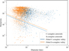 |
Fig. 1 Period–diameter distribution and fitted valley functions for S- and C-complex asteroid. |
3 Methods
3.1 Population selection
From the population of asteroids with recorded diameter, geometric visible albedo, and rotational period, we selected those belonging to the two main spectroscopic groups of the BusDeMeo taxonomy: the S-complex (S, Sa, Sq, Sr, and Sv classes) and the C-complex (B, C, Cb, Cg, Cgh, and Ch classes). We did not analyse X-complex asteroids because this spectral group encompasses multiple distinct compositions, and the limited number of objects with well-determined subclasses prevents a meaningful compositional separation.
We further restricted each taxonomic group using geometric visible albedo values, adopting a commonly used threshold of pV = 0.12 (Delbo et al. 2017) to separate low-albedo C-complex objects (pV ≤ 0.12) from higher-albedo S-complex objects (pv > 0.12) (Mainzer et al. 2011; Masiero et al. 2011; DeMeo & Carry 2013). We excluded objects whose best spectral classification was inconsistent with this albedo criteria (e.g. C-complex with pV greater than 0.12) to minimise contamination from ambiguous or uncertain classifications.
We also filtered the population to only include asteroids with a period quality value of at least 2− (2−, 2, 2+, 3−, 3) from the LCDB (Warner 2023). This selection process resulted in 6049 S-complex objects and 2947 C-complex objects, as shown in Fig. 1.
We also considered further filtering based on the YORP timescale of objects. Adopting a nominal YORP timescale of ~1 Myr for a 1 km body and the standard scaling τYORP ∝ D2 (Jewitt 2025), a Solar System age of 4.5 Gyr corresponds to D ≃ 65 km. Using the collisional lifetimes in the main belt from Marchi et al. (2006; based on Bottke et al. 2005), YORP evolution becomes comparable to or slower than catastrophic disruption timescales for D ≳ 50km. Removing such large objects from our sample has a negligible impact on the inferred valley slope because of their small number and limited statistical weight. We nevertheless retain D ≥ 50 km in our analysis for two reasons. First, they provide a useful comparison between the spin distributions of small, YORP-evolved asteroids and large bodies whose rotational states may remain essentially primordial. Second, the effective gigayear-scale YORP timescale remains uncertain, particularly due to stochastic reorientation by non-catastrophic collisions, so that the classical static estimate likely underestimates the long-term evolution time.
3.2 Quantifying the boundary of slow and fast rotators
To identify the valley between slow and fast rotators in both spectral complexes, we adopted the method of Zhou et al. (2025). This approach employs a semi-supervised machine-learning algorithm that classifies asteroids into two groups and determines the boundary line that separates them, which represents the centre of the valley. In their by manually defining an unclassified ‘grey zone’ as a reference region. The grey zone is centred on the presumed location of the valley, with its midpoint given by the reference line and its width corresponding to the distance along the y-axis from that line. Data points above this region were assigned to populations above the valley (spinners) and those below the valley (tumblers).
The reference line (i.e. the valley) and the associated grey zone were then iteratively updated by fitting the data using SVM to maximise the separation between the two subpopulations. In logarithmic coordinates, the valley is expressed as
![Mathematical equation: $\[\log~ P_{\mathrm{h}}=k ~\log~ D_{\mathrm{km}}+b,\]$](/articles/aa/full_html/2026/03/aa58305-25/aa58305-25-eq3.png) (1)
(1)
where the subscripts indicate the units. Through repeated updating of the grey zone and refitting, the model converges, and the reference line is identified as the functional form of the valley.
To account for uncertainties in asteroid diameters, we generated 1000 synthetic datasets for both the S- and C-complex populations, assigning each asteroid a diameter drawn from a Gaussian distribution centred on its measured value and with a standard deviation equal to its quoted uncertainty. In addition, to test the robustness of our results against the choice of the spectral score, we determined the values of k and b for different spectral score thresholds, ranging from one (the nominal value) to five. Increasing the spectral score restricts our dataset to higher quality data, while decreasing the number of data points (Appendix B).
4 Results and discussion
4.1 Distinct valley locations for S- and C-complex asteroids
Using data selected as described in Sects. 2 and 3.1, we first plotted the spin period histogram for S- and C-complex asteroids in the diameter range of 5–10 km (Fig. 2). We chose this size range because it contains sufficient data and falls in a regime where the YORP effect is effective (Rubincam 2000). Outside this range, the valley is expected to be absent or much less pronounced because smaller bodies are less well sampled, whereas larger ones experience weaker YORP torques.
The histogram in Fig. 2, which corresponds to the integrated valley region in the P–D diagram, shows clear local minima indicated by vertical arrows. These minima mostly occur at shorter spin periods for S-complex asteroids than for C-complex asteroids. The offset between the local minima for the two spectroscopic groups indicates that the valley of the S-complex population lies higher, i.e. towards shorter periods in the P–D plane, than the valley of the C-complex (Fig. 1).
To quantify this difference and its dependence on asteroid diameter, we applied the fitting method described in Sect. 3.2. The results are
![Mathematical equation: $\[P_s^*=11.6 \mathrm{~h}\left(\frac{D}{1 \mathrm{~km}}\right)^{0.718},\]$](/articles/aa/full_html/2026/03/aa58305-25/aa58305-25-eq4.png) (2)
(2)
for S-complex asteroids and
![Mathematical equation: $\[P_c^*=14.4 \mathrm{~h}\left(\frac{D}{1 \mathrm{~km}}\right)^{0.739},\]$](/articles/aa/full_html/2026/03/aa58305-25/aa58305-25-eq5.png) (3)
(3)
for C-complex asteroids, as shown in Fig. 1. Here, the symbols ![Mathematical equation: $\[P_{S / C}^{*}\]$](/articles/aa/full_html/2026/03/aa58305-25/aa58305-25-eq6.png) indicate the critical P-value as a function of D for each asteroid compositional complex, namely
indicate the critical P-value as a function of D for each asteroid compositional complex, namely ![Mathematical equation: $\[P_{S / C}^{*} \equiv P_{S / C}^{*}(D)\]$](/articles/aa/full_html/2026/03/aa58305-25/aa58305-25-eq7.png) . Because Eqs. (2) and (3), represent distinct functions, this provides the first clear, quantitative evidence that the location of the valley depends on spectral class. The functions
. Because Eqs. (2) and (3), represent distinct functions, this provides the first clear, quantitative evidence that the location of the valley depends on spectral class. The functions ![Mathematical equation: $\[P_{s}^{*}(D)\]$](/articles/aa/full_html/2026/03/aa58305-25/aa58305-25-eq8.png) and
and ![Mathematical equation: $\[P_{c}^{*}(D)\]$](/articles/aa/full_html/2026/03/aa58305-25/aa58305-25-eq9.png) describe both the position and the slope of the valley as functions of the asteroid size for each spectral complex.
describe both the position and the slope of the valley as functions of the asteroid size for each spectral complex.
For each complex, by dividing the rotation period of each asteroid, P, by the corresponding valley values, ![Mathematical equation: $\[P_{S / C}^{*}\]$](/articles/aa/full_html/2026/03/aa58305-25/aa58305-25-eq10.png) , we obtain the dimensionless ratio
, we obtain the dimensionless ratio ![Mathematical equation: $\[P / P_{S / C}^{*}\]$](/articles/aa/full_html/2026/03/aa58305-25/aa58305-25-eq11.png) , which measures the offset of an asteroid from the valley. Objects with
, which measures the offset of an asteroid from the valley. Objects with ![Mathematical equation: $\[P / P_{S / C}^{*}\]$](/articles/aa/full_html/2026/03/aa58305-25/aa58305-25-eq12.png) < 1 rotate faster than those at the centre of the valley, while those with
< 1 rotate faster than those at the centre of the valley, while those with ![Mathematical equation: $\[P / P_{S / C}^{*}\]$](/articles/aa/full_html/2026/03/aa58305-25/aa58305-25-eq13.png) > 1 rotate more slowly. In this representation, the valley appears as a deficit of objects near
> 1 rotate more slowly. In this representation, the valley appears as a deficit of objects near ![Mathematical equation: $\[P / P_{S / C}^{*}\]$](/articles/aa/full_html/2026/03/aa58305-25/aa58305-25-eq14.png) ≃ 1. Fig. 3 shows the distribution of the normalised rotational periods,
≃ 1. Fig. 3 shows the distribution of the normalised rotational periods, ![Mathematical equation: $\[P / P_{S / C}^{*}\]$](/articles/aa/full_html/2026/03/aa58305-25/aa58305-25-eq15.png) , for the S- and C complex asteroids across all diameter values. Both histograms clearly show the valley between fast and slow rotators, further supporting its presence.
, for the S- and C complex asteroids across all diameter values. Both histograms clearly show the valley between fast and slow rotators, further supporting its presence.
We conclude that in P − D space (Figure 1), the S-complex valley is higher than the C-complex valley. Although the fit suggests that the two complexes may differ in both offset and slope, applying the uncertainty estimation method described in Sect. 3.2 shows that the slope difference is not statistically significant given the current sample size and diameter uncertainties (Fig. 5). Thus, we cannot conclude whether the contrast between S- and C-complex asteroids also manifests as a slope difference. However, what is robust across all tests is that the S-complex valley lies above the C-complex valley. Fig. 4, shows resulting fitted valley functions, clearly demonstrating that the S-complex valleys generally lie above those of the C-complex. The figure also shows that the uncertainty is the smallest for D between ~10 and 20 km, due to the smaller uncertainties in relative diameter at these sizes. Fig. 5 shows the results of our method to estimate uncertainties in the valley parameters, k and b (Sect. 3) and the distinct distributions of these parameters (Eq. 1) for S- and C-complex asteroids. Larger values of b correspond to lower locations in the P–D diagram. The S-complex parameters lie below those of the C-complex, further demonstrating that the S-complex valley is systematically higher. Our method allows us to conclude that our results are robust against uncertainties in the observational data. In addition, we tested the robustness of our results as a function of the adopted threshold for the spectral score, which affects the selection of asteroids included in the study. Fig. B.1 shows the values of the valley parameters k and b when we apply our method with different spectral score thresholds. Because the results lie within the distribution of the k and b parameters when uncertainties in the data are considered, we conclude that our results are robust against selection imposed by the spectral score threshold.
Zhou et al. (2025) found that the valley correlates strongly with the separatrix between spinners and tumblers, corresponding to the location where collisional excitation and frictional damping are balanced. The timescale of collisional excitation for an asteroid of bulk density ρ can be estimated as
![Mathematical equation: $\[\tau_{\mathrm{col}} \sim 113 ~\mathrm{Myr}\left(\frac{D}{1 \mathrm{~km}}\right)^{(4 \alpha-10) / 3}\left(\frac{P}{8 \mathrm{~h}}\right)^{(1-\alpha) / 3}\left(\frac{\rho}{2 \mathrm{~g} \mathrm{~cm}^{-3}}\right)^{(\alpha-1) / 3},\]$](/articles/aa/full_html/2026/03/aa58305-25/aa58305-25-eq20.png) (4)
(4)
using the standard estimation of collisional probability for asteroids (see details in Farinella et al. 1998; Zhou et al. 2025). The dependence of Eq. (4) on bulk density was not explicitly shown by Zhou et al. (2025), as that work assumed equal densities for the impactor and the target asteroid. In this study, we adopt a mean bulk density of 2 g cm−3 for impactors, while the bulk densities of S- and C-complex asteroids are taken to be 3 and 1.5 g cm−3, respectively. Here, α is the power-index of the differential size-frequency distribution of asteroids, which determines the number of impactors.
The frictional damping timescale depends on the material parameter Q/k2. Tumbling causes the asteroid to undergo time-varying internal deformation as the orientation of its rotation axis continuously changes relative to its principal axes (e.g., Burns et al. 1973; Harris 1994; Pravec et al. 2014). The efficiency of this deformation is described by the degree-2 Love number k2, which quantifies the amplitude of the induced gravitational potential relative to the external forcing. A small k2 indicates that the body resists deformation and stores only a small amount of elastic strain energy. For a homogeneous elastic body, k2 is determined by the competition between self-gravity and internal rigidity. In the limit where rigidity dominates over self-gravity (μ ≫ ρgR), k2 can be expressed as
![Mathematical equation: $\[k_2 \sim \frac{\pi G \rho^2 D^2}{19 \mu},\]$](/articles/aa/full_html/2026/03/aa58305-25/aa58305-25-eq21.png) (5)
(5)
where μ is the shear modulus (rigidity) characterising the elastic resistance to shear deformation. This relation shows that small bodies (e.g. rubble-pile asteroids) possess extremely small k2 values due to both weak self-gravity and low effective rigidity. The stored strain energy is partially dissipated as heat through internal friction, quantified by the tidal quality factor Q. This parameter measures the ratio of elastic energy stored to that lost per cycle of deformation, with a lower Q indicating stronger dissipative processes. A high Q corresponds to weak dissipation (nearly elastic response), while a low Q indicates strong internal friction and rapid energy loss.
Therefore, a high Q/k2 or μQ corresponds to a longer damping timescale:
![Mathematical equation: $\[\tau_{\mathrm{damp}} \simeq A \frac{\mu Q}{2 \pi^3 \rho} P^3 D^{-2},\]$](/articles/aa/full_html/2026/03/aa58305-25/aa58305-25-eq22.png) (6)
(6)
where A ~ 18 is a dimensionless shape factor (Breiter et al. 2012; Pravec et al. 2014). Large μQ values correspond to weak energy loss and slow damping, whereas small μQ values produce rapid relaxation towards principal-axis rotation. Zhou et al. (2025) provide a normalised form:
![Mathematical equation: $\[\tau_{\text {damp }} \simeq 0.1 ~\mathrm{Myr}\left(\frac{\mu Q}{10^9 \mathrm{Pa}}\right)\left(\frac{\rho}{2 \mathrm{~g} \mathrm{~cm}^{-3}}\right)^{-1}\left(\frac{D}{1 \mathrm{~km}}\right)^{-2}\left(\frac{P}{8 \mathrm{~h}}\right)^3.\]$](/articles/aa/full_html/2026/03/aa58305-25/aa58305-25-eq23.png) (7)
(7)
Equating the excitation and damping timescales (Eqs. (4) and (7)), yield the condition at which these two processes are balanced:
![Mathematical equation: $\[\begin{aligned}P=~ & 8 \mathrm{~h} \cdot 283^{3 /(\alpha+8)}\left(\frac{\mu Q}{4 \times 10^9 \mathrm{~Pa}}\right)^{-3 /(8+\alpha)}\left(\frac{\rho}{2 \mathrm{~g} \mathrm{~cm}^{-3}}\right)^{(\alpha+2) /(\alpha+8)} \\& \cdot\left(\frac{D}{1 \mathrm{~km}}\right)^{(4 \alpha-4) /(8+\alpha)} \cdot\end{aligned}\]$](/articles/aa/full_html/2026/03/aa58305-25/aa58305-25-eq24.png) (8)
(8)
This defines the boundary of the distribution of tumblers. The centre of the valley, as detected using the machine-learning method, lies slightly above this boundary:
![Mathematical equation: $\[\begin{aligned}P^*=~ & 8 \mathrm{~h} \cdot 7^{3 /(\alpha+8)}\left(\frac{\mu Q}{4 \times 10^9 \mathrm{~Pa}}\right)^{-3 /(8+\alpha)}\left(\frac{\rho}{2 \mathrm{~g} \mathrm{~cm}^{-3}}\right)^{(\alpha+2) /(\alpha+8)} \\& \cdot\left(\frac{D}{1 \mathrm{~km}}\right)^{(4 \alpha-4) /(8+\alpha)}.\end{aligned}\]$](/articles/aa/full_html/2026/03/aa58305-25/aa58305-25-eq25.png) (9)
(9)
Zhou et al. (2025) found that, assuming α = 3.2, a global fit to all asteroids requires μQ of 4 × 10⁹ Pa, which is several orders of magnitude below monolithic values (1011–1013 Pa). Comparing Eqs. (2), (3) and (9), we find α ~ 3 for both S- and C-complex asteroids. Adopting ρ = 1.5 g cm−3 for C-complex asteroids and ρ = 3 g cm−3 for S-complex asteroids (Fienga et al. 2020), we obtain μQ ~ 1.3 × 10¹⁰ Pa for S-complex and μQ ~ 2 × 10⁹ Pa for C-complex asteroids. This is consistent with μQ ~ 4 × 10⁹ Pa for the full asteroid population reported by Zhou et al. (2025).
Following Breiter et al. (2012), we adopt a phenomenological Q-model in which the quality factor is treated as frequency-independent. Although more realistic rheological models may predict a frequency dependence of Q, such effects are poorly constrained for asteroid materials and are commonly neglected in analytical treatments of wobble damping. Importantly, our analysis focuses on the relative dissipation efficiencies between asteroid classes; therefore, any similar frequency dependence of Q across compositions would not affect our qualitative conclusions.
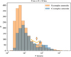 |
Fig. 2 Spin-period distribution of S-complex and C-complex asteroids in the 5–10 km diameter range. The local minimum in each distribution corresponds to the valley of the P-D diagram. The minimum for C-complex asteroids (blue) occurs at longer periods than for S-complex asteroids (orange). |
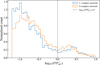 |
Fig. 3 Normalised distributions of the dimensionless offset from the fitted valley loci, |
![Mathematical equation: $\[\log _{10}\left(P / P_{S}^{*}\right)\]$](/articles/aa/full_html/2026/03/aa58305-25/aa58305-25-eq16.png)
![Mathematical equation: $\[\log _{10}\left(P / P_{C}^{*}\right)\]$](/articles/aa/full_html/2026/03/aa58305-25/aa58305-25-eq17.png)
![Mathematical equation: $\[\log _{10}\left(P / P_{S}^{*}\right)\]$](/articles/aa/full_html/2026/03/aa58305-25/aa58305-25-eq18.png)
![Mathematical equation: $\[\log _{10}\left(P / P_{C}^{*}\right)\]$](/articles/aa/full_html/2026/03/aa58305-25/aa58305-25-eq19.png)
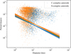 |
Fig. 4 Period–diameter (P − D) distribution for S-complex and C-complex asteroids. The lines show the fitted functions for the S- and C-complex valleys derived from the synthetic datasets generated according to the diameter uncertainties. |
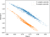 |
Fig. 5 Distributions of valley parameters k and b (Eq. (1)) for S- and C-complex asteroids, derived from fits to synthetic datasets that account for diameter uncertainties. Larger values of b correspond to a lower vertical position of the valley in the P–D diagram. |
4.2 Implications for internal structure and material properties
The offset between the S- and C-complex valleys provides evidence that the balance between collisional excitation and frictional damping differs for S- and C- complex asteroids through μQ. The slower transitional periods (lower valleys) of C-complex asteroids indicate stronger damping and therefore smaller μQ, consistent with higher porosity, weaker cohesion, and greater energy loss per cycle. In contrast, the higher valleys of S-complex asteroids imply more elastic, less dissipative interiors. These denser, silicate-dominated aggregates require faster spins to damp their tumbling motion (e.g. τdamp ∝ P3 in Eq. (6)) before their rotation is re-excited by collisions, whereas carbonaceous C-complex bodies deform more readily and dissipate rotational energy, allowing them to maintain principal-axis rotation at lower spin rates. Laboratory tensile-strength measurements of carbonaceous meteorites support this interpretation, showing strengths that are an order of magnitude lower than those of ordinary chondritic, silicate-rich analogues (Pohl & Britt 2020).
The parameter μQ also depends on near-surface structure. In the model of Nimmo & Matsuyama (2019), a thicker regolith layer leads to more energy dissipation and hence to a smaller μQ. Regolith is shaped by surface activity, such as space weathering and thermal fatigue (Delbo et al. 2014), as well as by internal processes including landslides, seismic shaking, and creep (e.g. Zhang et al. 2018; Brisset et al. 2018; Cheng et al. 2021). However, the ‘regolith’ implied in the Q/k2 framework of Nimmo & Matsuyama (2019) does not necessarily correspond to the near-surface regolith usually discussed in thermal models of small asteroids. In the Q/k2 formulation, the dissipative layer is the portion of the body that contributes to tidal energy dissipation, with a characteristic thickness that can reach tens of metres or more (Nimmo & Matsuyama 2019; Pou & Nimmo 2024). By contrast, in thermal contexts, regolith thickness is typically assumed to be of the order of a few thermal skin depths (i.e. a few centimetres), and S-type asteroids are expected to develop thicker near-surface regolith layers than C-complex asteroids (Cambioni et al. 2021).
Beyond rotation, μQ also governs the efficiency of tidal evolution in binary asteroids. Approximately 15% of asteroids are binaries (Pravec et al. 2006), whose long-term evolution is driven by tidal torques inversely proportional to μQ (e.g. Murray & Dermott 1999). A lower μQ for C-complex bodies implies stronger tidal dissipation and faster orbital evolution, potentially contributing to the observed deficit of C-complex binaries (Minker & Carry 2023; Liberato et al. 2024).
The physically significant quantity is the dimensionless ratio Q/k2, whose modelling remains uncertain. Equation (5) assumes an elastic sphere, which does not apply to rubble-pile asteroids. Therefore, the rigidity μ in Eq. (5) is not a true material modulus but an effective parameter. The mapping from Q/k2 to μQ, and ultimately to internal structure, is degenerate at the current stage. We briefly review other models of Q/k2 derived from Eq. (5) to illustrate how Q/k2 (or μQ) reflects the internal structure and material properties of rubble-pile asteroids.
Goldreich & Sari (2009) first derived k2 for a rubble pile by considering void-mediated yielding within a granular aggregate, finding
![Mathematical equation: $\[k_2 \sim \rho R ~\sqrt{\frac{G \epsilon_{\mathrm{Y}}}{\mu_{\mathrm{r}}}},\]$](/articles/aa/full_html/2026/03/aa58305-25/aa58305-25-eq26.png) (10)
(10)
where ϵY is the characteristic yield strain (~10−2) and μr is the effective rigidity of rubble piles. The damping timescale is therefore
![Mathematical equation: $\[\tau_{\text {damp }}=\frac{Q}{19 \pi^2} \sqrt{\frac{G \mu_{\mathrm{r}}}{\epsilon_{\mathrm{Y}}}} \frac{P^3}{D},\]$](/articles/aa/full_html/2026/03/aa58305-25/aa58305-25-eq27.png) (11)
(11)
which yields a valley function (combining Eqs. (4) and (11)):
![Mathematical equation: $\[P \propto\left(\sqrt{\mu_{\mathrm{r}}} Q\right)^{-3 /(8+\alpha)} D^{(4 \alpha-7) /(8+\alpha)}.\]$](/articles/aa/full_html/2026/03/aa58305-25/aa58305-25-eq28.png) (12)
(12)
This model predicts a valley slope k = (4α − 7)/(8 + α) ≃ 0.51, smaller than the observed range of 0.60–0.85 (Zhou et al. 2025, and Fig. 5), suggesting that additional size-dependent dissipation must be present.
The quality factor may also depend on size for rubble piles. Nimmo & Matsuyama (2019) developed a model in which energy loss only occurs within a surface regolith (a dissipative layer) of thickness h. The resulting effective quality factor scales inversely with the square of h, so that thinner, looser surface layers dissipate more efficiently. The approximate scaling of the quality factor Q is
![Mathematical equation: $\[Q \propto\left(\frac{D}{h}\right)^2.\]$](/articles/aa/full_html/2026/03/aa58305-25/aa58305-25-eq29.png) (13)
(13)
This indicates that for a given regolith thickness h, Q increases with diameter D. This trend arises because larger bodies experience smaller surface strain per unit stress. A rubble pile with a thick (tens-of-metres) regolith therefore exhibits a larger Q/k2 and, consequently, a larger effective μQ than a smaller object. The resulting Q/k2 ∝ D is consistent with the trend reported in (Jacobson & Scheeres 2011), which assumes that binary asteroids are in balance between tidal effect and the binary YORP effect. Pou & Nimmo (2024) used the ages of asteroid pairs to place quantitative bounds on Q/k2 for both primaries and secondaries in 13 binary systems. They constrained Q/k2 ranges from 104 to 106 for asteroid (3749) Balam with D ~ 2 km, with regolith height h estimated between 30 m and 100 m. Translating to the μQ prescription using Eq. (5), we obtain μQ ~ 107–109 Pa, far lower than values for monolithic bodies. These Q/k2 values remain uncertain because previous analyses neglected the recently proposed Binary Yarkovsky (BYarkovsky) effect (Zhou et al. 2024; Zhou 2024), an eclipse-driven thermal recoil capable of contracting binary orbits. Incorporating this additional torque will be essential for future self-consistent derivations of Q/k2 and μQ.
In summary, the upward displacement of the S-complex valley relative to the C-complex valley in the P–D diagram can be traced to a higher μQ, reflecting more rigid and less dissipative material behaviour. This compositional dependence links the rotational dynamics of single asteroids with the tidal and thermal evolution of binary systems, providing a unified diagnostic of internal structure and surface properties across the asteroid population.
This analysis provides observational evidence that asteroid spin-rate distributions are governed by a nuanced interplay between composition, internal structure, and evolutionary timescales. Accounting for these factors is essential for modelling spin evolution and assessing the mechanical response of near-Earth objects in planetary defence contexts.
Looking ahead, these results also have implications for planetary defence. The same physical processes shaping the spin-rate distributions of main-belt asteroids also operate in near-Earth objects (NEOs) and potentially hazardous objects (PHOs), where material properties and internal structure inform impact-risk assessments. Forthcoming surveys such as the Large Synoptic Survey Telescope (LSST), NASA’s NEO Surveyor, and potentially ESA’s Near-Earth Object Mission in the Infrared (NEOMIR) space telescopes, dramatically will increase the number of NEOs and PHOs with well-measured light curves. Extending the present analysis to smaller and potentially hazardous bodies will enable tighter constraints on their bulk strength and spin-dependent failure modes, which are central to evaluating mitigation strategies. Moreover, because the Yarkovsky effect is intrinsically linked to an asteroid’s rotation state, a refined understanding of spin evolution directly improves predictions of long-term orbital drift, enhancing our ability to model, track, and forecast the trajectories of objects that may pose a threat to Earth.
5 Conclusions
By combining MP3C data with the semi-supervised method of Zhou et al. (2025), we show that asteroid rotation distributions differ between the two major spectral complexes. Both populations display similar patterns, with a measurable deficit of objects at intermediate periods forming the valley in the period–diameter (P − D) diagram. Notably, the C-complex valley occurs at longer periods than the S-complex valley, reflecting intrinsic compositional and structural differences between the spectral classes. These results demonstrate that spectral information plays a pivotal role in interpreting asteroid rotational evolution, as some of these trends may be less apparent in wider population studies.
These results highlight the potential of MP3C as a relational database for population-level studies of asteroids, particularly regarding the evolutionary processes of small bodies. Future work could extend this analysis to individual subclasses within the complexes, or to rarer spectral types (V-, T-, and D-class asteroids). However, both approaches are limited by smaller sample sizes, which may require adapting current methods, developing alternative approaches, or collecting additional data. As the dataset expands with new observations from the LSST and Gaia data release 4, it will provide the leverage needed to perform these follow-up analyses and to test the robustness of our findings, thereby improving our understanding of the under-lying mechanisms responsible for the observed differences in rotational properties across asteroid populations.
Acknowledgements
This work is based on data provided by the Minor Planet Physical Properties Catalogue (MP3C; mp3c.oca.eu). T. J. Dyer acknowledges financial support from French Space Agency CNES and the Université Côte d’Azur (UniCA). W.-H. Zhou acknowledges support from the Japan Society for the Promotion of Science (JSPS) Fellowship (P25021). M. Delbo also acknowledges support from CNES. The work of J. Ďurech was supported by the grant 23-04946S of the Czech Science Foundation.
References
- Athanasopoulos, D., Hanuš, J., Avdellidou, C., et al. 2024, A&A, 690, A215 [NASA ADS] [CrossRef] [EDP Sciences] [Google Scholar]
- Avdellidou, C., Delbo, M., Morbidelli, A., et al. 2022, A&A, 665, L9 [NASA ADS] [CrossRef] [EDP Sciences] [Google Scholar]
- Barucci, M., Capria, M., Coradini, A., & Fulchignoni, M. 1987, Icarus, 72, 304 [NASA ADS] [CrossRef] [Google Scholar]
- Binzel, R. P. 1984, Icarus, 57, 294 [Google Scholar]
- Binzel, R. P., & Xu, S. 1993, Science, 260, 186 [NASA ADS] [CrossRef] [Google Scholar]
- Birlan, M., Fulchignoni, M., & Barucci, M. A. 1996, Icarus, 124, 352 [Google Scholar]
- Bottke, W. F., Durda, D. D., Nesvorný, D., et al. 2005, Icarus, 179, 63 [Google Scholar]
- Breiter, S., & Murawiecka, M. 2015, MNRAS, 449, 2489 [Google Scholar]
- Breiter, S., Rożek, A., & Vokrouhlický, D. 2011, MNRAS, 417, 2478 [Google Scholar]
- Breiter, S., Rożek, A., & Vokrouhlickỳ, D. 2012, MNRAS, 427, 755 [Google Scholar]
- Brisset, J., Colwell, J., Dove, A., et al. 2018, Progr. Earth Planet. Sci., 5, 73 [Google Scholar]
- Burns, J. A., Safronov, V., & Gold, T. 1973, MNRAS, 165, 403 [NASA ADS] [CrossRef] [Google Scholar]
- Bus, S. J., & Binzel, R. P. 2002, Icarus, 158, 106 [CrossRef] [Google Scholar]
- Cambioni, S., Delbo, M., Poggiali, G., et al. 2021, Nature, 598, 49 [NASA ADS] [CrossRef] [Google Scholar]
- Carbognani, A. 2011, Icarus, 211, 519 [Google Scholar]
- Carbognani, A. 2017, Planet. Space Sci., 147, 1 [Google Scholar]
- Carvano, J. M., Hasselmann, P. H., Lazzaro, D., & Mothé-Diniz, T. 2010, A&A, 510, A43 [NASA ADS] [CrossRef] [EDP Sciences] [Google Scholar]
- Cheng, B., Yu, Y., Asphaug, E., et al. 2021, Nat. Astron., 5, 134 [Google Scholar]
- Cicalò, S., & Scheeres, D. J. 2010, Celest. Mech. Dyn. Astron., 106, 301 [Google Scholar]
- Dahlgren, M., Lahulla, J., & Lagerkvist, C.-I. 1999, Icarus, 138, 259 [Google Scholar]
- Delbo, M., Libourel, G., Wilkerson, J., et al. 2014, Nature, 508, 233 [Google Scholar]
- Delbo, M., Walsh, K., Bolin, B., Avdellidou, C., & Morbidelli, A. 2017, Science, 357, 1026 [NASA ADS] [CrossRef] [Google Scholar]
- Delbo, M., Avdellidou, C., Bruot, N., & Erard, S. 2022, in European Planetary Science Congress, EPSC2022-323 [Google Scholar]
- DeMeo, F., & Carry, B. 2013, Icarus, 226, 723 [NASA ADS] [CrossRef] [Google Scholar]
- DeMeo, F. E., Binzel, R. P., Slivan, S. M., & Bus, S. J. 2009, Icarus, 202, 160 [Google Scholar]
- Ďurech, J., & Hanuš, J. 2023, A&A, 675, A24 [NASA ADS] [CrossRef] [EDP Sciences] [Google Scholar]
- Erasmus, N., Kramer, D., McNeill, A., et al. 2021, MNRAS, 506, 3872 [NASA ADS] [CrossRef] [Google Scholar]
- Farinella, P., Vokrouhlickỳ, D., & Hartmann, W. K. 1998, Icarus, 132, 378 [NASA ADS] [CrossRef] [Google Scholar]
- Fienga, A., Avdellidou, C., & Hanuš, J. 2020, MNRAS, 492, 589 [Google Scholar]
- Fornasier, S., Clark, B., & Dotto, E. 2011, Icarus, 214, 131 [NASA ADS] [CrossRef] [Google Scholar]
- Goldreich, P., & Sari, R. 2009, ApJ, 691, 54 [NASA ADS] [CrossRef] [Google Scholar]
- Harris, A. W. 1994, Icarus, 107, 209 [NASA ADS] [CrossRef] [Google Scholar]
- Harris, A. W., & Burns, J. A. 1979, Icarus, 40, 115 [Google Scholar]
- Howell, E. S., Merényi, E., & Lebofsky, L. A. 1994, J. Geophys. Res.: Planets, 99, 10847 [Google Scholar]
- Jacobson, S. A., & Scheeres, D. J. 2011, ApJ, 736, L19 [NASA ADS] [CrossRef] [Google Scholar]
- Jewitt, D. 2025, Planet. Sci. J., 6, 12 [Google Scholar]
- Jewitt, D. C., & Luu, J. X. 1990, AJ, 100, 933 [NASA ADS] [CrossRef] [Google Scholar]
- Liberato, L., Tanga, P., Mary, D., et al. 2024, A&A, 688, A50 [NASA ADS] [CrossRef] [EDP Sciences] [Google Scholar]
- Mahlke, M., Carry, B., & Mattei, P.-A. 2022, A&A, 665, A26 [NASA ADS] [CrossRef] [EDP Sciences] [Google Scholar]
- Mainzer, A., Grav, T., Bauer, J., et al. 2011, ApJ, 743, 156 [NASA ADS] [CrossRef] [Google Scholar]
- Mansour, J.-A., Popescu, M., de León, J., & Licandro, J. 2019, MNRAS, 491, 5966 [Google Scholar]
- Marchi, S., Paolicchi, P., Lazzarin, M., & Magrin, S. 2006, AJ, 131, 1138 [NASA ADS] [CrossRef] [Google Scholar]
- Masiero, J. R., Mainzer, A. K., Grav, T., et al. 2011, ApJ, 741, 68 [Google Scholar]
- Minker, K., & Carry, B. 2023, A&A, 672, A48 [NASA ADS] [CrossRef] [EDP Sciences] [Google Scholar]
- Murray, C. D., & Dermott, S. F. 1999, Solar System Dynamics (Cambridge University Press) [Google Scholar]
- Nimmo, F., & Matsuyama, I. 2019, Icarus, 321, 715 [NASA ADS] [CrossRef] [Google Scholar]
- Pohl, L., & Britt, D. T. 2020, Meteor. Planet. Sci., 55, 962 [Google Scholar]
- Pou, L., & Nimmo, F. 2024, Icarus, 411, 115919 [NASA ADS] [CrossRef] [Google Scholar]
- Pravec, P., & Harris, A. W. 2000, Icarus, 148, 12 [NASA ADS] [CrossRef] [Google Scholar]
- Pravec, P., Scheirich, P., Kusnirak, P., et al. 2006, Icarus, 181, 63 [NASA ADS] [CrossRef] [Google Scholar]
- Pravec, P., Harris, A., Vokrouhlický, D., et al. 2008, Icarus, 197, 497 [NASA ADS] [CrossRef] [Google Scholar]
- Pravec, P., Scheirich, P., Ďurech, J., et al. 2014, Icarus, 233, 48 [NASA ADS] [CrossRef] [Google Scholar]
- Pravec, P., Fatka, P., Vokrouhlický, D., et al. 2018, Icarus, 304, 110 [Google Scholar]
- Rubincam, D. P. 2000, Icarus, 148, 2 [Google Scholar]
- Tedesco, E. F., & Gradie, J. 1987, AJ, 93, 738 [Google Scholar]
- Tholen, D. J. 1984, PhD Thesis, The University of Arizona [Google Scholar]
- Vavilov, D., & Carry, B. 2025, A&A, 693, A66 [NASA ADS] [CrossRef] [EDP Sciences] [Google Scholar]
- Vokrouhlický, D., Breiter, S., Nesvorný, D., & Bottke, W. 2007, Icarus, 191, 636 [Google Scholar]
- Walsh, K. J., Richardson, D. C., & Michel, P. 2008, Nature, 454, 188 [Google Scholar]
- Warner, B. 2023, Asteroid Lightcurve Data Base (LCDB) Technical Documentation [Google Scholar]
- Warner, B. D., Harris, A. W., & Pravec, P. 2009, Icarus, 202, 134 [NASA ADS] [CrossRef] [Google Scholar]
- Zhang, Y., Richardson, D. C., Barnouin, O. S., et al. 2018, ApJ, 857, 15 [Google Scholar]
- Zhou, W.-H. 2024, A&A, 692, L2 [NASA ADS] [CrossRef] [EDP Sciences] [Google Scholar]
- Zhou, W.-H., Vokrouhlickỳ, D., Kanamaru, M., et al. 2024, ApJ, 968, L3 [NASA ADS] [CrossRef] [Google Scholar]
- Zhou, W.-H., Michel, P., Delbo, M., et al. 2025, Nat. Astron., 9, 493 [Google Scholar]
Appendix A References to taxonomic schemes
Taxonomic schemes used in MP3C:
Barucci: (Barucci et al. 1987)
Binzel: (Binzel & Xu 1993)
Birlan: (Birlan et al. 1996)
Bus: (Bus & Binzel 2002)
Bus-DeMeo: (DeMeo et al. 2009)
Carvano: (Carvano et al. 2010)
Dahlgren-Lagerkvist: (Dahlgren et al. 1999)
DeMeo-Carry: (DeMeo & Carry 2013)
Fornasier: (Fornasier et al. 2011)
Gradie-Tedesco: (Tedesco & Gradie 1987)
Howell: (Howell et al. 1994)
Jewitt-Luu: (Jewitt & Luu 1990)
Mahlke: (Mahlke et al. 2022)
Popescu: (Mansour et al. 2019)
Tholen: (Tholen 1984)
Appendix B Spectral score robustness
The spectral classification adopted in this work relies on a scoring-based aggregation of different taxonomic measurements, which necessarily involves a trade-off between sample size and classification reliability. To verify that our main results are not driven by the particular choice of spectral-score threshold used to define the working sample, we explicitly test the robustness of the fitted valley parameters to progressively stricter spectral-quality cuts. This appendix illustrates how the fitted valley solutions for the S-complex and C-complex populations evolve as the minimum spectral score requirement is increased.
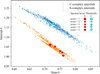 |
Fig. B.1 Same as Fig. 5, showing the distributions of the valley parameters k and b (Eq. 1) for S-complex and C-complex asteroids. Over-plotted points indicate the best-fit valley solutions obtained from the dataset using progressively stricter spectral-classification score thresholds between 1 and 5 (as indicated by different symbols). Because the symbols lie within the distributions from the nominal datasets (see text), this illustrates the robustness of the fitted parameters versus changes in the spectral score threshold to the adopted spectral-quality cut. |
All Tables
Weights assigned to different combinations of wavelengths and data collection methods.
All Figures
|
Fig. 1 Period–diameter distribution and fitted valley functions for S- and C-complex asteroid. |
| In the text | |
|
Fig. 2 Spin-period distribution of S-complex and C-complex asteroids in the 5–10 km diameter range. The local minimum in each distribution corresponds to the valley of the P-D diagram. The minimum for C-complex asteroids (blue) occurs at longer periods than for S-complex asteroids (orange). |
| In the text | |
|
Fig. 3 Normalised distributions of the dimensionless offset from the fitted valley loci, |
| In the text | |
|
Fig. 4 Period–diameter (P − D) distribution for S-complex and C-complex asteroids. The lines show the fitted functions for the S- and C-complex valleys derived from the synthetic datasets generated according to the diameter uncertainties. |
| In the text | |
|
Fig. 5 Distributions of valley parameters k and b (Eq. (1)) for S- and C-complex asteroids, derived from fits to synthetic datasets that account for diameter uncertainties. Larger values of b correspond to a lower vertical position of the valley in the P–D diagram. |
| In the text | |
|
Fig. B.1 Same as Fig. 5, showing the distributions of the valley parameters k and b (Eq. 1) for S-complex and C-complex asteroids. Over-plotted points indicate the best-fit valley solutions obtained from the dataset using progressively stricter spectral-classification score thresholds between 1 and 5 (as indicated by different symbols). Because the symbols lie within the distributions from the nominal datasets (see text), this illustrates the robustness of the fitted parameters versus changes in the spectral score threshold to the adopted spectral-quality cut. |
| In the text | |
Current usage metrics show cumulative count of Article Views (full-text article views including HTML views, PDF and ePub downloads, according to the available data) and Abstracts Views on Vision4Press platform.
Data correspond to usage on the plateform after 2015. The current usage metrics is available 48-96 hours after online publication and is updated daily on week days.
Initial download of the metrics may take a while.