| Issue |
A&A
Volume 707, March 2026
|
|
|---|---|---|
| Article Number | L17 | |
| Number of page(s) | 4 | |
| Section | Letters to the Editor | |
| DOI | https://doi.org/10.1051/0004-6361/202558326 | |
| Published online | 17 March 2026 | |
Letter to the Editor
Radio detection of a local little red dot
1
Instituto de Radioastronomía y Astrofísica, Universidad Nacional Autónoma de México, Apdo. Postal 3-72 Morelia, Michoacán 58089, Mexico
2
Instituto de Astronomía y Física del Espacio (IAFE) CONICET-Universidad de Buenos Aires, C1428 Buenos Aires, Argentina
★ Corresponding author: This email address is being protected from spambots. You need JavaScript enabled to view it.
Received:
30
November
2025
Accepted:
2
February
2026
Abstract
Context. One of the most important discoveries by the James Webb Space Telescope (JWST) is the unexpected existence of very large quantities of so-called little red dots (LRDs) in the early Universe (z > 4). These are compact luminous red galaxies with intriguing physical properties, one of which is the absence of radio detections.
Aims. We wish to know if LRDs give off radio emission produced by accreting intermediate-mass or supermassive black holes (IMBHs or SMBHs) or by frequent supernovae from a cluster of massive stars.
Methods. Assuming that LRDs at high redshifts have not been detected at radio wavelengths because they reside at large distances and/or the observational capabilities are limited, we present images made from archive Very Large Array (VLA) radio observations of J1047+0739 and J1025+1402. These are two analog candidate LRDs in the Local Universe at redshifts z = 0.1−0.2.
Results. The source J1047+0739 at z = 0.1682 is detected at 6.0 GHz in 2018 with the VLA-A as a compact source with a radius smaller than 0.2 arcsec (< 700 pc at d ≃ 750 Mpc). Its flux density was 117 ± 8 μJy and its in-band spectral index was −0.85 ± 0.24, which is typical of optically thin synchrotron emission. It was also detected at 5.0 GHz in 2010 with the VLA-C, showing a flux density of 130 ± 9 μJy. We also detect a compact source very near J1025+1402 (≃2″) with a flux density of 45 ± 10 μJy that might be tracing a kiloparsec-scale jet emanating from an IMBH or SMBH.
Conclusions. The observed flux densities can be provided by either a radio luminous supernova or an accreting IMBH or SMBH. However, the lack of significant variation in the flux density over eight years favors the IMBH–SMBH hypothesis. Radio time monitoring of this and other Local Little Red Dots (LLRDs) might help us solve the mystery of the radio silence of its cosmological counterparts.
Key words: supernovae: general / galaxies: jets / galaxies: nuclei
© The Authors 2026
 Open Access article, published by EDP Sciences, under the terms of the Creative Commons Attribution License (https://creativecommons.org/licenses/by/4.0), which permits unrestricted use, distribution, and reproduction in any medium, provided the original work is properly cited.
This article is published in open access under the Subscribe to Open model. This email address is being protected from spambots. You need JavaScript enabled to view it. to support open access publication.
1. Introduction
Abundant populations of little red dots (LRDs) at z > 4 have been unexpectedly discovered in several James Webb Space Telescope (JWST) surveys in the past few years (e.g. Matthee et al. 2024; Kocevski et al. 2025a; Labbe et al. 2025; Akins et al. 2025). LRDs are mostly observed between redshifts of z = 4 and z = 8 with a maximum peak density at z = 5 and an exponential decline in numbers at redshifts z < 4 (e.g. Billand et al. 2026). This implies that local little red dot (LLRD) candidates are scarce in the Local Universe.
The LRDs in the early Universe are extremely compact sources with average effective radii smaller than a few hundred parsecs, broad emission line widths of up to 2000 km s−1, and V-shaped spectral energy distributions. They are intrinsically red rather than dust-reddened (e.g. Guia et al. 2024; Schindler et al. 2025). These properties together were uncommon in known galaxies before the advent of JWST. LRDs are not detected or are very dim soft X-ray-emitters of less than 10 keV, and they have not been detected at radio wavelengths. These physical properties are puzzling, and to explain the dominant energy source of the high luminosities, two basic types of models have been proposed, one based on highly accreting intermediate-mass or supermassive black holes (IMBHs or SMBHs), and the other based on rich clusters of very massive stars. The latter have been challenged because of the extreme stellar masses that would be required to produce the high luminosity of LRDs in volumes with radii of only a few hundred parsecs (Pacucci et al. 2023). On the other hand, the absence of soft X-ray detections in LRDs challenged models of accreting IMBHs or SMBHs. However, this absence of X-rays can be explained by cold gas absorption in an IMBH or SMBH atmosphere with gas densities nH > 109 cm−3, column densities NH > 1024 cm−2 (e.g. Rusakov et al. 2026), and gas turbulent velocities of ∼500 km s−1 (e.g. Killi et al. 2024; Maiolino et al. 2025; Kocevski et al. 2025b). Other models attempted to explain the absence of X-rays and radio emission by invoking dust or free-free absorption, synchrotron self-absorption, and the disruption of magnetic field and X-ray coronae by super-Eddington accretion (Mazzolari et al. 2026; de Graaff et al. 2025).
In contrast to soft X-rays, radio jet emission may not be totally or even partially absorbed by neutral column densities of NH > 1024 cm−2. Radio jets are observed from mass-accreting stellar black holes (BHs), while soft X-rays are completely obscured (Rodríguez & Mirabel 2025 and references therein). However, LRDs in the early Universe so far have been radio-silent for unknown reasons (e.g. Mazzolari et al. 2026; Perger et al. 2025; Akins et al. 2025; Latif et al. 2025). The active galactic nucleus candidate PRIMER-COS 3866 at z = 4.66 was detected in the radio survey by Gloudemans et al. (2025). However, these authors noted that it lacks detectable Hα emission in its JWST spectrum and cannot be considered an LRD. In this context, the study of LRD analogs might help us understand why LRDs at high redshifts are radio-silent, and it might eventually lead to strategies that could result in their radio detection. An immediate way to test the different LRD models directly is analyzing archived radio observations of LLRD candidates.
The sources SDSS J1025+1402 (z = 0.10067) and SDSS J1047+0739 (z = 0.16828) were serendipitously identified for the first time in the Sloan Digital Sky Survey (SDSS) by Izotov & Thuan (2008) as metal-poor dwarf emission-line galaxies. The authors found signals of an intermediate-mass active galactic nucleus in these galaxies. The properties of these sources are given in Table 1 of Izotov & Thuan (2008). It was found that these compact dwarf galaxies had extraordinarily velocity-broadened Hα emission with luminosities ranging from 3 × 1041 to 2 × 1042 erg s−1. Their metallicity is very low, and their extraordinarily high broad Hα luminosities remained constant over periods of 3−7 yr, which probably rule out Type IIn supernovae (SNe) as a mechanism for the emission with broad velocities. More recently, Lin et al. (2026) showed that the properties of these two sources are fully consistent with those of high-redshift LRDs and that they might be local analogs.
We investigated whether the radio emission of LLRD analogs originates from a SN mechanism or from IMBH–SMBH accretion, and we estimated the expected level of LRD radio flux densities at high redshifts. The cosmological parameters employed in our study were obtained using the Javascript calculator from Wright (2006) and assuming a flat Planck Λ cold dark matter cosmology with H0 = 67.4 km s−1 Mpc−1, ΩM = 0.315, and ΩΛ = 0.685 (Planck Collaboration VI 2020).
In Sect. 2 the observations and data reduction are described. In Sect. 3 the results are presented, and in Sect. 4 we discuss them. Finally, in Sect. 5 we summarize our results and present our conclusions.
2. Observations and data reduction
Previous studies of these regions failed to detect radio continuum emission (Burke et al. 2021). We searched for observations of these two LLRDs in the US National Radio Astronomy Observatory (NRAO) archive. We found data in two Very Large Array (VLA) projects: 10B-156 (PI: C. Henkel) and 18A-413 (PI: F. Bauer). Both projects were observed in the VLA standard continuum mode (NRAO 2025).
In project 10B-156, both sources were observed. The array was in its C configuration. J1047+0739 was observed at epoch 2010 November 06 and J1025+1402 was observed at epoch 2010 October 25. In both epochs, 0521+166 = 3C138 was the amplitude calibrator. The gain calibrators were J1007+1356 for J1025+1402 and J1058+0133 for J1047+0739. The bootstrapped flux densities of J1007+1356 and J1058+0133 were 0.763 ± 0.002 and 3.010 ± 0.003 Jy, respectively. Each target was observed for an on-source integration time of 88 minutes.
The data of project 18A-413 were taken with the array in its highest angular resolution A configuration. Only J1047+0739 was observed at epoch 2018 April 20 for an on-source integration time of 19 minutes. The amplitude calibrator was 1331+305 = 3C286 and the gain calibrator was J1058+0133, with a bootstrapped flux density of 6.379 ± 0.024 Jy.
The data were analyzed in the standard manner using the Common Astronomy Software Applications (CASA; McMullin et al. 2007) package of NRAO and the pipeline provided for VLA observations. The data were calibrated using the NRAO VLA CASA pipeline1.
We made images using a robust weighting (Briggs 1995) of 0 to optimize the compromise between angular resolution and sensitivity. All images were also corrected for the primary beam response. The position, flux density, and angular dimensions of the sources were determined using the CASA task imfit, fitting the source in the image plane with a Gaussian ellipsoid function. In this task, the parameter uncertainties are estimated using a noise-weighted least-squares fit, with errors derived from the covariance matrix of the fit (Condon 1997).
3. Results
3.1. LLRD J1047+0739
The LLRD J1047+0739 was clearly detected at both epochs (2010 November 6 and 2018 April 20; see Fig. 1). The flux densities and other parameters of the observations of this source are listed in Table 1. At the second epoch (2018 April 20), the data were taken with the broadband correlator (with a total bandwidth of 4.0 GHz), and an in-band spectral index determination was possible. To do this, we divided the spectral windows into four 1 GHz wide sub-bands and determined the flux densities shown in Fig. 2. A least-squares fit to these flux densities gives
![Mathematical equation: $$ \begin{aligned} \log [{S\!}_{\nu }(\upmu \mathrm{Jy})] = (2.74 \pm 0.18) -(0.85 \pm 0.24)\,\log [\nu (\mathrm{GHz})]. \end{aligned} $$](/articles/aa/full_html/2026/03/aa58326-25/aa58326-25-eq1.gif) (1)
(1)
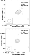 |
Fig. 1. Top: VLA contour image of the J1047+0739 region from project 10B-156. The contours start at ±3σ and increase by factors of |


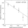 |
Fig. 2. Flux density as a function of frequency for J1047+0739 from the data of project 18A-413. The least-squares fit is indicated with a dashed line. |
VLA sources associated with J1025+1402 and J1047+0739.
3.2. LLRD J1025+1402
On the other hand, no radio source was found to coincide with the optical position of J1025+1402 in the 2010 October 25 observations that were made as part of project 10B-156. However, about 2″ east of it lies a radio source that is detected at the 4σ level with a flux density of 45 ± 10 μJy (Fig. 3). The properties of this source are listed in Table 1. The offset of 2″ is very reliable because the typical uncertainty in the position for observations of the VLA in configuration A at 6 GHz is about  (NRAO 2025). This means that the offset is significant at the 40σ level. According to the formulation of Anglada et al. (1998), the a priori probability of detecting a source with this flux density at the frequency of 5.0 GHz in a solid angle of 4 × 4 arcsec2 is only 0.0005, so the association of the radio source with J1025+1402 seems to be significant. We adopted a 4σ detection threshold for our targeted search because the solid angle we considered is small. A 4σ threshold has a false probability of 6.4 × 10⁻⁵ per resolution element. For a Nyquist sampling, the solid angle we considered has nine resolution elements. The probability of a false detection is thus only 0.0006.
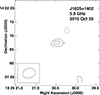 |
Fig. 3. VLA contour image of the J1025+1402 region from project 10B-156. The contours start at ±3σ and increase by factors of |


We estimated the upper limit to the angular size of the source following Lobanov (2005), and we found that the radio source is unresolved at a scale of  (< 4200 pc at d ≃ 450 Mpc). Future observations in VLA-A and VLA-B configurations may determine whether this extended radio emission is a kiloparsec-scale jet emanating from an IMBH or a SMBH. No additional analysis can be performed on J1025+1402 because the signal-to-noise ratio of the source detection is too low.
4. Discussion
4.1. The nature of the radio emission of LLRD J1047+0739
The spectral index of −0.85 found in J1047+0739 is typical of optically thin synchrotron emission and favors a nonthermal mechanism to produce the radio emission (Rodriguez et al. 1993) and possibly energize the LLRDs. The radio source is unresolved at a scale of  (< 250 pc at d ≃ 750 Mpc).
Another important result is the lack of significant flux density variability in the radio emission. By correcting the 5.0 GHz flux density of 2010 by a factor (5.0/6.0)−0.85 to compare with the 2018 flux density at 6.0 GHz, we found that the flux density has remained approximately constant over this 7.5 yr time period. This lack of variability in the radio flux density is consistent with the lack of variability in the r band reported for J1047+0739 at the 3−4% level by Burke et al. (2025) over a rest-frame baseline of ∼15 yr. Based on these properties, the radio emission from J1047+0739 might originate from either frequent SNe from a cluster of massive stars or from accretion onto an IMBH or SMBH in the system.
4.2. Supernova origin
The most radio-luminous SNe reach values of LR ∼ 1039 erg s−1 (Kulkarni et al. 1998; Waxman & Loeb 1999; Yao et al. 2022). The radio luminosity associated with LLRD J1047+0739 between rest frequencies ν2 and ν1 was calculated using the following equation:
 (2)
(2)
The radio luminosity was estimated by assuming that the power-law spectrum, Sν ∝ να, is valid between 1 and 10 GHz. In this frequency range, optically thin synchrotron emission dominates, and the spectral curvature is minimal (e.g. Condon 1992). The observed flux density is Sν = 117 μJy at ν = 6.0 GHz. For z = 0.16828, DL = 839 Mpc, and α = −0.85, we obtained SL = 1.5 × 1039 erg s−1. This value is comparable to that of the most luminous radio SNe known. We thus conclude that the radio emission observed from LLRD J1047+0739 can in principle be explained in terms of a luminous SN.
However, the lack of significant variability between 2010 and 2018 is an argument against an individual SN mechanism. The radio emission might be produced by the combined effect of past generations of SN explosions that injected relativistic electrons into the medium.
4.3. IMBH or SMBH origin
The radio luminosity of J1047+0739 is similar to that of Seyfert galaxies, in that the two types have similar radio luminosity functions. From a sample of 47 Seyfert galaxies (Rush et al. 1996), we found that the logarithmic mean and dispersion of the sample are given by log(LR) = 1038.2 ± 0.8 erg s−1. The radio luminosity of J1047+0739 falls at the high end of this range of values. We conclude that an IMBH or SMBH of moderate activity can explain the observed radio luminosity of J1047+0739.
4.4. Expected radio flux density at cosmological distances
The measured flux density of LLRD J1047+0739 can be used to predict the flux density expected for an identical source located at cosmological distances. For a radio source with a power-law spectrum given by Sν ∝ να, the flux density measured at the same frequency and different z values is given by
![Mathematical equation: $$ \begin{aligned} \left[{{{S\!}_{\nu }(z_1)} \over {{S\!}_{\nu }(z_0)}}\right] = \left[{{1 + z_0} \over {1 + z_1}}\right]^{-(\alpha +1)} \; \left[{{D_{\rm L} (z_0)} \over {D_{\rm L} (z_1)}}\right]^2, \end{aligned} $$](/articles/aa/full_html/2026/03/aa58326-25/aa58326-25-eq12.gif) (3)
(3)
where z is the redshift, Sν is the flux density, and DL is the luminosity distance. In our case, the reference is LLRD J1047+0739, for which z0 = 0.16828, DL = 839 Mpc, and α = −0.85.
The flux density for a source located in the region in which the number density of LRDs peaks, that is, z = 5 (DL = 47660 Mpc), is estimated as
 (4)
(4)
that is, the expected flux densities in the centimeter range are about 50 nJy. These low flux densities are only detectable with extremely long integrations, even by the next generation of radio interferometers. With next-generation VLA (ngVLA) band 2 (3.5−12.3 GHz) observations, a 100 h on-source integration time would be necessary to reach the thermal sensitivity (∼14 nJy; Rosero et al. 2021) required to detect the radio emission of cosmological LRDs with similar radio luminosity to that of LLRD J1047+0739.
5. Summary and conclusions
We have presented the analysis of archive VLA observations with the purpose of detecting radio continuum emission in LLRDs that might help us understand the radio silence of cosmological LRDs. We detected a source near J1025+1402 that might be tracing a kiloparsec-scale jet emanating from an IMBH or a SMBH. We also detected radio emission from the LLRD J1047+0739 in two epochs. Based on the in-band spectrum, the nature of the emission is optically thin synchrotron. The lack of significant flux density variability (≥20%) between the two epochs (2010 and 2018) suggests that the radio emission can be understood in terms of a BH with a nature similar to those of the BHs found in Seyfert galaxies or by the emission produced by previous generations of SNe. If the radio emission from cosmological LRDs is similar in luminosity to that produced by the LLRD J1047+0739, they will be detectable with long integrations with the next generation of centimeter interferometers.
Acknowledgments
The National Radio Astronomy Observatory is a facility of the National Science Foundation operated under cooperative agreement by Associated Universities, Inc. We thank an anonymous referee for valuable comments. LFR acknowledges support from grant CBF-2025-I-2471 of SECIHTI, Mexico.
References
- Akins, H. B., Casey, C. M., Lambrides, E., et al. 2025, ApJ, 991, 37 [Google Scholar]
- Anglada, G., Villuendas, E., Estalella, R., et al. 1998, AJ, 116, 2953 [Google Scholar]
- Billand, J.-B., Elbaz, D., Gentile, F., et al. 2026, A&A, 706, A29 [NASA ADS] [CrossRef] [EDP Sciences] [Google Scholar]
- Briggs, D. S. 1995, Ph.D. Thesis, New Mexico Institute of Mining and Technology [Google Scholar]
- Burke, C. J., Liu, X., Chen, Y.-C., et al. 2021, MNRAS, 504, 543 [NASA ADS] [CrossRef] [Google Scholar]
- Burke, C. J., Stone, Z., Shen, Y., et al. 2025, ArXiv e-prints [arXiv:2511.16082] [Google Scholar]
- Condon, J. J. 1992, ARA&A, 30, 575 [Google Scholar]
- Condon, J. J. 1997, PASP, 109, 166 [NASA ADS] [CrossRef] [Google Scholar]
- de Graaff, A., Rix, H.-W., Naidu, R. P., et al. 2025, A&A, 701, A168 [NASA ADS] [CrossRef] [EDP Sciences] [Google Scholar]
- Gaia Collaboration 2020, VizieR Online Data Catalog: I/350 [Google Scholar]
- Gloudemans, A. J., Duncan, K. J., Eilers, A.-C., et al. 2025, ApJ, 986, 130 [Google Scholar]
- Guia, C. A., Pacucci, F., & Kocevski, D. D. 2024, Res. Notes Am. Astron. Soc., 8, 207 [Google Scholar]
- Izotov, Y. I., & Thuan, T. X. 2008, ApJ, 687, 133 [Google Scholar]
- Killi, M., Watson, D., Brammer, G., et al. 2024, A&A, 691, A52 [NASA ADS] [CrossRef] [EDP Sciences] [Google Scholar]
- Kocevski, D. D., Finkelstein, S. L., Barro, G., et al. 2025a, ApJ, 986, 126 [Google Scholar]
- Kocevski, D., Finkelstein, S., Taylor, A., et al. 2025b, A&AS, 245, 139.07 [Google Scholar]
- Kulkarni, S. R., Frail, D. A., Wieringa, M. H., et al. 1998, Nature, 395, 663 [NASA ADS] [CrossRef] [Google Scholar]
- Labbe, I., Greene, J. E., Bezanson, R., et al. 2025, ApJ, 978, 92 [NASA ADS] [CrossRef] [Google Scholar]
- Latif, M. A., Aftab, A., Whalen, D. J., et al. 2025, A&A, 694, L14 [NASA ADS] [CrossRef] [EDP Sciences] [Google Scholar]
- Lin, X., Fan, X., Cai, Z., et al. 2026, ApJ, 997, 364 [Google Scholar]
- Lobanov, A. P. 2005, ArXiv e-prints [arXiv:astro-ph/0503225] [Google Scholar]
- Maiolino, R., Risaliti, G., Signorini, M., et al. 2025, MNRAS, 538, 1921 [Google Scholar]
- Matthee, J., Naidu, R. P., Brammer, G., et al. 2024, ApJ, 963, 129 [NASA ADS] [CrossRef] [Google Scholar]
- Mazzolari, G., Gilli, R., Maiolino, R., et al. 2026, A&A, 706, A372 [NASA ADS] [CrossRef] [EDP Sciences] [Google Scholar]
- McMullin, J. P., Waters, B., Schiebel, D., et al. 2007, Astronomical Data Analysis Software and Systems XVI, 376, 127 [NASA ADS] [Google Scholar]
- NRAO 2025, VLA Observational Status Summary, https://science.nrao.edu/facilities/vla/docs/manuals/oss [Google Scholar]
- Pacucci, F., Nguyen, B., Carniani, S., et al. 2023, ApJ, 957, L3 [CrossRef] [Google Scholar]
- Perger, K., Fogasy, J., Frey, S., et al. 2025, A&A, 693, L2 [NASA ADS] [CrossRef] [EDP Sciences] [Google Scholar]
- Planck Collaboration VI. 2020, A&A, 641, A6 [NASA ADS] [CrossRef] [EDP Sciences] [Google Scholar]
- Rodríguez, L. F., & Mirabel, I. F. 2025, ApJ, 986, 108 [Google Scholar]
- Rodriguez, L. F., Marti, J., Canto, J., et al. 1993, Rev. Mexicana Astron. Astrofis., 25, 23 [Google Scholar]
- Rosero, V., Carilli, C., Mason, B., et al. 2021, The 36th Annual New Mexico Symposium, 22 [Google Scholar]
- Rusakov, V., Watson, D., Nikopoulos, G. P., et al. 2026, Nature, 649, 574 [Google Scholar]
- Rush, B., Malkan, M. A., & Edelson, R. A. 1996, ApJ, 473, 130 [Google Scholar]
- Schindler, J.-T., Hennawi, J. F., Davies, F. B., et al. 2025, Nat. Astron., 9, 1732 [Google Scholar]
- Waxman, E., & Loeb, A. 1999, ApJ, 515, 721 [Google Scholar]
- Wright, E. L. 2006, PASP, 118, 1711 [NASA ADS] [CrossRef] [Google Scholar]
- Yao, Y., Ho, A. Y. Q., Medvedev, P., et al. 2022, ApJ, 934, 104 [NASA ADS] [CrossRef] [Google Scholar]
All Tables
All Figures
|
Fig. 1. Top: VLA contour image of the J1047+0739 region from project 10B-156. The contours start at ±3σ and increase by factors of |
| In the text | |
|
Fig. 2. Flux density as a function of frequency for J1047+0739 from the data of project 18A-413. The least-squares fit is indicated with a dashed line. |
| In the text | |
|
Fig. 3. VLA contour image of the J1025+1402 region from project 10B-156. The contours start at ±3σ and increase by factors of |
| In the text | |
Current usage metrics show cumulative count of Article Views (full-text article views including HTML views, PDF and ePub downloads, according to the available data) and Abstracts Views on Vision4Press platform.
Data correspond to usage on the plateform after 2015. The current usage metrics is available 48-96 hours after online publication and is updated daily on week days.
Initial download of the metrics may take a while.