| Issue |
A&A
Volume 707, March 2026
|
|
|---|---|---|
| Article Number | L10 | |
| Number of page(s) | 5 | |
| Section | Letters to the Editor | |
| DOI | https://doi.org/10.1051/0004-6361/202558668 | |
| Published online | 09 March 2026 | |
Letter to the Editor
Tango of Titans: Centaurus A and M 83 as a Local Group analog
1
Leibniz-Institut für Astrophysik Potsdam (AIP) An der Sternwarte 16 14482 Potsdam, Germany
2
Special Astrophysical Observatory, Russian Academy of Sciences Nizhnii Arkhyz 369167, Russia
★ Corresponding authors: This email address is being protected from spambots. You need JavaScript enabled to view it.
; This email address is being protected from spambots. You need JavaScript enabled to view it.
; This email address is being protected from spambots. You need JavaScript enabled to view it.
Received:
18
December
2025
Accepted:
9
February
2026
Abstract
Centaurus A (Cen A) and M 83 form one of the most massive galaxy pairs in the nearby Universe. Although their observed heliocentric velocities suggest motion that is not obviously indicative of mutual attraction, this work presents evidence that Cen A and M 83 are in fact gravitationally attracted toward each other, exhibiting a dynamical interaction analogous to the binary-like motion of the Milky Way and Andromeda in the Local Group (LG). Using the timing argument, calibrated with analog galaxy pairs from the AbacusSummit simulation, we estimated the total mass of the Cen A/M83 system under the assumption that the line-of-sight velocity is dominated by motion toward the system’s barycenter. This yields a total mass of (6.36 ± 1.30)⋅1012 M⊙. The inferred mass agrees well with independent estimates based on virial mass measurements and K-band luminosity-to-mass ratios. Together, the consistent bound signature and robust mass determination highlight the Cen A/M83 system as a compelling nearby analog to the LG. A further discussion of NGC 4945 as a main perturber (similar to the Large Magellanic Cloud for the LG) of Cen A is also presented.
Key words: galaxies: groups: general / galaxies: halos / galaxies: interactions / dark matter / dark energy
© The Authors 2026
 Open Access article, published by EDP Sciences, under the terms of the Creative Commons Attribution License (https://creativecommons.org/licenses/by/4.0), which permits unrestricted use, distribution, and reproduction in any medium, provided the original work is properly cited.
This article is published in open access under the Subscribe to Open model. This email address is being protected from spambots. You need JavaScript enabled to view it. to support open access publication.
1. Introduction
The halo mass is an important quantity with a few independent methods, that requires assumptions about the dynamical state of the system. For example, estimates of virial mass assume that the galaxy or group is in dynamical equilibrium (Bahcall & Tremaine 1981), while methods based on spherical symmetry or rotation curves rely on idealized geometric or kinematic assumptions (Mo et al. 2010; Courteau 2014). A unique case occurs in galaxy pairs that are sufficiently close to interact gravitationally but not so close as to be violently merging. In these systems, the mutual motion of the galaxies can provide a direct probe of the combined mass. The classical example is the Milky Way–Andromeda (M31) pair in the Local Group (LG), where the present separation and relative velocity allow the total mass to be inferred using the Timing Argument (TA; Li & White 2008; Peñarrubia et al. 2014; Wang et al. 2020; Hartl & Strigari 2022; Benisty et al. 2022; Benisty 2024; Strigari 2025). The TA models the two galaxies as an isolated two-body system that initially followed the Hubble expansion and is now collapsing under mutual gravity. By combining the current separation, the age of the Universe, and the measured radial velocity, one can estimate the total mass of the pair (van der Marel & Guhathakurta 2008; Partridge et al. 2013; McLeod et al. 2017; Zhao et al. 2013; Banik et al. 2018; Peñarrubia et al. 2016; Chamberlain et al. 2023; Benisty & Guendelman 2020).
Here we extend this reasoning to the nearby Centaurus A (Cen A)–M 83 system, which has long been assumed to be simply receding with the cosmic expansion but is instead a compelling dynamical analog to the LG. The Cen A/M83 complex contains two dominant subgroups: the massive elliptical Cen A (NGC 5128; the virial mass estimated from the dispersion of its satellite is ∼6 ⋅ 1012 M⊙) and the star-forming spiral M 83 (NGC 5236; with a virial mass of ∼[1.3–3]⋅1012 M⊙; Karachentsev & Kashibadze 2006; Karachentsev et al. 2007; Müller et al. 2015, 2016, 2019, 2021; Faucher et al. 2026).
2. Two-body motion on the sky
2.1. Initial conditions
The space-time governing the dynamics of a two-body system in an expanding universe can be effectively modeled by considering a test particle with reduced mass moving under the influence of a central gravitational potential, embedded within a cosmological background (Sereno & Jetzer 2007; Faraoni & Jacques 2007; Nandra et al. 2012). This framework captures the combined effects of local gravitational attraction and large-scale cosmic expansion in Λ Cold Dark Matter (ΛCDM). Cosmological expansion impact the evolution of gravitationally bound systems, such as galaxy pairs and binary halos. In the weak-field, the equation of motion for the test particle becomes (Banik & Zhao 2016, 2017; Benisty 2024)
 (1)
(1)
where r is the separation between the two bodies, M is the total mass of the system, G is Newton’s gravitational constant, and l = r0 ⋅ vtan is the specific angular momentum (i.e., per the reduced mass), with r0 and vtan denoting the current physical separation and tangential velocity, respectively. The final term,  , encapsulates the effect of cosmic acceleration, derived from the evolution of the scale factor for ΛCDM using Planck data (Planck Collaboration VI 2020), where the cosmic acceleration is given by
  . This term approaches H02ΩΛ, 0 = Λc2/3 asymptotically. To constrain the system’s mass, we numerically integrated the equation of motion backward in time, starting from the present-day separation and radial velocity. The integration was subjected to the boundary condition that as t → 0, the galaxies emerged from initial Hubble flow: vpec ≡ vrad − H(t)⋅r → 0.
2.2. LG-like systems observed from the outside
To determine the TA mass, we needed the radial velocity between the galaxies. Figure 1 illustrates a pair of galaxies observed by an external observer with LoS velocities v1 and v2. The motion of galaxy 1 as seen by galaxy 2 is decomposed into its the radial component (vrad) and the tangential one (vtan). Any velocity can be projected onto the LoS component (vlos) and the perpendicular component on the plane between the observer and the two galaxies (v2, ⊥); see Appendix A for the full geometrical derivation. The v2, ⊥ and v1, ⊥ are unknown, but one can assume that at least one is zero, which enables two different realizations (Karachentsev & Kashibadze 2006; Wagner & Benisty 2025).
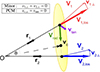 |
Fig. 1. Relative motion of two galaxies, labeled galaxy 1 and galaxy 2. The vector v1 (v2) represents the velocity of galaxy 1 (galaxy 2). The angle θ is measured between r1 and the line connecting the two galaxies. vc is the LoS velocity of the CoM of the pair. The assumptions for different infall models are shown in the top left. |
One assumption is that the perpendicular velocities are low, v2, ⊥ = v1, ⊥ = 0, which is often called the minor infall model. This is essentially a minimal model where only the actual observed LoS velocities are considered and the other components are assumed to be negligible. In this case, vrad can be written as
 (2)
(2)
where  is the ratio between the distance to the galaxy (ri) and the 3D distance between the galaxies (r12).
Another assumption is that the barycenter of the galaxy pair has only a LoS component, i.e., vc, ⊥ = 0. Using the mass ratio of the galaxies, which determines the center of mass (CoM) on the sky, we get the projection CoM (PCM) infall model:
 (3)
(3)
where  . The advantage of this projection is the lack of the dependence of the v⊥.
The PCM model uses the unknown ratio of the two masses, and applying the model requires employing a prior assumption on the probability of that ratio. These assumptions are oversimplified since the dynamics are likely more complicated. However, since tangential motions are impossible to measure, we made these assumptions for the sake of simplicity.
3. Mass determination
3.1. Data and relative motion
Both galaxies, Cen A and M 83, have a large number of distance measurements derived via various methods. We chose to use homogeneous data from the color-magnitude diagrams and the Tip of the Red Giant Branch Distance Catalog (Anand et al. 2021) of the Extragalactic Distance Database (EDD; Tully et al. 2009), which are based on the old stellar population as standard candles. The high-precision distance moduli of  and
and  for Cen A and M 83, respectively, were obtained using Hubble Space Telescope observations with the Advanced Camera for Surveys. As the best heliocentric velocities, we used the optical measurement of vhel = 547 ± 5 by Strauss et al. (1992) for Cen A, which perfectly matches the radio data in EDD, 547 ± 20 (Courtois et al. 2009); and vhel = 518.0 ± 2.6 for M 83, which was measured with high spectral and spatial resolution as part of the HI Nearby Galaxy Survey (THINGS; Walter et al. 2008). Heliocentric velocities were converted to the LG barycenter using the solar apex vector (Makarov et al. 2025), determined from an analysis of the Hubble flow in the vicinity of the LG. Data for Cen A and M 83 are systematized in Table 1.
Data used in this study.
Both mass models were applied to the distances and LoS velocities in the LG barycenter reference frame of the two dominant galaxies in the Cen A/M 83 system. The TA mass of the system was assessed by performing Monte Carlo realizations of the uncertainties on the distances and the LoS velocities as provided in the database. The errors on the distance moduli were assumed to be normally distributed. The application of the PCM model requires an assumption on the unknown mass ratio, which we adopted from the K-band luminosity of the two galaxies (Karachentsev & Kashibadze 2021).
Figure 2 and Table 2 illustrate the distributions of inferred distances and infall velocities derived from the data in Table 1. Both models robustly constrain the radial component of the relative velocity, vrad, to a notably small magnitude. The PCM suggests that Cen A and M 83 could have a negative radial velocity. Such a low-velocity regime is consistent with scenarios in which the galaxies are loosely bound or evolving quasi-independently. While Karachentsev et al. (2007) argued for a positive radial velocity as indicated by the minor infall, our application of the PCM assumption predicts a possible negative radial velocity, providing the first evidence that this system is gravitationally bound and infalling.
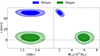 |
Fig. 2. Inferred quantities for the Cen A–M83 radial motion. |
3.2. TA mass and simulation inference
The various versions of the TA model have been tested with the AbacusSummit simulation (Maksimova et al. 2021). This fits our task particularly well since it includes a high-resolution run with particle masses of mpart = 2 × 10⁹ h−1 M⊙ within a large simulation box of 2 Gpc h−1 size for multiple cosmological models. Here we used the data for the fiducial Planck 2018 cosmology (Planck Collaboration VI 2020). The resulting z = 0 halo catalog contains approximately 12 × 106 halos with masses above 1011 M⊙, identified via a spherical overdensity finder applied after a friends-of-friends grouping (Maksimova et al. 2021). The pair-finding algorithm selects halos with masses between 5 × 10¹¹ and 5 × 10¹³ M⊙ and associates each with a single, more massive neighbor. A halo qualifies as a valid partner if it lies within 2 Mpc in 3D separation and if no third halo with Mhalo ≥ 1011 M⊙ is located closer than the chosen companion. To avoid duplication, each halo was allowed to be part of only one pair. Additionally, the relative radial velocity between the two halos must not exceed the Hubble-flow velocity (about 100 km s−1) for the CenA/M83 pair.
To model the velocity components, we used the radial velocity using both the minor and PCM infall assumptions. The tangential velocity (vtan) was sampled via the distribution of β = vtan/|vrad| measured from the cosmological analogs. We tested the TA against the analog pairs under the ideal assumption of exact knowledge of separation and relative velocity, as in Li & White (2008). Solving Eq. (1) for the separation and with the radial velocity giving the TA predicted mass, the minor infall model yields a low TA mass of (2.1 ± 0.5)⋅1012 M⊙ and the PCM a higher TA mass of (6.0 ± 1.2)⋅1012 M⊙.
Simulation-informed correction (M200/MTA) was applied to account for the systematics inherent to the TA method. Figure 3 shows the corresponding correlation between TA masses and the virial masses of the simulation-based analogs. The minor infall solution, representing an unbound or loosely bound configuration, yields a mass of (1.21 ± 0.65)×1012 M⊙, whereas the PCM model predicts a significantly higher value of (6.36±1.31) × 1012 M⊙.
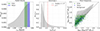 |
Fig. 3. Kinematic properties of the simulated pair sample. The panels show the radial velocity cuts used to define the PCM (green) and minor (blue) candidates (left); the velocity anisotropy distribution (middle); and the resulting MTA vs. M200 relation for each group (right). |
There are cases where the TA crosses the 1:1 correlation (Li & White 2008) and in other cases introduces some bias (Hartl & Strigari 2022; Benisty et al. 2022), which depends on the phase space selection (the radial the tangential velocity ranges). However, in our case statistics allowed for the 1:1 correlation when the radial velocity was much lower then the Hubble flow (PCM), and the minor infall introduces larger biases (see Table 3).
Ratio of the simulation-based mass to the TA mass (left) vs. the final TA + simulation inference mass (right).
The K-band luminosity-to-mass relation, i.e., Eq. (8) from Kourkchi & Tully (2017), provides an independent constraint. Adopting the 2MASS K-band luminosities from Table 1, we obtained a combined mass of Mtotal = (8.26 ± 1.18)⋅1012 M⊙. Virial analyses of the Cen A subgroup and the M 83 subgroup (Karachentsev et al. 2007) yield a combined system mass of (6.0 ± 1.4)⋅1012 M⊙. Multi-Unit Spectroscopic Explorer satellite observations yielded a M 83 subgroup total mass of  (Müller et al. 2025), and Faucher et al. (2026) find (7±2) ⋅ 1012 M⊙, which is consistent with our PCM mass estimates. The Hubble-flow fit yields lower masses of about ∼2 ⋅ 1012 M⊙ (Peirani & Pacheco 2008; Del Popolo & Chan 2022; Faucher et al. 2026), similar to our minor infall estimator. As Faucher et al. (2026) show, the mass based on the Hubble flow method is biased low since the M 83 galaxy is located too close to the turnaround of the system, and in such a case the Hubble flow fit model breaks.
4. Discussion
This work presents the first application of the TA to the Cen A–M83 system, providing an independent dynamical mass constraint for this nearby galaxy pair. The PCM relative motion predicts a mass of MTA, major = (6.36 ± 1.31)⋅1012 M⊙, with an infall velocity of  km s−1. When placed in the broader context of other mass estimators (Fig. 4), the PCM mass is fully consistent with both virial mass determinations and K-band luminosity-based estimates, which cluster around [6–9]⋅1012 M⊙.
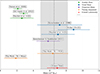 |
Fig. 4. Total mass estimates for the Cen A–M 83 galaxy system from the virial, projected mass, Hubble-flow, and TA methods. The PCM solution agrees well with dynamical and stellar-based estimates, while the minor solution aligns more closely with Hubble-flow prediction. |
Backward integration of the TA equations, using a K-band luminosity mass prior, yields a present-day radial velocity (vrad) of −31 ± 51 km s−1, which favors the PCM scenario. Both TA solutions imply bound or marginally bound orbits. At the observed separation, the Hubble-flow velocity exceeds 100 km s−1, which is significantly higher than either the minor or PCM radial velocity predictions. The corresponding specific orbital energies for the two TA configurations are negative, ϵ ∼ −0.5 ⋅ 103 km2 s−2 (minor) and ϵ ∼ −2 ⋅ 103 km2 s−2 (PCM), confirming that both lie in the bound regime, where ϵ is the total energy per the reduced mass.
The turnaround of the group further reinforces this conclusion (Sandage 1986). The Cen A turnaround radius is estimated to be ∼1.4 Mpc (Karachentsev et al. 2007), only slightly smaller than the current separation of ∼1.5 Mpc. Relative to Cen A alone, M83 may reside just outside the collapsing region, which would allow for a small positive radial velocity, as predicted by the minor infall model. However, if we consider the combined gravitational potential of the full CenA/M83 system, the turnaround radius is larger. Relative to the barycenter, both galaxies lie within the collapsing region, consistent with the PCM prediction of a modest approach speed.
We also address the potential influence of NGC 4945. Although substantial (LK ≈ 0.6LK, Cen A), its dynamical mass is significantly lower (∼20% of Cen A). Located 0.5 Mpc away and on the opposite side of the sky from M83, it forms a tight, bound subsystem with Cen A similar to the LMC–Milky Way pair, which will reduce the predicted mass (Peñarrubia et al. 2016; Benisty et al. 2022; Akib et al. 2025). We therefore consider it to be dynamically associated with the Cen A complex rather than a distinct third body; thus, our derived timing mass encompasses the extended Cen A/NGC 4945 system.
Acknowledgments
We thank Marcel Pawlowski, Jenny Wagner, Yehuda Hoffman and Igor D. Karachentsev for useful discussions. DB is supported by a Minerva Fellowship of the Minerva Stiftung Gesellschaft fuer die Forschung mbH and acknowledges the contribution of the COST Actions CA23130 and CA21136. NIL acknowledges funding from the European Union Horizon Europe research and innovation program (EXCOSM, grant No.101159513). DIM is supported by the Russian Science Foundation grant 24–12–00277.
References
- Akib, I., Hammer, F., & Yang, Y., 2025, A&A, 695, L5 [NASA ADS] [CrossRef] [EDP Sciences] [Google Scholar]
- Anand, G. S., Rizzi, L., Tully, R. B., et al. 2021, AJ, 162, 80 [CrossRef] [Google Scholar]
- Bahcall, J. N., & Tremaine, S. 1981, ApJ, 244, 805 [Google Scholar]
- Banik, I., & Zhao, H. 2016, MNRAS, 459, 2237 [Google Scholar]
- Banik, I., & Zhao, H. 2017, MNRAS, 467, 2180 [NASA ADS] [Google Scholar]
- Banik, I., O’Ryan, D., & Zhao, H. 2018, MNRAS, 477, 4768 [NASA ADS] [CrossRef] [Google Scholar]
- Benisty, D. 2024, A&A, 689, L1 [NASA ADS] [CrossRef] [EDP Sciences] [Google Scholar]
- Benisty, D., & Guendelman, E. I. 2020, Phys. Dark Univ., 30, 100708 [NASA ADS] [CrossRef] [Google Scholar]
- Benisty, D., Vasiliev, E., Evans, N. W., et al. 2022, ApJ, 928, L5 [NASA ADS] [CrossRef] [Google Scholar]
- Chamberlain, K., Price-Whelan, A. M., Besla, G., et al. 2023, ApJ, 942, 18 [CrossRef] [Google Scholar]
- Courteau, S., et al. 2014, Rev. Mod. Phys., 86, 47 [NASA ADS] [CrossRef] [Google Scholar]
- Courtois, H. M., Tully, R. B., Fisher, J. R., et al. 2009, AJ, 138, 1938 [Google Scholar]
- Del Popolo, A., & Chan, M. H. 2022, ApJ, 926, 156 [NASA ADS] [CrossRef] [Google Scholar]
- Faraoni, V., & Jacques, A. 2007, Phys. Rev. D, 76, 063510 [Google Scholar]
- Faucher, A., Benisty, D., & Mota, D. F. 2026, A&A, 705, A112 [NASA ADS] [CrossRef] [EDP Sciences] [Google Scholar]
- Hartl, O. V., & Strigari, L. E. 2022, MNRAS, 511, 6193 [CrossRef] [Google Scholar]
- Karachentsev, I. D., & Kashibadze, O. G. 2006, Astrophysics, 49, 3 [NASA ADS] [CrossRef] [Google Scholar]
- Karachentsev, I. D., & Kashibadze, O. G. 2021, Astron. Nachr., 342, 999 [NASA ADS] [CrossRef] [Google Scholar]
- Karachentsev, I. D., Tully, R. B., Dolphin, A., et al. 2007, AJ, 133, 504 [NASA ADS] [CrossRef] [Google Scholar]
- Kourkchi, E., & Tully, R. B. 2017, ApJ, 843, 16 [NASA ADS] [CrossRef] [Google Scholar]
- Li, Y.-S., & White, S. D. M. 2008, MNRAS, 384, 1459 [CrossRef] [Google Scholar]
- Makarov, D., Makarov, D., Makarova, L., & Libeskind, N. 2025, A&A, 698, A178 [NASA ADS] [CrossRef] [EDP Sciences] [Google Scholar]
- Maksimova, N. A., Garrison, L. H., Eisenstein, D. J., et al. 2021, MNRAS, 508, 4017 [NASA ADS] [CrossRef] [Google Scholar]
- McLeod, M., Libeskind, N., Lahav, O., & Hoffman, Y. 2017, JCAP, 12, 034 [CrossRef] [Google Scholar]
- Mo, H., van den Bosch, F. C., & White, S. 2010, Galaxy Formation and Evolution (Cambridge University Press) [Google Scholar]
- Müller, O., Jerjen, H., & Binggeli, B. 2015, A&A, 583, A79 [NASA ADS] [CrossRef] [EDP Sciences] [Google Scholar]
- Müller, O., Jerjen, H., Pawlowski, M. S., & Binggeli, B. 2016, A&A, 595, A119 [NASA ADS] [CrossRef] [EDP Sciences] [Google Scholar]
- Müller, O., Rejkuba, M., Pawlowski, M. S., et al. 2019, A&A, 629, A18 [Google Scholar]
- Müller, O., Fahrion, K., Rejkuba, M., et al. 2021, A&A, 645, A92 [NASA ADS] [CrossRef] [EDP Sciences] [Google Scholar]
- Müller, O., Rejkuba, M., Fahrion, K., et al. 2025, A&A, 699, A207 [NASA ADS] [CrossRef] [EDP Sciences] [Google Scholar]
- Nandra, R., Lasenby, A. N., & Hobson, M. P. 2012, MNRAS, 422, 2931 [NASA ADS] [CrossRef] [Google Scholar]
- Partridge, C., Lahav, O., & Hoffman, Y. 2013, MNRAS, 436, 45 [Google Scholar]
- Peirani, S., & Pacheco, J. A. D. F. 2008, A&A, 488, 845 [NASA ADS] [CrossRef] [EDP Sciences] [Google Scholar]
- Peñarrubia, J., Ma, Y.-Z., Walker, M. G., & McConnachie, A. 2014, MNRAS, 443, 2204 [Google Scholar]
- Peñarrubia, J., Gómez, F. A., Besla, G., Erkal, D., & Ma, Y.-Z. 2016, MNRAS, 456, L54 [CrossRef] [Google Scholar]
- Planck Collaboration VI. 2020, A&A, 641, A6, [Erratum: Astron. Astrophys. 652, C4 (2021)] [NASA ADS] [CrossRef] [EDP Sciences] [Google Scholar]
- Sandage, A. 1986, ApJ, 307, 1 [NASA ADS] [CrossRef] [Google Scholar]
- Sereno, M., & Jetzer, P. 2007, Phys. Rev. D, 75, 064031 [NASA ADS] [CrossRef] [Google Scholar]
- Strauss, M. A., Huchra, J. P., Davis, M., et al. 1992, ApJS, 83, 29 [Google Scholar]
- Strigari, L. E. 2025, ARA&A, 63, 431 [Google Scholar]
- Tully, R. B., Rizzi, L., Shaya, E. J., et al. 2009, AJ, 138, 323 [NASA ADS] [CrossRef] [Google Scholar]
- van der Marel, R. P., & Guhathakurta, P. 2008, ApJ, 678, 187 [CrossRef] [Google Scholar]
- Wagner, J., & Benisty, D. 2025, A&A, 698, A211 [NASA ADS] [CrossRef] [EDP Sciences] [Google Scholar]
- Walter, F., Brinks, E., de Blok, W. J. G., et al. 2008, AJ, 136, 2563 [Google Scholar]
- Wang, W., Han, J., Cautun, M., Li, Z., & Ishigaki, M. N. 2020, Sci. China Phys. Mech. Astron., 63, 109801 [NASA ADS] [CrossRef] [Google Scholar]
- Zhao, H., Famaey, B., Lüghausen, F., & Kroupa, P. 2013, A&A, 557, L3 [NASA ADS] [CrossRef] [EDP Sciences] [Google Scholar]
Appendix A: Mathematical derivation
To compute the physical separation (r12) between the two galaxies given their angular separation (θ), we used
 (A.1)
(A.1)
where r1 and r2 are the distances of the galaxies from the observer. The geometry and velocity components are illustrated in Fig. 1, showing two galaxies with LoS velocities v1 and v2. The motion of galaxy 2 as seen by galaxy 1 is decomposed into a radial component (vrad) and a tangential component (vtan) such that the full relative velocity is
 (A.2)
(A.2)
Each velocity vector can be written as a combination of three directions: the LoS ( ), the direction perpendicular to the observer-galaxy plane (
 ), and the direction perpendicular to the triangle formed by the observer and the galaxy pair (
 ). For each galaxy i = 1, 2:
 (A.3)
(A.3)
Projecting Eq. (A.2) onto the directions  and
and  , we obtain

where  ,
,  , and
, and  is the projection of the tangential velocity on the O12 plane. These expressions allow us to isolate vrad:
 (A.4)
(A.4)
 (A.5)
(A.5)
When either v1, ⊥ or v2, ⊥ and vtan vanish, these equations simplify. The model assuming v1, ⊥ = vtan = 0 is referred to as the major infall model. The two projection options (onto galaxy 1 or galaxy 2) are not symmetric. Assuming one galaxy has negligible perpendicular and tangential velocities, we can extract both vrad and  :
:
 (A.6)
(A.6)
 (A.7)
(A.7)
In the minor infall model, where v1, ⊥ = v2, ⊥ = 0, only LoS velocities contribute. The radial velocity thus reduces to
 (A.8)
(A.8)
We propose a new model where both galaxies move toward their common CoM. Assuming the CoM has only a LoS component, the velocity is written as
 (A.9)
(A.9)
The position and velocity of the CoM are given by
 (A.10)
where  and
and  . The relative velocities with respect to the CoM are
  and
and  , giving
 (A.11)
Projecting these onto  and
and  gives
gives

 (A.12)
which can be solved for vrad:
 (A.13)
with  . We call this the PCM. For
  , this reduces to the major infall projection on galaxy 1, and for
  on galaxy 2. This projection avoids a dependence on the unobserved perpendicular velocities. The model relies on knowledge of the mass ratio, which must be inferred or marginalized over using priors. The following identities support the analysis.
The unit vector  from galaxy 1 to 2 is
 (A.14)
The directions  and
and  are orthogonal:
 (A.15)
The cosine of the angle θ between either pair of LoS or perpendicular directions is
 (A.16)
Similarly, the sine relations read
 (A.17)
Finally, the projections of  along the LoS and perpendicular directions yield
 (A.18)
 (A.19)
All Tables
Ratio of the simulation-based mass to the TA mass (left) vs. the final TA + simulation inference mass (right).
All Figures
|
Fig. 1. Relative motion of two galaxies, labeled galaxy 1 and galaxy 2. The vector v1 (v2) represents the velocity of galaxy 1 (galaxy 2). The angle θ is measured between r1 and the line connecting the two galaxies. vc is the LoS velocity of the CoM of the pair. The assumptions for different infall models are shown in the top left. |
| In the text | |
|
Fig. 2. Inferred quantities for the Cen A–M83 radial motion. |
| In the text | |
|
Fig. 3. Kinematic properties of the simulated pair sample. The panels show the radial velocity cuts used to define the PCM (green) and minor (blue) candidates (left); the velocity anisotropy distribution (middle); and the resulting MTA vs. M200 relation for each group (right). |
| In the text | |
|
Fig. 4. Total mass estimates for the Cen A–M 83 galaxy system from the virial, projected mass, Hubble-flow, and TA methods. The PCM solution agrees well with dynamical and stellar-based estimates, while the minor solution aligns more closely with Hubble-flow prediction. |
| In the text | |
Current usage metrics show cumulative count of Article Views (full-text article views including HTML views, PDF and ePub downloads, according to the available data) and Abstracts Views on Vision4Press platform.
Data correspond to usage on the plateform after 2015. The current usage metrics is available 48-96 hours after online publication and is updated daily on week days.
Initial download of the metrics may take a while.