| Issue |
A&A
Volume 707, March 2026
|
|
|---|---|---|
| Article Number | A280 | |
| Number of page(s) | 10 | |
| Section | Galactic structure, stellar clusters and populations | |
| DOI | https://doi.org/10.1051/0004-6361/202558783 | |
| Published online | 23 March 2026 | |
MgAl burning chain in M 54: The globular cluster-like properties of a nuclear star cluster
1
Osservatorio Astrofisico di Arcetri,
Largo E. Fermi 5,
50125
Firenze,
Italy
2
Dipartimento di Fisica e Astronomia, Università degli Studi di Bologna,
Via Gobetti 93/2,
40129
Bologna,
Italy
3
INAF, Osservatorio di Astrofisica e Scienza dello Spazio di Bologna,
Via Gobetti 93/3,
40129
Bologna,
Italy
4
INAF, Osservatorio Astronomico di Roma,
Via Frascati 33, 00078 Monteporzio Catone,
Rome,
Italy
★ Corresponding author: This email address is being protected from spambots. You need JavaScript enabled to view it.
Received:
24
December
2025
Accepted:
28
January
2026
Abstract
In this study, we present the chemical abundances of Fe, Mg, Al, Si, and K for a sample of 233 likely member stars of M 54. All the stars were observed with the FLAMES high-resolution multi-object spectrograph mounted at the VLT. Our analysis confirmed the presence of a large metallicity range in M 54, with the majority of the stars having −1.8<[Fe/H]<−1.0 dex and a few stars having [Fe/H]>−1.0 dex. The mean value of the total sample is [Fe/H]=−1.40 (σ=0.22 dex). A Markov chain Monte Carlo analysis revealed that the observed spread in [Fe/H] is compatible with a non-null intrinsic iron dispersion. We also found that the metallicity distribution function and the broadening of the red giant branch of M 54 are not compatible with a single age, but instead suggest a wide age range from ∼ 13 Gyr to ∼ 1−2 Gyr or a smaller age range if a significant He enhancement (Y ∼ 0.35/0.40) is present in the most metal-rich stars. We identified among the stars in M 54 an entire pattern of anticorrelations linked to the MgAl burning cycle. In particular, the metal-rich component displays a higher level of H-burning, with the presence of more extended anticorrelations than the metal-poor component. No Mg-poor ([Mg/Fe]<0.0 dex) stars are identified in M 54. The evidence collected so far cannot be explained by either a globular cluster-like scenario or galactic chemical evolution. The chemical properties of M 54 can be explained within a scenario in which this system formed through the merging of two globular clusters: a metal-poor one with standard characteristics and a more metal-rich one with more pronounced chemical anomalies, possibly younger than the first one. M 54 is confirmed to be a key stellar system for explaining the chemical evolution of a nuclear star cluster.
Key words: stars: abundances / stars: general / stars: low-mass
© The Authors 2026
 Open Access article, published by EDP Sciences, under the terms of the Creative Commons Attribution License (https://creativecommons.org/licenses/by/4.0), which permits unrestricted use, distribution, and reproduction in any medium, provided the original work is properly cited.
This article is published in open access under the Subscribe to Open model. This email address is being protected from spambots. You need JavaScript enabled to view it. to support open access publication.
1 Introduction
Nuclear star clusters (NSCs) are among the densest stellar systems present in the Universe (Walcher et al. 2005; Norris et al. 2014), with masses of ∼ 106 up to 108 M⊙ and half-light radii of about 1−10 pc (Georgiev & Böker 2014; Georgiev et al. 2016). They exhibit structural and stellar-population complexities that point to extended evolutionary histories (see e.g., Neumayer et al. 2020), with age and metallicity spreads, and evidence of prolonged or recurrent star formation (Walcher et al. 2005; Kacharov et al. 2018). The NSCs form through a combination of mechanisms: in situ star formation fueled by gas inflows toward the galactic nucleus, and inspiral and merging of star clusters driven by dynamical friction, with this latter channel preferred in galaxies with M*<109 M⊙ (Neumayer et al. 2020). Determining the relative importance of these channels is essential for understanding the coevolution of NSCs and their host galaxies.
The intrinsically compact nature of NSCs, together with the large distances to most galaxies that host them, generally prevents us from resolving them into individual stars. In this context, two nearby systems represent unique and powerful laboratories: ω Centauri and M 54. They are usually classified as globular clusters (GCs) according to their morphology but exhibit a higher level of complexity (akin to NSCs) than the majority of GCs; for instance, in terms of the intrinsic [Fe/H] spread. Nevertheless, they display some chemical patterns (i.e., Na-O and Mg-Al anticorrelations) that are considered to be distinguishing features of GCs. Both objects are close enough to enable high-precision photometry and spectroscopy of their individual stars, allowing us to examine a NSC (or the relic of one) with a level of detail unattainable for any extragalactic counterpart. This makes them fundamental benchmarks for testing theoretical models of NSC formation and for linking the integrated-light properties of unresolved NSCs to the underlying stellar populations.
While ω Centauri is considered to be the possible remnant of a disrupted dwarf spheroidal galaxy (Bekki & Freeman 2003; Bekki & Tsujimoto 2019), the association of M 54 with an external galaxy is direct: it is embedded at the center of the remnant of the Sagittarius dwarf spheroidal galaxy (Sgr dSph). Sgr dSph is a perfect example of a Galactic satellite that is currently undergoing disruption by the tidal field of the Milky Way (MW; Ibata et al. 1994, 2020; Majewski et al. 2003; Ramos et al. 2022). The central region of Sgr, often referred as the NSC of the galaxy, exhibits a composite stellar population in terms of ages and metallicities, with a bimodal [Fe/H] distribution (Carretta et al. 2010a; Mucciarelli et al. 2017; Alfaro-Cuello et al. 2019), with the two main peaks associated with the red giant branches (RGBs) visible in the color-magnitude diagram (CMD) of Sgr. The metal-poor peak of the [Fe/H] distribution, at [Fe/H] ∼ −1.5/−1.6 dex, is dominated by the old, GC-like system M 54, while the second peak, at [Fe/H] ∼−0.5 dex, corresponds to a Sgr population with ages of ∼ 4−6 Gyr. There is now some consensus on a scenario in which the stellar nucleus of the Sgr dSph galaxy was formed by the concurrence of in situ star formation and the infall of one or more GCs by dynamical friction (Bellazzini et al. 2008; Carretta et al. 2010a; Alfaro-Cuello et al. 2019, 2020). In this paper we refer to M 54 as the bulk of the old and metal-poor population of the Sgr NSC, the one that was considered to be a MW GC until the discovery of the Sgr dSph galaxy, following Bellazzini et al. (2008).
The chemical properties of M 54 further reinforce its somehow dual nature. Its stars exhibit a pronounced spread in [Fe/H] (Bellazzini et al. 2008; Carretta et al. 2010a; Mucciarelli et al. 2017; Alfaro-Cuello et al. 2019), implying a sufficiently deep potential to retain supernova (SN) ejecta and sustain extended chemical evolution, behavior not observed in MW GCs but typical of galactic systems. At the same time, M 54 shows the classic light-element anticorrelations (e.g., Na−O, Mg−Al) characteristic of multiple populations (MPs) in massive GCs (Carretta et al. 2010a; Fernández-Trincado et al. 2021). The chemical anticorrelations observed in all GCs are interpreted as the result of self-enrichment within the cluster (see e.g., Bastian & Lardo 2018), whereby low-velocity material processed through the hot CNO cycle and its secondary NeNa and MgAl chains (e.g., Langer et al. 1993; Prantzos et al. 2007) is incorporated in a subsequent generation of stars. The most accepted theoretical models for the formation of MPs involve the occurrence of at least two episodes of star formation whereby a second generation (SG) of stars, enriched in some elements of the CNO cycle and depleted in others, formed from the material polluted by the first generation (FG) or polluter stars within the first 100−200 Myr of the cluster’s life. Different polluters were proposed in the literature, including intermediate- or high-mass stars in their asymptotic giant branch (AGB) phase (D’Ercole et al. 2010), fast-rotating massive stars (Krause et al. 2013), novae (Maccarone & Zurek 2012; Denissenkov et al. 2014), interacting binary stars (de Mink et al. 2009), and supermassive stars (Denissenkov & Hartwick 2014). All of these polluters fail to completely explain the observed evidence.
The coexistence of a broad iron dispersion together with GClike light-element patterns suggests that M 54 hosts processes commonly associated both with NSCs and with dense cluster formation environments, highlighting its dual nature. These properties make M 54 uniquely valuable for probing the formation pathways of NSCs and for bridging the gap between resolved stellar populations in the Local Group and the unresolved NSCs observed in more distant galaxies.
In this work we present a detailed chemical analysis for 233 likely members of M 54, observed with the high-resolution spectrograph FLAMES@VLT. This paper is organized as follows: in Sect. 2 we present the data, in Sect. 3 we describe the stellar parameters and velocities, in Sect. 4 we detail the analysis, in Sect. 5 we illustrate the results of the abundance analysis, in Sect. 6 we carry out the discussion of the results, and in Sect. 7 we summarize our work.
2 Observations and target selection
The employed spectra were acquired at the Very Large Telescope UT2 (Kueyen) with the optical multi-object spectrograph FLAMES (Pasquini et al. 2002) under the programs 075.D-0075 (PI: Mackey, from July to August 2005), 081.D-0286 (PI: Carretta, from June to September 2009), and 095.D-0539 (PI: Mucciarelli, from July to August 2015). FLAMES/GIRAFFE was employed in the high-resolution mode that allows one to allocate up to 132 fibers simultaneously, while FLAMES/UVES allows one to allocate eight high-resolution fibers.
Within the program 075.D-0075, the GIRAFFE HR21 setup was adopted (R=18000 and a wavelength coverage of ∼ 8484− 9000 Å). Under the program 081.D-0286, two GIRAFFE setups were employed: HR11 (R=29 500 and a wavelength coverage of ∼ 5597−5840 Å) and HR13 (R=26 400 and a wavelength coverage of ∼ 6120−6405 Å). Finally, within the program 095.D0539 the GIRAFFE+UVES combined mode was used. The adopted setups are HR18 (R=20 150 and a wavelength coverage of ∼ 7468−7889 Å), and the UVES Red Arm 580 (R=45 000 and a wavelength coverage of ∼ 4800−6800 Å). All of the setups used allow us to measure Fe, Mg, Al, Si, and K abundances. All the spectra were reduced using the dedicated GIRAFFE and FLAMES/UVES ESO pipelines1, which include bias subtraction, flat-field correction, spectral extraction, wavelength calibration, and (for the UVES fibers) order merging.
All of the used programs sample the spatial region within the tidal radius of M 54; namely, rt=9.868 (Harris 2010). We considered only stars located along the RGB of M 54 (the bluest portion of the RGB of the nuclear region of Sgr), excluding stars belonging to the reddest RGBs (therefore stars younger and/or more metal-rich). The bluest RGB is dominated by M 54, with the old, metal-poor Sgr population superimposed (see Minelli et al. 2023; Liberatori et al. 2025). We discarded stars with a signal-to-noise ratio (S/N) of <20 (mainly stars with G>17) because these spectra do not provide reliable abundances. According to their measured radial velocities (RVs, see Sect. 3.2) and their velocity dispersion profiles, we identified as likely members of M 54 those stars with 120 km s−1 ≲ RV ≲ 170 km s−1, following the procedures described in Bellazzini et al. (2008). At the end, the sample analyzed in this work includes 233 stars. In Table 1 we report the total number of stars analyzed for the different combination of setups. In particular, we analyzed a total of 211 stars from the program 075.D-0075, 42 stars from the program 081.D-0286, and 87 stars from the program 095.D-0539. As we can see from Table 1, the three programs have many stars in common. Figures 1 and 2 show the spatial distribution and the position in the Gaia CMD of the entire sample, respectively.
We inspected the Renormalized Unit Weight Error (RUWE) parameter given by the Gaia catalog for all the targets. According to the Gaia documentation, the RUWE is expected to be around 1.0 for sources where the single-star model provides a good fit to the astrometric observations. The generally adopted threshold value that could indicate that the source is non-single or otherwise problematic for the astrometric solution is 1.4 (Gaia Collaboration 2023, and references therein). In our sample, there are a total of 25 stars with RUWE >1.4 and among them there are nine stars with 2.0< RUWE <4.0. However, we decided to maintain these stars in the dataset as they do not display any significant anomaly in either their RVs or their abundances.
The stars observed with the setups HR11 and HR13 had already been analyzed by Carretta et al. (2010a), while the stars observed with the setup HR18 and in common with Carretta et al. (2010a) were analyzed by Carretta (2022). Also, a total of 83 stars in our dataset are present among the stars analyzed by Bellazzini et al. (2008) with the multi-object spectrographs DEIMOS on the Keck 2 telescope and with the HR21 setup, and among them 37 stars are also found in the dataset analyzed by Carretta et al. (2010a). None of the other stars present in our sample had ever been analyzed before, making this one the largest databases of chemical abundances of M 54 stars based on high-resolution spectra.
Stars observed for different combinations of setups.
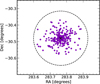 |
Fig. 1 Coordinate positions of the observed targets, displayed with purple circles. The black cross denotes the cluster center (Baumgardt & Hilker 2018). The dashed black circle displays the tidal radius (Harris 2010). |
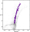 |
Fig. 2 CMD of M 54. Gray points represent the targets associated with Sgr according to the proper motions of Gaia DR3, while the purple circles represent the spectroscopic target stars. |
3 Atmospheric parameters and radial velocities
3.1 Atmospheric parameters
The atmospheric parameters were derived by using the photometric information from Gaia Data Release 3 (Gaia Collaboration 2016, 2023), in order to avoid the spurious effects introduced by the spectroscopic determination of the parameters (Mucciarelli & Bonifacio 2020). We obtained the dereddened (BP−RP)0 color by assuming a color excess factor of E(B− V) =0.15 ± 0.03 (Harris 2010) and adopting the iterative recipe proposed by Gaia Collaboration (2018). We derived the effective temperatures (Teff) for all the targets from the empirical (BP−RP)0−Teff relation by Mucciarelli et al. (2021), calibrated on stars whose temperature was obtained with the infrared flux method. Gaia BP-RP photometry, due to the relatively large apertures adopted, can suffer from contamination in crowded fields (Riello et al. 2021, and references therein). To verify if this affects the temperatures inferred from (BP−RP)0 colors we used the C* parameter, introduced by Riello et al. (2021) as an indicator of the degree of contamination in the BP and RP aperture windows compared to the smaller window used for the G photometry. For 80 stars in our sample with very high C* values, C*>3, we got (V−I) colors from the catalog by Monaco et al. (2002), obtained from PSF fitting photometry. We used the transformations present in the Gaia documentation2 to transform the (V−I) in (BP–RP) color, then we applied the reddening corrections and the Mucciarelli et al. (2021) relations as above to obtain independent estimates of Teff for these 80 stars.
The average differences between the temperatures directly derived from Gaia photometry and those obtained from the transformed magnitudes of Monaco et al. (2002) are ∼ 30 K, which translates into differences in the derived abundances of ∼ 0.02−0.03 dex. We conclude that contamination in the crowded environment of M 54 does not affect (BP−RP) colors and, consequently, our inference of Teff for the target stars in any significant way, for our purpose.
We calculated the internal errors in Teff as the sum in quadrature of the errors due to the uncertainties in photometric data, reddening, and (BP−RP)0−Teff relation. The errors are on the order of ∼ 90−130 K.
To validate our photometric temperatures, we performed a sanity check on the subset of stars with a high number of available Fe I lines (specifically those observed with UVES and the HR11, HR13, HR18, and HR21 setups). For these targets, we derived temperatures via the excitation equilibrium method, which assumes no correlation between the iron abundance, A(Fe), and excitation potential, χ. The spectroscopic temperatures show excellent agreement with the photometric values, with differences typically of ⩽50 K. This corresponds to a negligible impact on derived abundances (∼ 0.04−0.05 dex or less), confirming the reliability of our photometric temperatures for the entire sample.
Regarding the surface gravities (log g) we adopted the Stefan-Boltzmann relation, using the photometric temperature described above and assuming a stellar mass of 0.80 M⊙, according to a BaSTI isochrone with age 13 Gyr and [Fe/H] ∼−1.5 dex (Hidalgo et al. 2018). Stellar luminosities were computed by using the dereddened G-band magnitude, the bolometric corrections by Andrae et al. (2018), and a true distance modulus of (m−M)0=17.10 ± 0.15 mag (Monaco et al. 2004). By propagating the uncertainties in Teff, distance modulus, and photometry we obtained uncertainties in log g on the order of ∼ 0.1.
We derived the microturbolent velocities (vt) from the log g− vt relation provided by Kirby et al. (2009), assuming an error of 0.2 km s−1. We did not determine vt values spectroscopically, in order to avoid large fluctuations, potentially caused by the small number of Fe I lines available for most of the targets. The derived atmospheric parameters, together with additional information, are reported in Table 2.
Data for the target stars belonging to M 54. The adopted solar abundances for the measured chemical elements are from Grevesse & Sauval (1998) and they are reported in the header of each element abundance column.
3.2 Radial velocities
We determined RVs by using the standard cross-correlation technique implemented in the IRAF task FXCOR. Synthetic spectra generated with the SYNTHE code (Sbordone et al. 2004; Kurucz 2005) were employed as template spectra, convolved with a Gaussian profile to reproduce the observed spectral resolution.
When more than one spectrum per star was available, the final heliocentric RV was calculated as the mean of the individual RV values. Table 2 presents the final heliocentric RVs for all targets. The uncertainties reported were calculated as the dispersion of the mean RV normalized to the root mean square of the number of used exposures; when only one spectrum per star was available, we used the error provided by FXCOR.
We checked for possible RV variations among different spectra: only one star, namely #3801447, shows signs of RV variations, with differences of 3 km s−1 and a RUWE =3.73. For all the other stars (including those with RUWE >1.4), the RVs are consistent within the uncertainties.
From the analysis of 233 stars, we derived a final RV mean value of +142.3 ± 0.5(σ=7.8) km s−1. This value is perfectly in agreement with the mean values reported by Carretta et al. (2010a) of +143.7 ± 0.9(σ=8.3) km s−1, and by Bellazzini et al. (2008) of +140.9 ± 0.4(σ=9.3) km s−1. Figure 3 shows the heliocentric RVs of the entire sample as a function of [Fe/H] and the RV distribution represented as a generalized histogram.
4 Abundance analysis
In this work we measured chemical abundances by using our own code SALVADOR (Alvarez Garay et al., in prep.), which performs a χ2 minimization between the line under analysis and a grid of synthetic spectra calculated with the appropriate atmospheric parameters and varying only the abundance of the considered element. We calculated the grids of synthetic spectra by using the SYNTHE code (Sbordone et al. 2004; Kurucz 2005), and by computing one-dimensional, plane-parallel, local thermodynamic equilibrium (LTE) model atmospheres employing the ATLAS9 code (Sbordone et al. 2004; Kurucz 2005) and the new opacity distribution functions of the KOALA database3 (Mucciarelli et al. 2026).
For abundance determination, we performed a thorough linelist selection across the spectral range covered by the used setups, selecting lines that are unblended, unsaturated, and uncontaminated by telluric features at the resolution of the selected setups, respectively. The atomic information for these lines was sourced from the Kurucz-Castelli linelist database4, with some additional updates including the most recent laboratory measurements of log g f available in the literature. For the determination of the abundance ratios, we adopted the solar reference from Grevesse & Sauval (1998).
To determine star-to-star uncertainties associated with the chemical abundances, we used the same approach as the one described in Alvarez Garay et al. (2022). The errors associated with the adopted atmospheric parameters were propagated by recalculating chemical abundances, varying only one parameter at a time (Teff, log g, or vt) by its uncertainty and keeping the other parameters fixed to their best value. Internal errors, associated with the measurement process, were estimated as the line-to-line scatter divided by the root mean square of the number of lines. When only one line was available, such in the case of K, the uncertainties were estimated by resorting to a Monte Carlo simulation. We created synthetic spectra with representative values for the atmospheric parameters of the analyzed stars, and we injected Poissonian noise, according to the S/N of the observed spectra. For each line, we created a total of 200 noisy spectra and derived the abundance with the same procedure used for observed spectra. Finally, we calculated the internal error as the standard deviation of the abundances derived from the 200 simulations.
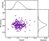 |
Fig. 3 Distributions of the [Fe/H] and RVs for the target stars. The main panel shows the behavior of the RV of the observed stars as a function of [Fe/H]. The generalized histograms of [Fe/H] and RV distributions are also plotted. |
5 Results
In the following subsections, we present in detail the results of the chemical analysis. The derived chemical abundance ratios are reported in Table 2, together with their final uncertainties.
5.1 Iron distribution
Figure 3 shows the metallicity distribution function (MDF hereafter) for the entire sample. The vast majority of stars have an [Fe/H] between −1.8 and −1.0 dex, with only one star with [Fe/H] ∼−2.0 dex and six stars with [Fe/H]>−1.0 dex (the latter is the boundary proposed by Carretta et al. (2010a) to discriminate between M 54 and Sgr stars). The total sample provides an average [Fe/H] of −1.40 ± 0.01 (σ=0.22 dex), while excluding the six stars with [Fe/H]>−1.0 dex and the most metal-poor one, the average value is −1.41 ± 0.01 (σ=0.19 dex). In both cases, the observed dispersion is significantly larger than the typical uncertainties in individual stars, indicating the presence of an intrinsic star-to-star scatter in [Fe/H] among the stars of the blue RGB. To confirm this we used a Markov chain Monte Carlo (MCMC) approach based on the maximum-likelihood principle to assess whether the observed dispersion is compatible with a non-null intrinsic spread in [Fe/H], or whether it can be fully accounted for by the measurement errors. We ran the MCMC analysis both on the full sample of 233 stars and on the subsample of 226 stars with −2.0<[Fe/H]<−1.0 dex. For the complete sample, we obtained a mean value of [Fe/H]=−1.41 ± 0.01 dex and an intrinsic scatter of σint=0.13 ± 0.02 dex, while for the subsample we derived an average [Fe/H]=−1.43 ± 0.01 dex and σint=0.09 ± 0.02 dex. These results indicate that the observed spread in [Fe/H] cannot be fully explained by observational uncertainties but instead is compatible with a non-null intrinsic dispersion. The average [Fe/H] that we found is in good agreement with Bellazzini et al. (2008) (〈[Fe/H]〉=−1.45 dex), while it is ∼ 0.15 and ∼ 0.10 dex higher than the values found by Carretta et al. (2010a) and Mucciarelli et al. (2017), respectively.
Despite M 54 being considered an old stellar system (Siegel et al. 2007), we note that the wide MDF and the relatively narrow RGB in its CMD (see Fig. 2) are not easily compatible with only one age (or a relatively narrow age range of 1−2 Gyr). Stellar isochrones with [Fe/H] ∼−1.0 dex and an age of ∼ 12−13 Gyr should be redder than the RGB of M 54. In order to reproduce the position of the metal-rich stars that we observe along the RGB of M 54, we need to assume younger ages, down to some gigayears. In particular, the position in the CMD of the most metal-rich stars of the sample, with [Fe/H]>−1 dex, is compatible with an age of ∼ 2 Gyr. A similar result has been found by Liberatori et al. (2025), identifying some Sgr field stars (outside the tidal radius of M 54) along the bluest RGB of the galaxy and with [Fe/H] ∼−0.5 dex. These stars are compatible with an age of 1−2 Gyr and can either be stars formed in an additional burst of star formation of the galaxy or the by-products of mass transfer in binary systems. In general, the bulk of the MDF of M 54 (with [Fe/H] between −1.8 and −1.0 dex) seems to imply an age range between ∼ 13 and ∼ 5 Gyr. Such an age range for our sample is consistent with the age-metallicity relation presented by Alfaro-Cuello et al. (2019, see their Fig. 7). However, this age range can be significantly narrowed if we account for a significant He enhancement (Y ∼ 0.35) in the most metal-rich stars. This is clearly shown in Fig 4, where three different BaSTI isochrones5 (Hidalgo et al. 2018) are superimposed on the stars in the CMD. Indeed, by assuming the same age of 12 Gyr for the entire population we can see that the most metal-rich isochrone ([Fe/H]=−1.1 dex) is totally outside the locus of the metal-rich component on the CMD. A more appropriate fit is achieved only by assuming a significantly younger age of ∼ 4−5 Gyr (with Y=0.247) or, alternatively, by keeping an age of 12 Gyr but adopting an enhanced He content of Y ∼ 0.35−0.40.
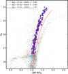 |
Fig. 4 CMD of M 54 with, superimposed, three different isochrones with the same age (12 Gyr) but a different [Fe/H]. The solid cyan isochrone has [Fe/H]=−1.8 dex, the dash-dotted orange isochrone has [Fe/H]=−1.4 dex, and the dashed red isochrone has [Fe/H] = −1.1 dex. |
5.2 Mg, Al, Si, and K distributions
We derived the abundances of those elements involved in the complete MgAl burning chain, in particular, Mg, Al, Si, and K abundances for a total of 155, 50, 45, and 75 stars, respectively. To derive the Mg elemental abundances, we used the Mg line at 5711 Å, the Mg triplet at 6318−6319 Å, and the line at 8806 Å, according to the used FLAMES setup. To derive Al abundances, we used the doublets at 6696–6698 Å and at 7835–7836 Å included in the UVES CD580 and HR18 setups, respectively. To derive Si abundances, we used about 5−10 lines. Finally, the K abundances were derived from the second K I resonance line at 7699 Å6 present in the HR18 setup. In this study we corrected K abundances for the non-LTE effects by interpolating into the grids of Takeda et al. (2002).
Figure 5 shows the distribution of [Mg/Fe],[Al/Fe],[Si/Fe], and [K/Fe] abundance ratios as a function of [Fe/H]. The stars have enhanced values of [Mg/Fe](∼+0.4 dex) until [Fe/H] ∼−1.2 dex and for higher metallicities an overall decrease down to solarscaled [Mg/Fe]. The average value of [Mg/Fe] for the stars with [Fe/H]<−1.2 dex is comparable with that measured in metal-poor Sgr dSph stars not belonging to M 54 (Liberatori et al. 2025). We note a lack of Mg-poor stars in M 54: only three metal-rich stars (∼ 2% of the sample with measured [Mg/Fe]) have subsolar [Mg/Fe] abundance ratios, two of them compatible with the solar value within the uncertainties and one star with [Mg/Fe] ∼ −0.25 dex7.
For the [Al/Fe] distribution, the behavior is the opposite with respect to the [Mg/Fe] distribution. The bulk of the sample exhibits a large star-to-star scatter in [Al/Fe] (from solar value up to ∼+1.3 dex), while the stars with [Fe/H]>−1.2 dex have systematically higher [Al/Fe]. The M 54 stars with lower [Al/Fe] match well the [Al/Fe] abundances of the Sgr stars of similar [Fe/H] (Liberatori et al. 2025), suggesting a similar chemical evolution path, while the stars with higher [Al/Fe] can be considered as SG stars within a GC framework. A small increase with [Fe/H] seems to be visible also for [Si/Fe] but a significantly lower extension. Most of the stars have [Si/Fe] ∼+0.2 dex, while the few metal-rich stars for which we can measure Si abundances have higher [Si/Fe]. Finally, [K/Fe] also shows an increasing run with [Fe/H].
The run of the [Mg/Fe], [Al/Fe], [Si/Fe], and [K/Fe] as a function of metallicity presented here resembles the behavior of both [O/Fe] and [Na/Fe] as a function of [Fe/H] presented by Carretta et al. (2010a) (see their Fig. 15) for the M 54 stars. Indeed, from their analysis it emerges that the most metal-poor stars in their sample have both low and high content of [O/Fe] and [Na/Fe], while the most metal-rich stars are characterized mainly by a high content of [Na/Fe] and low content of [O/Fe]. This seems to also be the case for the [Mg/Fe],[Al/Fe],[Si/Fe], and [K/Fe] distributions in our sample, where our metal-rich component seems to be dominated by the presence of stars with lower (higher) content of Mg(Al, Si, and K) with respect to the metal-poor component.
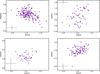 |
Fig. 5 Four panels depicting the distribution of [Mg/Fe] (top left), [Al/Fe] (top right), [Si/Fe] (bottom left), and [K/Fe] (bottom right) as a function of [Fe/H] for the M 54 stars. The error bar in the corner of each panel represents the typical error associated with the measurements. |
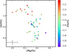 |
Fig. 6 Mg−Al anticorrelation for the stars of M 54. The stars are colorcoded according to their metallicity. The color scale is shown on the right side. The error bar in the bottom left corner represents the typical errors. |
5.3 Mg−Al, Mg−Si, and Mg−K anticorrelations
We measured both Mg and Al abundances for a total of 45 stars in the sample. These stars show a clear Mg−Al anticorrelation (see Fig. 6). Previously, Carretta et al. (2010a) found a hint of Mg−Al anticorrelation from the analysis of six stars, while Fernández-Trincado et al. (2021) detected this anticorrelation in a sample of 19 stars observed within the APOGEE survey (Majewski et al. 2017). The stars with [Fe/H]<−1.4 dex have similar [Mg/Fe] over a large range of [Al/Fe], while the most metal-rich stars have [Al/Fe]>+1 dex and lower [Mg/Fe].
Mg and Si abundances were simultaneously available for a total of 45 stars. All the stars cover a similar range of [Mg/Fe] and [Si/Fe], ranging from ∼ 0.05 to ∼ 0.45 dex. In Fig. 7 we can see the overall Mg−Si anticorrelation among the stars of M 54. A Spearman correlation test provides a correlation coefficient of Cs=−0.29 and a p value of 0.049, enforcing the existence of a real anticorrelation between the two abundance ratios, despite the large uncertainties (∼ 0.15 dex) associated with [Si/Fe]. Similarly to Mg−Al, in this case the most metal-rich stars are those with low [Mg/Fe] and high [Si/Fe]. From Figs. 6 and 7 we can observe that the stars with the higher content of Al are the same as the ones the higher content of Si, and vice versa.
We measured Mg and K abundances simultaneously for a total of 55 stars. Figure 8 shows [K/Fe] as a function of [Mg/Fe]. Indeed, the Spearman correlation test gives Cs=−0.37 and a p value of p=5.3 × 10⁻³, confirming the presence of an anticorrelation between the two abundance ratios.
Among the metal-poor group we found one star, named #3800225, that has [K/Fe]=−0.50 dex, a value that is much lower than all the other stars making the metal-poor component. This star has [Mg/Fe]=+0.52 dex. We tested whether the derived abundance for this star is real or affected by some artifact introduced during the analysis, but we were not able to find any correlation with the adopted stellar parameters. In Fig. 9 we can see the K line for the K-poor star compared with a reference star, named #2421126, which has similar parameters (Teff, log g, vt, and [Fe/H]) but with [K/Fe]=+0.13 dex; this K line is compatible with the abundances of the bulk of the metal-poor component. We can see an obvious difference in the line depths, which implies a real difference in the derived K abundances. Therefore, we conclude that the derived [K/Fe] for #3800225 is real and not an artifact of the analysis.
The presence of a Mg-K anticorrelation in M 54 was claimed by Carretta (2022), who analyzed 42 stars included in our sample. Our analysis confirms their result but with greater statistical significance. The Spearman correlation test for the entire dataset analyzed by Carretta (2022) provides a p value of 0.05, while the exclusion of the star #3800298 (the only Mg-poor stars in his analysis but with a normal [Mg/Fe] in our study) leads to a p value of 0.08. Our dataset provides a correlation coefficient of Cs=−0.41 and a p value of 1.99 × 10⁻³, while, when the anomalous K-poor star is excluded, the dataset provides a Cs=−0.37 and a p value of 5.27 × 10⁻³, confirming the existence of the Mg-K anticorrelation. The difference in the statistical significance between the two studies (even if based on the same spectra) is mainly due to the adopted vt, which significantly impacts the derived K abundances because of the strength of the K lines.
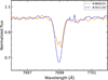 |
Fig. 9 Comparison between the HR18 GIRAFFE spectra of #3800225 (solid orange line) and #2421126 (dashed blue line) stars around the K line at 7699 Å. The depletion of K of #3800225 compared to #2421126 is clearly visible from the comparison. |
6 Discussion
The bluest RGB visible in the CMD of the nuclear region of Sgr is dominated by the GC-like system M 54, with a minor component corresponding to the metal-poor Sgr stars formed in situ (according to the MDF by Minelli et al. (2023), ∼ 14% of the Sgr stars have [Fe/H]<−1.0 dex). The presence of a [Fe/H] spread confirms that the system was able to retain the ejecta from core-collapse SNe, as occurs in complex stellar systems such as galaxies. On the other hand, the presence of anticorrelations forces us to include, in the interpretative framework of M 54, the chemical-enrichment phenomena typically observed in GCs. The existence of a clear Mg-Al anticorrelation in M 54, with stars displaying large variations in the Al abundances, is the signature of Al production through the MgAl chain at very high temperatures (Ventura et al. 2016; Dell’Agli et al. 2018). The Al variations observed cover ∼ 1.5 dex, which is quite large. However, such a value is not surprising, since large variations in the Al abundances are usually found in those GCs very massive and/or metal-poor (Shetrone 1996; Mészáros et al. 2015; Pancino et al. 2017). The presence of the Al−Si correlation is the result of a leakage from the MgAl chain into 28Si through proton-capture reaction at very high temperatures (Yong et al. 2005; Mészáros et al. 2015; Masseron et al. 2019). In the following, we provide a possible interpretative scheme for M 54 able to explain the chemical evidence bridging GCs and NSCs.
6.1 Tentative explanation for the MPs in M 54
Our interpretative scenario for the formation of MPs in M 54 follows the one proposed by Carretta et al. (2010a) to explain their results for the Na-O anticorrelation. Indeed, both in Carretta et al. (2010a) and in this work, the metal-rich component is dominated by SG stars with low content of O and Mg and high content of Na, Al, Si, and K, while the metal-poor component hosts stars with both low and high abundances of these elements. These findings make the anticorrelations more extended at higher metallicities, indicating a higher level of processing by proton-capture reactions in this metallicity regime.
In this scenario the series of events that led to the formation of the different groups of stars in M 54 started with the formation of the most metal-poor stellar component, followed by the formation of the metal-rich stars, which occurred with a delay of ∼ 10−30 Myr (Carretta et al. 2010a). These are the FG stars of M 54. In this case, while polluter stars of 6–8 M⊙ of the metal-poor component evolve into their AGB phase, the massive stars of the metal-rich component continue to explode as core-collapse SNe, preventing the formation of any cooling flow. After the rate of SN explosions becomes low enough, a quiet phase then follows, lasting some tens of millions of years. In this phase, cooling flow formation toward the central regions is possible for both the metal-poor component (with the contribution also from less massive AGB stars of 4−6 M⊙) and the metal-rich one (with AGB stars of 6-8 M⊙, the only polluters that had time to evolve into their AGB phase at this time).
Then, the SG stars form nearly simultaneously in the metal-poor and metal-rich cooling flows. This process lasts until the SN explosion of stars formed in these cooling flows or the onset of type Ia SNe inhibits further star formation. This chain of events is enough to explain the fact that the metal-rich regime is composed of stars with a higher level of Mg depletion and Al, Si, and K enhancement. Indeed, the SG stars of the metal-rich regime formed from the gas of the most massive AGB stars (but without significant Mg depletion as explained in Sect. 6.2), at odds with the SG of the metal-poor component that formed from gas of both massive and less massive AGB stars. Moreover, the SG stars of the most metal-rich population should be enhanced in He (up to Y ∼ 0.35) in order to pacify the observed narrow RGB with the broad MDF.
6.2 The absence of Mg-poor stars in M 54
In M 54 there is no Mg-poor ([Mg/Fe]<0.0 dex) subpopulation, at odds with other systems such as NGC 2419, NGC 2808, NGC 5824, or ω Centauri (Cohen & Kirby 2012; Mucciarelli et al. 2012, 2015, 2018; Alvarez Garay et al. 2024). Apart from ω Centauri, M 54 is the most massive GC. This is an indication that even though the chemical composition of SG stars of M 54 shows up the signature of MgAl processing, the degree of the proton-capture nucleosynthesis activated within the polluter stars was not sufficiently high to allow the ∼ 1 dex depletion of Mg observed in ω Centauri (Alvarez Garay et al. 2024).
In the theoretical framework of the AGB and super-AGB stars, sufficiently advanced proton-capture nucleosynthesis, able to trigger significant depletion of the original Mg, occurs in 4−8 M⊙ stars of metallicities on the order of [Fe/H] ∼−2 dex or less. In higher-metallicity environments such an advanced nucleosynthesis is expected only in AGB stars of mass 6−8 M⊙. In the latter case, in order to form Mg-poor stars in GCs it is a requirement that the formation of SG stars should have taken place directly from the gas released by M ≥ 6 M⊙ stars into the intracluster medium, within a time interval on the order of ∼ 100 Myr. If the formation of the SG extends over a longer period, the interstellar medium would be subsequently enriched by gas from 4−5 M⊙ AGB stars that evolve more slowly and whose nucleosynthesis experienced at the base of the envelope, while sufficiently advanced to favor a factor of ten or more increase in the Al content, is not extreme enough to destroy significant amounts of Mg (Dell’Agli et al. 2018). Therefore, the formation of SG stars with very low Mg content is easier in metal-poor environments, provided that the SG is formed directly from the AGB ejecta, with no dilution with pristine gas, which has the same chemical composition of FG stars.
On the basis of these arguments, the lack of stars with very low [Mg/Fe] values ([Mg/Fe]<0.0 dex) in M 54 is not surprising. While the iron distribution of ω Centauri exhibits a primary peak in the metal-poor domain, at [Fe/H] ∼−1.8 dex (Johnson & Pilachowski 2010; Alvarez Garay et al. 2024), the results shown in Fig. 3 outline the absence of an extended tail to the metal-poor regime in M 54: this indicates that the formation of SG stars with very low Mg was much easier in ω Centauri than in M 54. In the latter cluster Mg-poor stars could form only (1) in the case in which rapid star formation occurred, or (2) directly from the gas released by massive AGB stars of metallicity [Fe/H] ∼−1.9 dex, which evidently was not the case.
For the Al things are slightly different, because the temperatures required for the Al synthesis, on the order of 50 MK, are less extreme than those required for the Mg destruction, which are slightly below 100 MK (Dell’Agli et al. 2018). This is because the Al content of stars is ∼ 50 times smaller than Mg, and thus even proton-capture reactions by the less abundant 25Mg and 26Mg isotopes of Mg, whose activation requires temperatures significantly cooler than the more abundant 24Mg, are sufficient to favor an increase in the Al content of 1 dex or more. This means that a significant increase in Al (e.g., by ∼ 1 dex in [Al/Fe]) can occur even at moderately low metallicities ([Fe/H] ∼−1.3 /−1.2 dex), without a corresponding large decrease in [Mg/Fe].
Finally, the modest increase in [Si/Fe] and [K/Fe] can be explained by the fact that in M 54 the Mg is not processed at levels that allow for a significant Si and K production through the secondary chain of the MgAl cycle, at odds with other systems such as NGC 2419 or ω Centauri: both channels demand temperatures in excess of 100 MK, which are reached only by metal-poor AGBs. Obviously, this scenario requires an appropriate timing for the gas expulsion from the FG stars and the subsequent formation of the SG.
6.3 M 54: A complex cluster
In this work we are focusing on the dominant old and metal-poor population of the NSC lying at the center of the Sgr dSph galaxy. For historical reasons we refer to this component as M 54; however, it is known from the literature as well as from the results presented here that this component is different from the younger and more metal-rich population of the Sgr nucleus, both from a kinematic and from a chemical abundance point of view (Bellazzini et al. 2008; Carretta et al. 2010a,b; Alfaro-Cuello et al. 2019). Within this framework, in the previous sections we showed once again that it displays the chemical patterns typical of MPs observed in GCs and a metallicity spread that is instead typical of galaxies (Willman & Strader 2012). The similarity with ω Centauri was noted long ago (Bellazzini et al. 2008; Carretta et al. 2010b). Indeed ω Centauri is generally believed to be the nuclear remnant of a disrupted dwarf galaxy (see, e.g., Bekki & Freeman 2003; Bekki & Tsujimoto 2019, and references therein).
In this context, we can interpret M 54 following the scenario proposed by Alvarez Garay et al. (2024) for ω Centauri; that is, the merging of two or more GCs plus some contamination from the in situ nuclear population, an idea already put forward by Alfaro-Cuello et al. (2019) for M 54. In this view M 54 should have formed by the merging of two GCs with not very different mean metallicities. Indeed, the MDF of M 54 is asymmetric (see Fig. 3), but it cannot be resolved into two distinct components with the extant data. The most metal-poor progenitor GC is the dominant component of M 54 and it behaves as a normal GC with intermediate properties, a modest Mg depletion and a significant enhancement of Al. The second, less dominant and more metal-rich GC has a larger Mg depletion and a stronger Al enhancement. The two original GCs could had different ages, in order to reconcile the narrow RGB of M 54 with the broad MDF, or similar ages if we assume an important He enhancement in the second cluster, although this latter option seems unlikely.
As was stated, a similar hypothesis has been suggested by Alfaro-Cuello et al. (2019) using low-resolution MUSE data for the nuclear region of Sgr. They found a broad MDF (σ=0.24 ± 0.01 dex) for what they called old and metal-poor component of Sgr (and corresponding to M 54 in our nomenclature) and an age spread of about 1 Gyr, similar to what we argued according to high-resolution spectroscopy and Gaia photometry.
From the work of Bekki & Tsujimoto (2016) it emerged that the presence of so-called “anomalous” GCs, i.e., those massive systems displaying both MPs and large spreads in metallicity, can be explained by the merging of GCs. They performed numerical simulations and several tests and found that the merger between GCs more massive than 3 × 10⁵ M⊙ are inevitable within a host dwarf galaxy with a mass in the range between 3 × 10⁹ M⊙ and 3 × 10¹⁰ M⊙. The dark halo of the progenitor of the Sgr dSph is believed to lie in this mass range (Niederste-Ostholt et al. 2012; de Boer et al. 2014; Gibbons et al. 2017), providing a favorable environment for the GC merging scenario. The infall of these massive clusters is driven by dynamical friction on a scale of a few gigayears. The consequent orbital decay may also favor the merging by bringing both clusters close to the center, or they may both reach the center at different epochs and merge there (see also Gavagnin et al. 2016). In summary, the merging scenario could explain (1) the high mass of M 54, (2) its wide MDF, and (3) its possible age spread. A possible observational test for this scenario would be to look for a bimodal distribution in [Fe/H]. For a given sample, the power of this test would be defined by the precision of individual [Fe/H] measures, which should be significantly better than the 0.1−0.2 dex achieved in this work.
7 Summary and conclusions
We present the largest dataset (233 stars) of high-resolution spectra for RGB stars belonging to the bluest RGB of the nuclear region of Sgr dSph and usually associated with the GC-like system M 54. The main results are summarized as follows:
We confirmed the wide MDF of M 54, with the bulk of the stars having [Fe/H] between −1.8 and −1.0 dex and the presence of a few stars with [Fe/H]>−1.0 dex. An MCMC approach provides [Fe/H]=−1.41 ± 0.01 dex and an intrinsic scatter of σint=0.13 ± 0.02 dex for the complete sample, and [Fe/H]=−1.43 ± 0.01 dex and σint=0.09 ± 0.02 dex considering only the stars with −2.0<[Fe/H]<−1.0 dex. The MDF appears asymmetric but with the current data we are unable to resolve multiple possible peaks.
The MDF and the broadening of the RGB in the CMD are not compatible with a single, old age. A large age range, from ∼ 13 to ∼ 1−2 Gyr, is necessary to reproduce the RGB width, or alternatively a small age range but with a significant enhancement of He (at least for the most metal-rich stars).
In M 54 the complete pattern of anticorrelations linked to the MgAl burning chain is evident. In particular, the most metal-rich component displays a higher level of processing by proton-capture reactions. Indeed, the metal-rich component of M 54 has systematically lower [Mg/Fe] and higher [Al/Fe], [Si/Fe], and [K/Fe] compared to the metal-poor component.
We identified a single K-poor star in M 54, #3800225, exhibiting [K/Fe]=−0.50 dex, a value significantly lower than the bulk distribution for stars with similar parameters. As the star displays no other apparent chemical anomalies, and the current dataset (HR18 and HR21 spectra) is insufficient for a detailed characterization, we postpone a comprehensive analysis of this peculiar object to future work.
The properties of M 54 cannot be explained by either a GC-like scenario or galactic chemical evolution. The observed chemical patterns are compatible with a scenario in which M 54 formed through the merging of two GCs (not resolved in the MDF due to the uncertainties of individual stars), the metal-poor one with standard characteristics and the more metal-rich one with more pronounced chemical anomalies, possibly younger than the first GC.
In conclusion, M 54 emerges as a very complex system, the chemical enrichment history of which was possibly contributed to by different mechanisms.
Data availability
Full Table 2 is available at the CDS via https://cdsarc.cds.unistra.fr/viz-bin/cat/J/A+A/707/A280
Acknowledgements
Funded by the European Union (ERC-2022-AdG, “StarDance: the non-canonical evolution of stars in clusters”, Grant Agreement 101093572, PI: E. Pancino). Views and opinions expressed are however those of the author(s) only and do not necessarily reflect those of the European Union or the European Research Council. Neither the European Union nor the granting authority can be held responsible for them. A.M. and M.B. acknowledge support from the project “LEGO – Reconstructing the building blocks of the Galaxy by chemical tagging” (PI: A. Mucciarelli) granted by the Italian MUR through contract PRIN 2022LLP8TK_001.
References
- Alfaro-Cuello, M., Kacharov, N., Neumayer, N., et al. 2019, ApJ, 886, 57 [Google Scholar]
- Alfaro-Cuello, M., Kacharov, N., Neumayer, N., et al. 2020, ApJ, 892, 20 [CrossRef] [Google Scholar]
- Alvarez Garay, D. A., Mucciarelli, A., Lardo, C., Bellazzini, M., & Merle, T., 2022, ApJ, 928, L11 [NASA ADS] [CrossRef] [Google Scholar]
- Alvarez Garay, D. A., Mucciarelli, A., Bellazzini, M., Lardo, C., & Ventura, P., 2024, A&A, 681, A54 [NASA ADS] [CrossRef] [EDP Sciences] [Google Scholar]
- Andrae, R., Fouesneau, M., Creevey, O., et al. 2018, A&A, 616, A8 [NASA ADS] [CrossRef] [EDP Sciences] [Google Scholar]
- Bastian, N., & Lardo, C., 2018, ARA&A, 56, 83 [Google Scholar]
- Baumgardt, H., & Hilker, M., 2018, MNRAS, 478, 1520 [Google Scholar]
- Bekki, K., & Freeman, K. C., 2003, MNRAS, 346, L11 [Google Scholar]
- Bekki, K., & Tsujimoto, T., 2016, ApJ, 831, 70 [NASA ADS] [CrossRef] [Google Scholar]
- Bekki, K., & Tsujimoto, T., 2019, ApJ, 886, 121 [NASA ADS] [CrossRef] [Google Scholar]
- Bellazzini, M., Ibata, R. A., Chapman, S. C., et al. 2008, AJ, 136, 1147 [Google Scholar]
- Carretta, E., 2022, A&A, 666, A177 [NASA ADS] [CrossRef] [EDP Sciences] [Google Scholar]
- Carretta, E., Bragaglia, A., Gratton, R. G., et al. 2010a, A&A, 520, A95 [NASA ADS] [CrossRef] [EDP Sciences] [Google Scholar]
- Carretta, E., Bragaglia, A., Gratton, R. G., et al. 2010b, ApJ, 714, L7 [Google Scholar]
- Cohen, J. G., & Kirby, E. N., 2012, ApJ, 760, 86 [Google Scholar]
- de Boer, T. J. L., Belokurov, V., Beers, T. C., & Lee, Y. S., 2014, MNRAS, 443, 658 [NASA ADS] [CrossRef] [Google Scholar]
- de Mink, S. E., Pols, O. R., Langer, N., & Izzard, R. G., 2009, A&A, 507, L1 [NASA ADS] [CrossRef] [EDP Sciences] [Google Scholar]
- Dell’Agli, F., García-Hernández, D. A., Ventura, P., et al. 2018, MNRAS, 475, 3098 [CrossRef] [Google Scholar]
- Denissenkov, P. A., & Hartwick, F. D. A., 2014, MNRAS, 437, L21 [Google Scholar]
- Denissenkov, P. A., Truran, J. W., Pignatari, M., et al. 2014, MNRAS, 442, 2058 [NASA ADS] [CrossRef] [Google Scholar]
- D’Ercole, A., D’Antona, F., Ventura, P., Vesperini, E., & McMillan, S. L. W., 2010, MNRAS, 407, 854 [Google Scholar]
- Fernández-Trincado, J. G., Beers, T. C., Minniti, D., et al. 2021, A&A, 648, A70 [Google Scholar]
- Gaia Collaboration (Prusti, T., et al.,) 2016, A&A, 595, A1 [NASA ADS] [CrossRef] [EDP Sciences] [Google Scholar]
- Gaia Collaboration (Babusiaux, C., et al.,) 2018, A&A, 616, A10 [NASA ADS] [CrossRef] [EDP Sciences] [Google Scholar]
- Gaia Collaboration (Vallenari, A., et al.,) 2023, A&A, 674, A1 [NASA ADS] [CrossRef] [EDP Sciences] [Google Scholar]
- Gavagnin, E., Mapelli, M., & Lake, G., 2016, MNRAS, 461, 1276 [NASA ADS] [CrossRef] [Google Scholar]
- Georgiev, I. Y., & Böker, T., 2014, MNRAS, 441, 3570 [Google Scholar]
- Georgiev, I. Y., Böker, T., Leigh, N., Lützgendorf, N., & Neumayer, N., 2016, MNRAS, 457, 2122 [Google Scholar]
- Gibbons, S. L. J., Belokurov, V., & Evans, N. W., 2017, MNRAS, 464, 794 [NASA ADS] [CrossRef] [Google Scholar]
- Grevesse, N., & Sauval, A. J., 1998, Space Sci. Rev., 85, 161 [Google Scholar]
- Harris, W. E., 2010, arXiv e-prints [arXiv:1012.3224] [Google Scholar]
- Hidalgo, S. L., Pietrinferni, A., Cassisi, S., et al. 2018, ApJ, 856, 125 [Google Scholar]
- Ibata, R. A., Gilmore, G., & Irwin, M. J., 1994, Nature, 370, 194 [Google Scholar]
- Ibata, R., Bellazzini, M., Thomas, G., et al. 2020, ApJ, 891, L19 [NASA ADS] [CrossRef] [Google Scholar]
- Johnson, C. I., & Pilachowski, C. A., 2010, ApJ, 722, 1373 [NASA ADS] [CrossRef] [Google Scholar]
- Kacharov, N., Neumayer, N., Seth, A. C., et al. 2018, MNRAS, 480, 1973 [Google Scholar]
- Kirby, E. N., Guhathakurta, P., Bolte, M., Sneden, C., & Geha, M. C., 2009, ApJ, 705, 328 [NASA ADS] [CrossRef] [Google Scholar]
- Krause, M., Charbonnel, C., Decressin, T., Meynet, G., & Prantzos, N., 2013, A&A, 552, A121 [NASA ADS] [CrossRef] [EDP Sciences] [Google Scholar]
- Kurucz, R. L., 2005, Mem. Soc. Astron. It. Suppl., 8, 14 [Google Scholar]
- Langer, G. E., Hoffman, R., & Sneden, C., 1993, PASP, 105, 301 [NASA ADS] [CrossRef] [Google Scholar]
- Liberatori, A., Alvarez Garay, D. A., Palla, M., et al. 2025, A&A, 699, A356 [NASA ADS] [CrossRef] [EDP Sciences] [Google Scholar]
- Maccarone, T. J., & Zurek, D. R., 2012, MNRAS, 423, 2 [NASA ADS] [CrossRef] [Google Scholar]
- Majewski, S. R., Skrutskie, M. F., Weinberg, M. D., & Ostheimer, J. C., 2003, ApJ, 599, 1082 [NASA ADS] [CrossRef] [Google Scholar]
- Majewski, S. R., Schiavon, R. P., Frinchaboy, P. M., et al. 2017, AJ, 154, 94 [NASA ADS] [CrossRef] [Google Scholar]
- Masseron, T., García-Hernández, D. A., Mészáros, S., et al. 2019, A&A, 622, A191 [NASA ADS] [CrossRef] [EDP Sciences] [Google Scholar]
- Mészáros, S., Martell, S. L., Shetrone, M., et al. 2015, AJ, 149, 153 [Google Scholar]
- Minelli, A., Bellazzini, M., Mucciarelli, A., et al. 2023, A&A, 669, A54 [NASA ADS] [CrossRef] [EDP Sciences] [Google Scholar]
- Monaco, L., Ferraro, F. R., Bellazzini, M., & Pancino, E., 2002, ApJ, 578, L47 [Google Scholar]
- Monaco, L., Bellazzini, M., Ferraro, F. R., & Pancino, E., 2004, MNRAS, 353, 874 [NASA ADS] [CrossRef] [Google Scholar]
- Mucciarelli, A., & Bonifacio, P., 2020, A&A, 640, A87 [NASA ADS] [CrossRef] [EDP Sciences] [Google Scholar]
- Mucciarelli, A., Bellazzini, M., Ibata, R., et al. 2012, MNRAS, 426, 2889 [Google Scholar]
- Mucciarelli, A., Bellazzini, M., Merle, T., et al. 2015, ApJ, 801, 68 [Google Scholar]
- Mucciarelli, A., Bellazzini, M., Ibata, R., et al. 2017, A&A, 605, A46 [NASA ADS] [CrossRef] [EDP Sciences] [Google Scholar]
- Mucciarelli, A., Lapenna, E., Ferraro, F. R., & Lanzoni, B., 2018, ApJ, 859, 75 [NASA ADS] [CrossRef] [Google Scholar]
- Mucciarelli, A., Bellazzini, M., & Massari, D., 2021, A&A, 653, A90 [NASA ADS] [CrossRef] [EDP Sciences] [Google Scholar]
- Mucciarelli, A., Bonifacio, P., & Lardo, C., 2026, A&A, 705, A134 [NASA ADS] [CrossRef] [EDP Sciences] [Google Scholar]
- Neumayer, N., Seth, A., & Böker, T., 2020, A&A Rev., 28, 4 [Google Scholar]
- Niederste-Ostholt, M., Belokurov, V., & Evans, N. W., 2012, MNRAS, 422, 207 [NASA ADS] [CrossRef] [Google Scholar]
- Norris, M. A., Kannappan, S. J., Forbes, D. A., et al. 2014, MNRAS, 443, 1151 [NASA ADS] [CrossRef] [Google Scholar]
- Pancino, E., Romano, D., Tang, B., et al. 2017, A&A, 601, A112 [NASA ADS] [CrossRef] [EDP Sciences] [Google Scholar]
- Pasquini, L., Avila, G., Blecha, A., et al. 2002, The Messenger, 110, 1 [Google Scholar]
- Prantzos, N., Charbonnel, C., & Iliadis, C., 2007, A&A, 470, 179 [CrossRef] [EDP Sciences] [Google Scholar]
- Ramos, P., Antoja, T., Yuan, Z., et al. 2022, A&A, 666, A64 [NASA ADS] [CrossRef] [EDP Sciences] [Google Scholar]
- Riello, M., De Angeli, F., Evans, D. W., et al. 2021, A&A, 649, A3 [NASA ADS] [CrossRef] [EDP Sciences] [Google Scholar]
- Sbordone, L., Bonifacio, P., Castelli, F., & Kurucz, R. L., 2004, Mem. Soc. Astron. It. Suppl., 5, 93 [Google Scholar]
- Shetrone, M. D., 1996, AJ, 112, 1517 [NASA ADS] [CrossRef] [Google Scholar]
- Siegel, M. H., Dotter, A., Majewski, S. R., et al. 2007, ApJ, 667, L57 [NASA ADS] [CrossRef] [Google Scholar]
- Takeda, Y., Zhao, G., Chen, Y.-Q., Qiu, H.-M., & Takada-Hidai, M., 2002, PASJ, 54, 275 [NASA ADS] [CrossRef] [Google Scholar]
- Ventura, P., García-Hernández, D. A., Dell’Agli, F., et al. 2016, ApJ, 831, L17 [Google Scholar]
- Walcher, C. J., van der Marel, R. P., McLaughlin, D., et al. 2005, ApJ, 618, 237 [NASA ADS] [CrossRef] [Google Scholar]
- Willman, B., & Strader, J., 2012, AJ, 144, 76 [Google Scholar]
- Yong, D., Grundahl, F., Nissen, P. E., Jensen, H. R., & Lambert, D. L., 2005, A&A, 438, 875 [NASA ADS] [CrossRef] [EDP Sciences] [Google Scholar]
The isochrones were calculated assuming an age of 12 Gyr, a He content of Y=0.247,[α/Fe]=0.4 dex, and three different [Fe/H]: −1.8, −1.4, −1.1 dex.
The first K I resonance line at 7664 Å is heavily contaminated by telluric lines, and therefore is not possible to use this line to derive K abundances.
Carretta et al. (2010a) identified the target #3800298 as a Mg-poor star, with [Mg/Fe] = −0.49 dex. Our analysis of the same star provides a higher value, [Mg/Fe] = +0.24 dex. For this star only the 6318 Å line is available (at variance with the other stars); because this feature is located on the red wing of a auto-ionization Ca I line, its abundance is extremely sensitive to the local normalization and the correct modeling of the auto-ionization line.
All Tables
Data for the target stars belonging to M 54. The adopted solar abundances for the measured chemical elements are from Grevesse & Sauval (1998) and they are reported in the header of each element abundance column.
All Figures
|
Fig. 1 Coordinate positions of the observed targets, displayed with purple circles. The black cross denotes the cluster center (Baumgardt & Hilker 2018). The dashed black circle displays the tidal radius (Harris 2010). |
| In the text | |
|
Fig. 2 CMD of M 54. Gray points represent the targets associated with Sgr according to the proper motions of Gaia DR3, while the purple circles represent the spectroscopic target stars. |
| In the text | |
|
Fig. 3 Distributions of the [Fe/H] and RVs for the target stars. The main panel shows the behavior of the RV of the observed stars as a function of [Fe/H]. The generalized histograms of [Fe/H] and RV distributions are also plotted. |
| In the text | |
|
Fig. 4 CMD of M 54 with, superimposed, three different isochrones with the same age (12 Gyr) but a different [Fe/H]. The solid cyan isochrone has [Fe/H]=−1.8 dex, the dash-dotted orange isochrone has [Fe/H]=−1.4 dex, and the dashed red isochrone has [Fe/H] = −1.1 dex. |
| In the text | |
|
Fig. 5 Four panels depicting the distribution of [Mg/Fe] (top left), [Al/Fe] (top right), [Si/Fe] (bottom left), and [K/Fe] (bottom right) as a function of [Fe/H] for the M 54 stars. The error bar in the corner of each panel represents the typical error associated with the measurements. |
| In the text | |
|
Fig. 6 Mg−Al anticorrelation for the stars of M 54. The stars are colorcoded according to their metallicity. The color scale is shown on the right side. The error bar in the bottom left corner represents the typical errors. |
| In the text | |
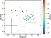 |
Fig. 7 Same as Fig. 6, but for the Mg-Si anticorrelation. |
| In the text | |
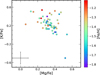 |
Fig. 8 Same as Fig. 6, but for the Mg−K anticorrelation. |
| In the text | |
|
Fig. 9 Comparison between the HR18 GIRAFFE spectra of #3800225 (solid orange line) and #2421126 (dashed blue line) stars around the K line at 7699 Å. The depletion of K of #3800225 compared to #2421126 is clearly visible from the comparison. |
| In the text | |
Current usage metrics show cumulative count of Article Views (full-text article views including HTML views, PDF and ePub downloads, according to the available data) and Abstracts Views on Vision4Press platform.
Data correspond to usage on the plateform after 2015. The current usage metrics is available 48-96 hours after online publication and is updated daily on week days.
Initial download of the metrics may take a while.