| Issue |
A&A
Volume 708, April 2026
|
|
|---|---|---|
| Article Number | A327 | |
| Number of page(s) | 11 | |
| Section | Stellar structure and evolution | |
| DOI | https://doi.org/10.1051/0004-6361/202453460 | |
| Published online | 21 April 2026 | |
Coexistence of internal gravity waves and Tayler-Spruit magnetic fields in the radiative cores of low-mass stars
1
Department of Astronomy, University of Geneva, Chemin Pegasi 51, 1290 Versoix, Switzerland
2
Université Paris-Saclay, Université Paris Cité, CEA, CNRS, AIM, F-91191 Gif-sur-Yvette, France
★ Corresponding author: This email address is being protected from spambots. You need JavaScript enabled to view it.
Received:
16
December
2024
Accepted:
12
March
2026
Abstract
Context. The Tayler-Spruit dynamo (TSD) is capable of generating a small-scale magnetic field in the differentially rotating, stably stratified layers of stars. Its activity was recently observed in numerical simulations. In parallel, the propagation of internal gravity waves in stars can be modified in the presence of a magnetic field.
Aims. We want to estimate the interaction between a magnetic field generated by the TSD and internal gravity waves in the radiative cores of low-mass stars. This allows us to characterise the effect of this interplay on the observed standing mode spectrum and on the internal transport of angular momentum via progressive waves.
Methods. We used the STAREVOL evolution code to compute the structure of low-mass rotating stars with various transport and mixing mechanisms along their evolution. We implemented the formalism to describe the TSD and estimate regions where the magnetic field generated by TSD is strong enough to change the identity of internal gravity waves to magneto-gravity waves. In addition, we evaluated the possible limitation of angular momentum transport via the combined action of rotation and magnetism.
Results. Along the pre-main sequence and main sequence evolution of low-mass stars, the lowest frequencies of the excited gravity wave spectrum should be converted to magneto-gravity waves by the magnetic field generated by the TSD. On the red giant branch, we find that most of the excited spectrum of progressive internal gravity waves could be converted into magneto-gravity waves.
Key words: waves / stars: low-mass / stars: magnetic field / stars: rotation
© The Authors 2026
 Open Access article, published by EDP Sciences, under the terms of the Creative Commons Attribution License (https://creativecommons.org/licenses/by/4.0), which permits unrestricted use, distribution, and reproduction in any medium, provided the original work is properly cited.
This article is published in open access under the Subscribe to Open model. This email address is being protected from spambots. You need JavaScript enabled to view it. to support open access publication.
1. Introduction
The evolution of stellar angular momentum is a fundamental question in astrophysics. The rotation drives a wide variety of physical mechanisms that affects the life of stars (Maeder 2009). Helioseismology (and now asteroseismology overall) allows us to probe the inner regions of the Sun and other stars. In particular, we can estimate the solar rotation profile in its radiative core down to 20% of its radius (e.g. Couvidat et al. 2003; García et al. 2007, 2011; Korzennik & Eff-Darwich 2024). It was found that the rotation profile was very close to solid body, which is indicative of a very efficient redistribution of angular momentum. In addition, thanks to the ability of mixed modes to reach the surface, we are able to retrieve the rotation rate of the inner regions of evolved stars (Beck et al. 2012; Mosser et al. 2012; Deheuvels et al. 2014, 2015; Gehan et al. 2018; Deheuvels et al. 2020; Mosser et al. 2024; Li et al. 2024). Once again, the shallow differential rotation between the core and the surface defies most angular momentum transport models.
The transport of angular momentum in radiative regions has been widely debated and a number of physical processes have been identified over the years in an attempt to explain the rotation profile of the Sun and other type of stars (Charbonneau & MacGregor 1993; Gough & McIntyre 1998; Charbonnel & Talon 2005; Eggenberger et al. 2005; Strugarek et al. 2011; Cantiello et al. 2014; Fuller et al. 2014, 2019; Belkacem et al. 2015; Eggenberger et al. 2019a,b,c; Garaud et al. 2024). While the transport of angular momentum by purely hydrodynamic processes is not efficient enough to explain the rotation profiles measured for the Sun and red giant stars, helio- and asteroseismology have allowed for other mechanisms to be explored (Turck-Chièze et al. 2010; Eggenberger et al. 2012; Ceillier et al. 2012; Marques et al. 2013; Cantiello et al. 2014; Mathis et al. 2018).
On the one hand, stellar interiors are likely magnetised. When they are combined with a mild differential rotation, Maxwell stresses have been shown to efficiently redistribute angular momentum even with low magnetic fields (Mestel & Weiss 1987; Mestel et al. 1988). Later, Spruit (2002) suggested a loop in which the Tayler instability of an initial azimuthal magnetic field (Tayler 1973) is self-sustained and generates a magnetic field in the stellar radiation zone, even with a mild differential rotation. The corresponding formalism can be implemented in stellar evolution codes (Maeder & Meynet 2004; Heger et al. 2005; Petrovic et al. 2005; Eggenberger et al. 2005, 2019c). In particular, Eggenberger et al. (2005) showed that this instability could explain the efficient transport in the solar interior necessary to match the rotation profile reconstructed from helioseismology. Fuller et al. (2019) suggested a revised prescription where the main difference with Spruit (2002) is the saturation for the Tayler instability. They proposed a different turbulence cascade that would lead to a lower energy dissipation rate and, therefore, to a higher magnetic field amplitude and angular momentum transport. Unfortunately, the transport associated with both formalisms is still insufficient to simultaneously explain the red giant and subgiant rotation profiles (Cantiello et al. 2014; Eggenberger et al. 2019b). Until recently, this Tayler-Spruit dynamo (hereafter, TSD) loop was not observed in MHD simulations (Zahn et al. 2007). Petitdemange et al. (2023) first identified in their simulations a mechanism with very similar properties to the TSD, with a field strength comparable to what is predicted by the formalism defined by Spruit (2002). A year later, Barrère et al. (2025) and Petitdemange et al. (2024) explored the instability over a wider range of parameters and identified branches of the instability that scaled similarly to the prescription by Fuller et al. (2019).
On the other hand, internal gravity waves (IGWs) excited at the interface between convective and radiative layers can propagate in the latter and efficiently carry angular momentum to the location where they are damped (Schatzman 1993; Zahn et al. 1997; Kumar et al. 1999; Talon & Charbonnel 2005; Pinçon et al. 2017). This mechanism can potentially explain the chemical mixing and the rotational profile in the Sun and solar-type stars (Charbonnel & Talon 2005; Talon & Charbonnel 2010). Thus, internal magnetic fields and gravity waves have both offered the potential to explain the rotation profile of the Sun and low-mass stars. Nevertheless, while both mechanisms are expected to be present, their interplay has never been studied systematically along the evolution of these stars.
In this framework, one of the key results of the Kepler mission was that about 40% of studied red giants have a missing part in their spectrum (e.g. García et al. 2014; Stello et al. 2016; Bugnet 2022). The magnetic field has been proposed as the main mechanism to explain these so-called ‘depressed’ stars. Indeed, Fuller et al. (2015) demonstrated that a strong enough magnetic field may trap some of the gravity modes in the inner regions and convert them to Alfvén waves, changing their identity, preventing the modes from travelling back to the surface and a part of the observed spectrum ends up missing as a result.
In this context, several issues have arisen. First, the question of how we can describe the interactions between IGWs and a magnetic field generated by TSD; how they affect the progressive waves and the standing modes along the evolution; and, finally, how efficient the modified waves are shown to be transporting angular momentum.
A great deal of effort has been made in the last decade to study the interaction between waves and a magnetic field. On the theoretical side, we refer to the works by Gough & Thompson (1990), Bugnet et al. (2021), Mathis et al. (2021), Li et al. (2022), and Lignières et al. (2024) where a perturbative approach is used; followed by Rogers & MacGregor (2010), Mathis & de Brye (2011, 2012), Lecoanet et al. (2017), Loi & Papaloizou (2018), Loi (2020a,b), 2021), Dhouib et al. (2022), Rui & Fuller (2023), and Rui et al. (2024) where a non-perturbative approach is used. The conversion mechanism from gravity waves to Alfvén waves (i.e. the change in the identity of the wave) is presented in Fuller et al. (2015) and Rui & Fuller (2023), and confirmed by the simulations of Lecoanet et al. (2017, see also the recent work by David et al. 2025), while the impact on the transport of angular momentum can be found in Mathis & de Brye (2012). In particular, the predicted amplitudes of the critical field at which IGWs are converted in Magneto-GW have already been used to constrain the magnetic field in the cores of red giant and massive stars (Cantiello et al. 2016; Bugnet et al. 2021; Li et al. 2022; Lecoanet et al. 2022).
To study the role of the combined mechanism along the evolution, we decided to follow the description of the TSD by Maeder & Meynet (2004), recently confirmed via numerical simulations by Petitdemange et al. (2023). In this work, we aim to understand the various identity changes of the waves along the structure of evolving stars with a radiative core. We want to estimate the role of each mechanism on the transport of angular momentum and the seismic signature when both IGWs and a TSD coexist in the radiative zone. We first describe the type of waves, the magnetic field properties, and the physics of their interaction in stellar stably stratified radiative regions. In Sect. 3, we detail the application to the case of a Sun-like 1 M⊙ star along its evolution. We then extend the discussion to the case of solar-type stars in Sect. 4 before presenting our conclusions.
2. Physics of the problem
Several timescales are to be considered in a magnetised stably stratified rotating radiative region. First, the buoyancy stabilises the medium following the Brunt-Väisälä frequency, N. Then, unless the star is close to breakup (which we do not consider here), we have the rotation frequency below, 2Ω, with Ω as the rotation rate; finally, as displayed in Fig. 1, the Alfvén frequency, ωA, is generally lowest with
 (1)
(1)
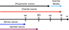 |
Fig. 1. Wave spectrum in a magnetised rotating star. |
where k is the wave vector and VA is the Alfvén velocity defined as  , with ρ and B being the density and the local magnetic field in cgs units, respectively. This leads to several possible types of waves and physical mechanisms occurring in this region. In addition, we assume a weak differential rotation in the latitudinal direction due to anisotropic turbulence and magnetic instabilities (Zahn 1992; Spruit 2002; Mathis et al. 2018).
2.1. Internal gravity waves
Overall, IGWs propagate in stably stratified regions such as the radiative core of solar-type stars with a frequency of ω < N. They are stochastically excited by convective Reynold stresses (Press 1981; Belkacem et al. 2009; Lecoanet & Quataert 2013) and by the penetration of convective plumes in the radiative layers (Rogers et al. 2013; Alvan et al. 2014; Pinçon et al. 2016). The strength of the two excitation mechanisms are comparable all along the evolution in terms of energy injected, but they excite different parts of the wave spectrum. In particular, the energy spectrum is relatively narrow and peaks at low l-degree in the case of an excitation by turbulent convective Reynold stresses, while it is broader and shifted towards higher angular degrees with penetrative convection (see Fig. 8 in Pinçon et al. 2016). The wave spectrum excited by Reynold stresses is expected to peak around the convective turnover frequency while penetrative convection excites all low-frequency waves.
Generally, the excited low-frequency progressive waves are damped by the high thermal diffusivity present in the ambient medium. The dissipation happens at different layers depending on the wave frequency and degree, l, and as they dissipate, the waves also release their energy and angular momentum, thus modifying the stellar interiors properties. However, if the damping of a wave is weak enough, it can undergo reflection leading to the formation of a standing gravity mode, which may then be observed via asteroseismology. The damping of the wave strongly depends on its wavelength (e.g. Zahn et al. 1997). We can thus define a cutoff frequency, ωc, below which the waves are damped too quickly to be able to form standing gravity modes. Alvan et al. (2015) and Ahuir et al. (2021) give
![Mathematical equation: $$ \begin{aligned} \omega _c (r)= \left([l(l+1)]^{3/2}\int _{r}^{R_{\rm rad}} K_T \frac{NN_T^2}{r^3}dr\prime \right)^{1/4}, \end{aligned} $$](/articles/aa/full_html/2026/04/aa53460-24/aa53460-24-eq3.gif) (2)
(2)
where KT is the thermal diffusivity and Rrad is the launching points of IGWs (at the top of the radiative region in our case).
In a rotating star, we may also want to consider the formation of gravito-inertial modes (Dintrans & Rieutord 2000; Prat et al. 2016, 2017, 2018) and progressive waves (Mathis 2009; Augustson et al. 2020), where the influence of rotation through the Coriolis acceleration is no longer negligible. This happens when a wave frequency is of the order of the characteristic rotation frequency (2Ω), as indicated in Fig. 1. In this work, we focus on solar-type stars that are magnetically braked on their main sequence (MS) by the interaction of stellar winds with the large scale magnetic field (Matt et al. 2015); as they are typically slow rotators, as a first step, we can ignore the impact of rotation on gravity waves.
2.2. Tayler-Spruit magnetic field
The turbulent motions in magnetised radiative stellar interiors have been theorised to drive a small-scale dynamo due to the differential rotation. It is born first from the growth of the axisymmetric azimuthal magnetic field driven by shearing flows associated with differential rotation (Spruit 1999). This Ω-effect acts on the large scale poloidal field building a toroidal field. The Tayler instability then onsets as the toroidal field becomes too large (Tayler 1973). Finally, the electromotive force restores the poloidal field, closing the loop (Zahn et al. 2007; Fuller et al. 2019). This leads to the so-called TSD (Spruit 2002).
This dynamo can drive strong magnetic fields in the radiative region of stars and, thus, it holds important consequences for the transport of angular momentum in all type of stars at all stages of evolution (see e.g. Fuller et al. 2019; Moyano et al. 2022, 2023). Recently, Petitdemange et al. (2023) presented the first global numerical simulations, revealing a dynamo with theoretical TSD characteristics, in agreement with Spruit (2002)’s formalism. We note that Fuller et al. (2019) also proposed a formulation from a slightly different dynamo loop, which appears to be too efficient to agree with the results from the simulations by Petitdemange et al. (2023, 2024), although it does agree with some of the simulations by Barrère et al. (2025).
Here, we use a generalised version of the TSD to account for both the thermal and chemical stratification simultaneously, as given by Maeder & Meynet (2004). We refer to Appendix A.1 for the full description of the implementation of the TSD; here, we only recall the expression of the Alfvén frequency in the radial and azimuthal directions.
In the TSD theory, the general Alfvén frequency is given by  , with ρ as the local density. The magnetic field generated by the TSD has a radial (Br) and an azimuthal (Bφ) component with different strengths. In particular, we can show from Maeder & Meynet (2004) that the Alfvén frequencies associated with local azimuthal and radial fields are
 (3)
(3)
with the reduced Brunt-Väisälä frequency  . The full derivation is shown in Appendix A.2, where we assume N ≫ ωA, which is generally the case in stellar radiation zones.
Finally, since ωA, r depends on the frequency, we can define a critical value ωA, r, c, where ω = ωA, r. With the assumption of a strong stratification (N ≫ ωA, N ≫ ω) again (Fuller et al. 2015), we have
![Mathematical equation: $$ \begin{aligned} \omega _{A,r,c} \simeq \omega _A \sqrt{\frac{N}{N_{\rm eff}}}\left[l(l+1)\right]^{1/4}. \end{aligned} $$](/articles/aa/full_html/2026/04/aa53460-24/aa53460-24-eq7.gif) (4)
(4)
2.3. Interactions between IGWs and a magnetic field
2.3.1. Observable signature
García et al. (2014) explored the Kepler data and found a population of red giant stars with reduced (or even missing) mixed modes in their pulsation spectrum, which they associated with the presence of a strong field in the core. Fuller et al. (2015) showed that part of the low-frequency IGWs can convert into Alfvén waves when the strength of the magnetic field is high enough. This should lead to observable consequences on the spectrum of strongly magnetised stars. For example, based on this work, Stello et al. (2016) found that the presence of a magnetic field in the cores of red giants was a strong function of the stellar mass, concluding that the magnetic field was generally a remnant of a convective core dynamo on the MS of intermediate-mass stars. More recently, Bugnet et al. (2021), see also Loi 2021; Mathis et al. 2021; Bugnet 2022; Mathis & Bugnet 2023; Rui et al. 2024; Lignières et al. 2024) computed theoretical asteroseismic signature of a stable axisymmetric and non-axisymmetric fossil field on the stellar oscillation frequency spectrum, allowing for the magnetic field strength in red giant interiors to be estimated. The exercise was performed by Li et al. (2022, 2023), Deheuvels et al. (2023), and Hatt et al. (2024) to detect magnetic field of several tens of thousands of Gauss in the cores of red giant stars and by Lecoanet et al. (2022) in the case of the MS massive star HD43317 with a field of the order of 5 × 10⁵ G.
For MS low-mass stars, IGWs are generally progressive and produced at low frequencies (e.g. Alvan et al. 2014). However, Lecoanet et al. (2017) and Rui & Fuller (2023) showed that when the ambient magnetic field is large enough, gravity waves become evanescent and convert to magneto-gravity waves when their local frequency goes below that of the Alfvén frequency. The mechanism is complex and requires high orders in the WKB development to be reached or to consider modes with a non-harmonic time dependence to fully capture the subsequent spectrum (Rui & Fuller 2023).
2.3.2. Angular momentum transport
The Coriolis and Lorentz forces modify the propagation cavity of the waves and trap them in some parts of a given radiative region. In particular, the consequences on the transport of angular momentum by gravity waves modified by rotation and a toroidal field have been studied by Mathis & de Brye (2012). Following the approach of Talon & Charbonnel (2003), they defined a parameter 𝒫m (Eq. (118) in Mathis & de Brye 2012) to evaluate the fraction of the total momentum flux that is transmitted to waves at the convective-radiative boundary surface, for a fixed excitation rate. We note that in reality, the excited flux is also modulated by the rotation and magnetism (Augustson et al. 2020; Bessila & Mathis 2025). In practice, 𝒫m gives the fraction of the spherical surface at the convective boundary where magneto-gravito-inertial waves are propagative and can be excited. The effective surface where the transmission occurs is reduced due to the combined effects of the equatorial trapping caused by the Coriolis force, and both vertical and equatorial trappings induced by the Lorentz force. The 𝒫m function is expressed as
 (5)
(5)
with
 (6)
(6)
as the control parameter of the system. We also note that as ω < |m|ωA, the waves do not propagate any longer. Although this function was derived for a purely toroidal field, it was shown to give similar trends to the cases with more complex field topologies, which would be closer to realistic conditions (Dhouib et al. 2022; Rui et al. 2024).
For a fixed excitation rate, 𝒫m thus qualitatively estimates the angular momentum flux ratio transmitted at the convective boundary, comparing the rotating case with a toroidal magnetic field with the non-rotating, non-magnetised case. We note that this method is applicable to magneto-Poincaré waves, which reduce to classical IGWs in the non-magnetic, non-rotating case. However, it cannot be applied to Rossby waves (which arise from the conservation of specific vorticity), Yanai waves (mixed gravity–Rossby waves), or Kelvin waves (which result from the combined effects of specific vorticity conservation and stratification) as they have no counterparts in the non-rotating, non-magnetic limit. These specific cases will be addressed in a separate study that is currently in progress, using an approach similar to that adopted by Pantillon et al. (2007) in the non-magnetic rotating case. Mathis & de Brye (2012) also showed that the radiative damping is modified by the Coriolis acceleration and the Lorentz force and, thus, the radii at which the internal waves are damped become closer to the excitation region. As a first step, the present work is therefore focussed on how the latitudinal extent of the cavity of propagation of the waves at the convective-radiative interface affects the transmission of angular momentum from the convective envelope to the radiative core. The evaluation of the role of rotation and magnetism on the radiative damping and on the excitation rate is therefore beyond the scope of this paper. We assume that the transmitted angular momentum flux is deposited before reaching the centre of the star, which provides an estimate of the total torque applied on the radiative core at a fixed excitation rate.
In the following section we assess the impact of a TSD-generated magnetic field on the propagation of gravity waves in a solar-mass star. We place a particular focus on the angular momentum transport using this formalism.
3. Case of a 1 M⊙ star through its evolution
3.1. The stellar evolution model
To compute the structure and the rotational evolution we use the 1D stellar structure and evolution code STAREVOL, which self-consistently computes the evolution of angular momentum (see Siess et al. 2000; Palacios et al. 2003; Decressin et al. 2009; Amard et al. 2019, for a more detailed description of the code). The composition follows Asplund et al. (2009), with the fit from Krishna Swamy (1966) for the atmosphere. The mixing length of αMLT = 2.11 comes from a solar calibration of a non-rotating model. The transport of angular momentum is described with the formalism of Zahn (1992) and Mathis & Zahn (2004), with the horizontal turbulence (along the isobars) being much more important than the vertical one because of the anisotropy of the turbulent transport triggered by the stable stratification (Zahn 1992; Mathis et al. 2018). We treat the meridional circulation as an advective process and all other mechanisms as diffusion terms according to the following equation,
 (7)
(7)
where ρ, r, νv, v, and Ur are the density, radius, vertical component of the turbulent viscosity, and radial component of the velocity of the l = 2 meridional circulation on a given isobar, respectively. We implemented, for the first time in STAREVOL, the transport by the TSD (as described in Appendix A.1) to compute the corresponding diffusivity, νTS. We recall here that both the rotation profile and the magnetic field properties are strongly determined by the chosen prescription, namely, that of Spruit (2002). Finally, the external torque is computed following Matt et al. (2015), calibrated to reach the solar surface rotation rate at the age of the Sun, along with a saturation of the dynamo-generated magnetic field for  ; here, τc and Prot are the convective turnover timescale at HP/2 above the base of the convective region and the surface rotation period, respectively. Finally, we acknowledge that most observables tend to show a weakening of the surface magnetic torque beyond roughly the age of the Sun for solar-like stars (van Saders et al. 2016; David et al. 2022; Bhalotia et al. 2024; Metcalfe et al. 2025). However, we do not expect this to qualitatively affects the results of this paper. Thus, to avoid adding any more parameters to the model, we kept the same expression for the stellar wind torque during the whole evolution.
We ran a 1 M⊙ evolution model with rotation from the early pre-main sequence (PMS) to the red giant branch (RGB). In this section we present the key moments of a star’s life to represent the evolution of the structure and various cavities crossed by typical IGWs excited at the base of the convective envelope. We also computed the fraction of angular momentum that is transmitted by internal waves from the convective envelope to the radiative core using Eq. (5).
In Fig. 3, the red line indicates ωTO, which is the convective turnover frequency at the base of the convective envelope. The wave excitation is expected to be maximal around this value (Press 1981; Fuller et al. 2014). In particular, during the PMS and after the terminal-age main sequence (TAMS), the convective eddies are much larger and peak excitation takes place at lower frequencies. We can distinguish two classes of waves separated by the cut-off frequency (blue shaded region on Fig. 3). Above this value, the waves form standing g-modes. Below the cut-off frequency, the waves are progressive and will dissipate due to thermal diffusion (Alvan et al. 2013), critical layers, or non-linear breaking (Zahn et al. 1997; Mathis 2025). The evolution of the rotation profile under the influence of both hydrodynamical processes (meridional circulation and shear instabilities) and the TSD is presented in Fig. 2. We first confirm the findings of Eggenberger et al. (2005, 2019a) that during the PMS, despite the contraction, the star is very close to solid-body rotation due to the fast rotation and the low stratification of the star which both efficiently trigger the TS instability. It is only during the MS (at an age slightly younger than that of the Sun) that a differential rotation sets in close to the core where the stratification has increased enough to prevent the TS instability. Finally, as the 1 M⊙ star evolves to the subgiant branch (SGB) and rises along the RGB, the differential rotation increases as neither the TSD, nor the hydrodynamical instabilities are efficient enough to extract the concentration of angular momentum in the core associated with the contraction (Cantiello et al. 2014).
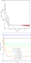 |
Fig. 2. Top: Rotation profile at the age of the Sun for the 1 M⊙ model. The points and their error bars are from Eff-Darwich et al. (2008). Bottom: Rotation profile evolution of the 1 M⊙ model through the ages as indicated on each plot. |
In Fig. 3, we display the frequencies relevant to the characterisation of the wave properties as described in Sect. 2 along the evolution of the 1 M⊙ star. The top three panels present the PMS structure evolution, the central left one corresponds to the solar age, and the remaining ones show the evolution from the TAMS to the RGB stage, as presented in the top-left panel of Fig. 3. Overall, we ought to first verify that we are always in a highly stratified situation, meaning that we are always dominated by the Brunt-Väisälä frequency (black line in Fig. 3). The cut-off frequency, ωc, delimits the regime of stationary g-modes modes (blue shaded region in Fig. 3) from that of progressive IGWs. Its value remains below the Brunt-Väisälä frequency; thus, both types of waves are able to propagate in the radiative region through the evolution.
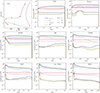 |
Fig. 3. Top-left: Location of each selected profile on the Hertzsprung-Russell diagram of the 1 M⊙ model. The next diagrams show the variations of the relevant characteristic frequencies along the evolution. From top centre to bottom right: Early PMS (5 Myr), Henyey track (25 Myr), ZAMS (52 Myr), solar age (4.57 Gyr), TAMS (9.61 Gyr), SGB (10.53 Gyr), base of the RGB (10.97 Gyr), and middle of the RGB (11.38 Gyr). The light blue region indicates the frequency range of standing gravity modes. |
3.2. Standing gravity modes
Standing gravity modes are built by the constructive interference of IGWs. They are found at frequencies higher than the cutoff frequency, ωc. Since ωc ≥ ωA for the entire evolution depicted here, the modes are not affected by the magnetism generated by the TSD. This goes along with the conclusions of recent work by Fuller et al. (2015) and by Rui & Fuller (2023) that only strong magnetic fields will affect the observable modes. This enforces the conclusion that the magnetic field capable of hindering, retaining, or trapping some of the modes in the cores of red giant stars comes from a fossil magnetic field, and not a TSD mechanism (Bugnet et al. 2021; Li et al. 2022).
3.3. Progressive waves
Progressive waves can follow several possible paths depending on their excited frequency. During the PMS, the fast rotation ensures a strong TSD and, thus, a high Alfvén frequency, ωA, of a few tenths of micro-hertz from the base of the convective envelope to the centre of the star (or the edge of the convective core when present). All the gravity waves excited with frequencies below this value are quickly converted into magneto-gravity waves (MGW) and retain this identity as they propagate to the core. They may locally enhance the torque associated with the magnetic field through Maxwell stresses, here convened by the TSD. All higher frequencies propagate as IGWs and deposit their angular momentum when the thermal diffusion dissipates them, or where they break or encounter a critical layer (see e.g. Talon & Charbonnel 2005; Alvan et al. 2013; Charbonnel et al. 2013; Mathis 2025). At the zero-age main sequence (ZAMS), the 1 M⊙ star has a convective core and the strong chemical gradient above its surface prevents the TSD from maintaining a strong coupling. Locally, this allows for a fast rotation and a higher Alfvén frequency.
On the MS, the convective core has disappeared, but the stratification starts building, limiting the strength of the TSD and slowly increasing the differential rotation in this region, while decreasing the Alfvén frequency below 10 nHz in the core. As we get closer to the convective boundary, the stratification is less important, and the upper half of the radiative region is still driven by the torque from the magnetised stellar wind. Therefore, these layers undergo a higher shear that keeps the local magnetic field generated by the TSD at a high level. It translates into a higher radial Alfvén frequency and thus a larger part of the IGW spectrum excited at the base of the convective envelope can be directly converted in MGW. The interesting part is that after crossing the strongly magnetised region where the TSD is very efficient, the waves may change again their identity as their frequency becomes higher than ωA. The exact state of these waves following this change is not presently clear and we will follow on this discussion in specific papers in the future. The waves of higher frequencies are still propagating as typical IGWs.
As the star reaches the end of the MS, the stratification in the central layers has strongly increased and a chemical gradient has formed from the nuclear reactions. The combination of both stabilising factors locally hinders the TSD and reduces the transport of angular momentum, thus leading to a steep rotation gradient close to the cores of subgiants and red giants, in agreement with Vrard et al. (2022). However, although the TSD is not sufficient to fully couple the central part to the rest of the radiative zone, the strong differential rotation and the faster rotation of the core are able to generate a strong magnetic field and more IGW frequencies can be converted to MGW. For example, in the case of a star at the base of the RGB (central bottom panel on Fig. 3), IGWs with a frequency between 0.01–1 μHz might be able to propagate all the way to the central region around r = 0.01R* (where their frequency becomes comparable to the Alfvén frequency). As discussed in the following subsection, the progressive waves that reach this region should locally release the angular momentum they acquired from the excitation region. They should therefore be accounted for in the transport of angular momentum, as done in Charbonnel et al. (2013) for example. The radial component of the magnetic field is generally associated with a conversion of IGW to MGW (Rui & Fuller 2023), while the horizontal component is associated with a vertical magnetic trapping of the waves (Mathis & de Brye 2011). In each diagram, we show the radial and azimuthal components of the Alfvén frequency in blue and orange, respectively, as computed in Appendix A.1. For most of the evolution, the radial component dominates and low-frequency IGWs should preferably convert to MGWs. At the ZAMS and during the MS, as the core contracts, the azimuthal component becomes slightly higher than the radial one, and IGWs are likely to be vertically trapped as they reach the central regions. However, when the star goes towards the RGB, the effective BV frequency drops as the magnetic diffusivity increases and ωA, r rises again.
On each diagram, the red lines indicate the turnover frequency, which generally corresponds to the peak of excitation by Reynold stresses for IGW (see e.g. Fuller et al. 2014). We advise keeping in mind that a whole spectrum of frequency is excited, which also goes to lower frequencies. In addition, the spectrum excited by penetrative convection could be very important at lower frequencies (Alvan et al. 2014; Pinçon et al. 2016). It is clear from Fig. 3 that along the MS evolution, the IGWs excited by the bulk of Reynold stresses have a characteristic frequency much higher than the Alfvén frequency and should therefore not be affected by the TSD magnetic field. Again, low-frequency IGWs excited by penetrative convection could be affected by the TSD. On the SGB and RGB, the convective envelope quickly deepens so that the convective turnover frequency decreases. Meanwhile, the strong increase of the stratification and the differential rotation in the core leads to higher magnetic field and, thus, to a higher ωA. The bulk of excitation is now comparable to the Alfvén frequency and most of the spectrum of excited IGWs can be converted to MGWs when the star climbs up the RGB. For example, in the last panel, all the waves with a frequency below 1 μHz are converted to MGWs. We note, however, that in our simulations, the core rotation on the RGB is still too high compared to observations by almost an order of magnitude (Cantiello et al. 2014). Therefore, the shear is likely too important and the magnetic field generated as a consequence might be lower.
3.4. Angular momentum transport
In a non-magnetised and non-rotating star, the wave excitation and the transport of angular momentum occur over the whole sphere. However, the rotation contains waves closer to the equator, and the magnetic field prevents the full transmission of angular momentum, both in the vertical and latitudinal directions. We took advantage of the work by Mathis & de Brye (2012) to compute the torque transmitted from the convective envelope to the radiative core in the rotating magnetised case when compared to the one in the non-rotating, non-magnetised one, for a fixed excitation rate1. The exact radius at which the waves are damped is determined mainly by their radiative damping, which is also modified by the Coriolis acceleration and the Lorentz force (Mathis & de Brye 2012). Its evaluation for a given frequency power spectrum will be addressed in a forthcoming work. In the current study, we consider the magnetic field generated by TSD and the rotation profile in the upper 5% in radius of the radiative core to act akin to a filter. We therefore computed the integrated 𝒫m value over this thin layer to estimate the fraction of the flux of angular momentum that is transmitted to the radiative core. Figure 4 shows the 𝒫m factor defined in Sect. 2.3 for m = −1 (i.e. large scale retrograde waves) as a function of the wave frequency and time for the 1 M⊙ star model under the influence of rotation (left), magnetism (centre), and both rotation and magnetism (right).
 |
Fig. 4. Colour maps of the transmission function, 𝒫m, from Mathis & de Brye (2012) with m = −1 as a function of frequency and time for a 1 M⊙ star. Left (centre): 𝒫m when only the rotation (toroidal magnetism) is taken into account. Right: Case with the full contribution coming from 𝒫m. White regions show where the angular momentum flux carried by the wave is unaffected by the rotation and magnetic field while black regions indicate where it is. The dashed part of the diagram present the region where the waves are completely trapped vertically and therefore do not propagate. The red line shows the convective turnover frequency as a function of time, which acts as a proxy for the peak of excitation. The blue and the green lines are the inertial frequency (2Ω) and the Alfvén frequency integrated over the upper 5% of the radiative core, respectively. |
The first notable element is the role of the rotation in the trapping, compared to the magnetic field. The left panel, with rotation only, is indeed very similar to the right panel where both the magnetic field and the rotation are taken into account. In practice, the TSD-generated magnetic field only plays a role in trapping sub-alfvenic waves and so, for the current case, these would include waves with a frequency below 0.01 μHz at most. Therefore, we mainly focus on the role of rotation in this work. We can see that, as soon as the waves become sub-inertial, the trapping is increasing. We also note that we only show the case of retrograde waves where m = −1. The reason is that although 𝒫m depends on the sign of m (Eq. (5)), the difference between two m values of opposite signs varies with ωA2. Therefore, we do not see any visible difference in 𝒫m for prograde and retrograde waves.
We then compared the trapping region with the bulk of the excited spectrum of IGWs, indicated by the red line in Fig. 4. During the early evolution, the combination of the larger envelope first with a low convective turnover frequency, and then the fast rotation leads to a very efficient trapping of the waves with frequencies lower than 7 μHz during the early PMS, and 20 μHz at ZAMS. Around 500 Myr, the star has spun down enough from the magnetised winds that most of the angular momentum carried by IGWs can filter inward to the radiative core. We can therefore expect that angular momentum transport will be more efficient from this point on. During the later evolution, on the one hand, the convective turnover frequency decreases as the convective envelope inflates in the SGB and then the RGB; on the other hand, the rotation rate (and the Alfvén frequency) always remains much smaller, as can also be seen on the last two panels of Fig. 3. This leads to an efficient transmission of the convectively excited angular momentum flux to the inner regions of the star. There, as previously discussed, the IGWs can be converted to magneto-gravity waves close to the core and, thus, the transport of angular momentum would be modified.
4. Other masses with radiative cores
In this section, we present the same evaluation on stars of masses between 0.6 and 1.2 M⊙. Due to their faintness and their low oscillation amplitude, associated with the larger surface variability associated with magnetic activity, the observable counterpart is much more challenging to obtain for stars with a mass lower than the Sun (Verner et al. 2011). However, recent works with ESPRESSO and TESS showed promising results for mid-K dwarfs (Campante et al. 2024; Hon et al. 2024). Therefore, we extended our study to this mass range.
In the top and middle panels of Fig. 5, we show the various frequencies at three different ages for a 0.6 and 0.8 M⊙. As expected, since these stars do not reach evolved phases within the lifetime of the Universe and are even more strongly stratified on the MS, the effect of a magnetic field generated by a TSD on the propagation of IGWs is negligible, as ωTO ≥ ωA for the entire evolution. Because of their convective envelope going much deeper, the convective turnover frequency of the two models reaches lower value on the MS compared to the 1 M⊙ case, even below 1 μHz in the case of the 0.6 M⊙ star. On the ZAMS, the Coriolis frequency is comparable to the effective BV frequency, but the shearing being extremely small, as the effective magnetic field generated by TSD stays on the weaker side. As the stars evolve, they become more stratified and reach slower rotation rates than the Sun; thus, the TSD weakens and the local Alfvén frequency stays way below both the cut-off frequency and the convective turnover frequency until the end of the MS.
We also explored the case of a 1.2 M⊙ star on the MS, presented at the bottom of Fig. 5. Although this type of star has a small convective core for most of the MS, this does not appear to drastically change the pattern we presented in the case of the 1 M⊙ model. In this case, the standing gravity modes are not affected by the TSD on the MS, since the cutoff frequency is again well above the Alfvén frequency. We note that as the star reaches the TAMS, the rotation profile is only mildly differential, confirming the disagreement with asteroseismic observations of the core rotation of subgiant stars that was shown in Cantiello et al. (2014). Regarding progressive IGWs, since we focussed on the MS, ωA stays well below 1 μHz and the convective turnover frequency, showing that a TSD-generated magnetic field has little effect on most of the propagation of progressive gravity waves during the MS of these stars.
We computed the angular momentum transmission function, 𝒫m, for the different masses. It is qualitatively similar to the 1 M⊙ case, but there are some quantitative differences that are mostly due to the different rotational evolution for a given stellar mass. The lower the mass, the longer it takes the star to start spinning down, but the more efficient the spin-down (Matt et al. 2015). This is clearly visible on Fig. 6, where the 0.6 and 0.8 M⊙ stars start to spin down around 100 Myr, while the 1.2 M⊙ stars slow down already after 25 Myr, but the former reach low frequencies, down to 0.5 μHz at 10 Gyr; meanwhile, the latter stay relatively fast (i.e. a few μHz at the end of the MS). In addition, lower-mass stars have a thicker convective envelope and so a longer convective turnover timescale (red line on Fig. 6), the bulk of excited waves is thus at lower frequencies. For the 0.6 and the 0.8 M⊙ cases, most of the angular momentum flux carried by IGWs can be transmitted to the radiative core only after 1 Gyr approximately. Before then, most of the excited flux is clearly sub-inertial and therefore only a very small fraction can be transmitted to the radiative core when compared to the non-rotating non-magnetised case. Although the 1.2 M⊙ star is a faster rotator, its small envelope allows for a higher convective turnover frequency. During the PMS, IGWs at the turnover frequency do not propagate to the core, but starting at ZAMS, 𝒫m increases at the turnover frequency and a good part of the convectively excited flux can cross to the radiative core. Finally, around 300 Myr, most of the IGW flux can be transmitted to the radiative core. We also note that in all cases, the Alfvén frequency remains too small to have an impact on the propagation of the excited waves.
 |
Fig. 6. Same as Fig. 4, but from left to right: Transmission function, 𝒫m, for the 0.6 M⊙, 0.8 M⊙, and 1.2 M⊙ stellar models along their respective evolution, in the case with rotation and magnetism. |
5. Conclusions
In this paper, we investigate the role of a magnetic field generated by a TSD, following Spruit (2002) formalism on the propagation of internal gravity waves in the radiative cores of F-, G-, and K-type stars. We computed the evolution of solar-like stars with rotation from the PMS up to the RGB, including the transport associated with the TSD. While the results strongly depend on the prescription we used to model the dynamo, we show that in the case of a TSD modelled according to Spruit (2002), the produced magnetic field could affect the low-frequency part of the spectrum of progressive gravity waves; in particular, as the star goes up the RGB, but is too weak to affect standing gravity modes. The latter point means that there are no direct observable counterparts. This is because the Alfvén frequencies associated with the TSD magnetic field are far inferior with respect to the cut-off frequencies above which the constructive interference of IGWs sustains standing gravity modes. Therefore, we did not expect the asteroseismic signature to directly capture the TSD, even on the RGB, where it produces the strongest magnetic field. Nevertheless, we point out that it may be of greater importance for the transport of angular momentum during the RGB. At this stage, the peak of internal gravity waves excitation falls in the frequency range expected to be converted to magneto-gravity waves, locally affecting the transport and the rotation profile. This work presents the first application, on stellar structure models, of a formalism designed to compute a transmission function that characterises the trapping of parts of the internal gravity wave spectrum by rotation and magnetic fields. We show that the trapping of low-frequency waves is very important during the early evolution, mostly because of the fast rotation rate of young stars that limits the latitudinal extent of the cavity for a large part of the excited spectrum. In the later stages of the evolution, the wind braking has spun down the stars enough that most of the excited spectrum becomes super-inertial, largely extending the surface through which the IGWs can penetrate in the radiative core to then release their angular momentum. The role of the magnetic field at this stage is very limited since it only applies to waves of extremely low frequencies. However, it is expected to play a role (alongside rotation) in the damping of waves in the radiative zone. This, however, needs to be explored further through some self-consistent computations including TSD, transport by internal gravity waves (which become magneto-gravito-inertial waves), as well as the contribution of the latter to the former. In a follow-up paper, we will explore the case of intermediate-mass stars (e.g. gamma Doradus stars) whose rotation profiles might be retrieved during the MS (Van Reeth et al. 2016; Ouazzani et al. 2017; Christophe et al. 2018; Ouazzani et al. 2019, 2020; Li et al. 2020; Moyano et al. 2023; Aerts et al. 2025) and, thus, additional constraints should be available for such stars.
Acknowledgments
We thank the referee, Jim Fuller, for their insightful comments that clearly improved the manuscript. L.A. and S.M. acknowledge support from the Centre National des Etudes Spatiales (CNES) through SOHO/GOLF and PLATO grants at CEA/Irfu/DAp-AIM. S.M. acknowledges support from the European Research Council (ERC) under the Horizon Europe program (Synergy Grant agreement 101071505: 4D-STAR) and from PNPS (CNRS/INSU). L.A. acknowledges support from the Swiss National Science Foundation (SNF; Project 200021L-231331) and the French Agence Nationale de la Recherche (ANR-24-CE93-0009-01) “PRIMA – PRobing the origIns of the Milky WAy’s oldest stars”. While partially funded by the European Union, views and opinions expressed are however those of the authors only and do not necessarily reflect those of the European Union or the European Research Council. Neither the European Union nor the granting authority can be held responsible for them.
References
- Aerts, C., Van Reeth, T., Mombarg, J. S. G., & Hey, D. 2025, A&A, 695, A214 [NASA ADS] [CrossRef] [EDP Sciences] [Google Scholar]
- Ahuir, J., Mathis, S., & Amard, L. 2021, A&A, 651, A3 [NASA ADS] [CrossRef] [EDP Sciences] [Google Scholar]
- Alvan, L., Mathis, S., & Decressin, T. 2013, A&A, 553, A86 [CrossRef] [EDP Sciences] [Google Scholar]
- Alvan, L., Brun, A. S., & Mathis, S. 2014, A&A, 565, A42 [NASA ADS] [CrossRef] [EDP Sciences] [Google Scholar]
- Alvan, L., Strugarek, A., Brun, A. S., Mathis, S., & Garcia, R. A. 2015, A&A, 581, A112 [NASA ADS] [CrossRef] [EDP Sciences] [Google Scholar]
- Amard, L., Palacios, A., Charbonnel, C., et al. 2019, A&A, 631, A77 [NASA ADS] [CrossRef] [EDP Sciences] [Google Scholar]
- Asplund, M., Grevesse, N., Sauval, A. J., & Scott, P. 2009, ARA&A, 47, 481 [NASA ADS] [CrossRef] [Google Scholar]
- Augustson, K. C., Brun, A. S., & Toomre, J. 2019, ApJ, 876, 83 [Google Scholar]
- Augustson, K. C., Mathis, S., & Astoul, A. 2020, ApJ, 903, 90 [NASA ADS] [CrossRef] [Google Scholar]
- Barrère, P., Guilet, J., Raynaud, R., & Reboul-Salze, A. 2025, A&A, 695, A183 [NASA ADS] [CrossRef] [EDP Sciences] [Google Scholar]
- Beck, P. G., Montalban, J., Kallinger, T., et al. 2012, Nature, 481, 55 [Google Scholar]
- Belkacem, K., Mathis, S., Goupil, M. J., & Samadi, R. 2009, A&A, 508, 345 [NASA ADS] [CrossRef] [EDP Sciences] [Google Scholar]
- Belkacem, K., Marques, J. P., Goupil, M. J., et al. 2015, A&A, 579, A31 [NASA ADS] [CrossRef] [EDP Sciences] [Google Scholar]
- Bessila, L., & Mathis, S. 2025, A&A, submitted [arXiv:2505.14650] [Google Scholar]
- Bhalotia, V., Huber, D., van Saders, J. L., et al. 2024, ApJ, 970, 166 [Google Scholar]
- Bugnet, L. 2022, A&A, 667, A68 [NASA ADS] [CrossRef] [EDP Sciences] [Google Scholar]
- Bugnet, L., Prat, V., Mathis, S., et al. 2021, A&A, 650, A53 [NASA ADS] [CrossRef] [EDP Sciences] [Google Scholar]
- Campante, T. L., Kjeldsen, H., Li, Y., et al. 2024, A&A, 683, L16 [NASA ADS] [CrossRef] [EDP Sciences] [Google Scholar]
- Cantiello, M., Mankovich, C., Bildsten, L., Christensen-Dalsgaard, J., & Paxton, B. 2014, ApJ, 788, 93 [Google Scholar]
- Cantiello, M., Fuller, J., & Bildsten, L. 2016, ApJ, 824, 14 [NASA ADS] [CrossRef] [Google Scholar]
- Ceillier, T., Eggenberger, P., García, R. A., & Mathis, S. 2012, Astron. Nachr., 333, 971 [NASA ADS] [CrossRef] [Google Scholar]
- Charbonneau, P., & MacGregor, K. B. 1993, ApJ, 417, 762 [Google Scholar]
- Charbonnel, C., & Talon, S. 2005, Science, 309, 2189 [Google Scholar]
- Charbonnel, C., Decressin, T., Amard, L., Palacios, A., & Talon, S. 2013, A&A, 554, A40 [NASA ADS] [CrossRef] [EDP Sciences] [Google Scholar]
- Christophe, S., Ballot, J., Ouazzani, R. M., Antoci, V., & Salmon, S. J. A. J. 2018, A&A, 618, A47 [NASA ADS] [CrossRef] [EDP Sciences] [Google Scholar]
- Couvidat, S., García, R. A., Turck-Chièze, S., et al. 2003, ApJ, 597, L77 [Google Scholar]
- David, T. J., Angus, R., Curtis, J. L., et al. 2022, ApJ, 933, 114 [NASA ADS] [CrossRef] [Google Scholar]
- David, C. S., Lecoanet, D., & Garaud, P. 2025, arXiv e-prints [arXiv:2510.14026] [Google Scholar]
- Decressin, T., Mathis, S., Palacios, A., et al. 2009, A&A, 495, 271 [NASA ADS] [CrossRef] [EDP Sciences] [Google Scholar]
- Deheuvels, S., Doğan, G., Goupil, M. J., et al. 2014, A&A, 564, A27 [NASA ADS] [CrossRef] [EDP Sciences] [Google Scholar]
- Deheuvels, S., Ballot, J., Beck, P. G., et al. 2015, A&A, 580, A96 [NASA ADS] [CrossRef] [EDP Sciences] [Google Scholar]
- Deheuvels, S., Ballot, J., Eggenberger, P., et al. 2020, A&A, 641, A117 [EDP Sciences] [Google Scholar]
- Deheuvels, S., Li, G., Ballot, J., & Lignières, F. 2023, A&A, 670, L16 [NASA ADS] [CrossRef] [EDP Sciences] [Google Scholar]
- Dhouib, H., Mathis, S., Bugnet, L., Van Reeth, T., & Aerts, C. 2022, A&A, 661, A133 [NASA ADS] [CrossRef] [EDP Sciences] [Google Scholar]
- Dintrans, B., & Rieutord, M. 2000, A&A, 354, 86 [NASA ADS] [Google Scholar]
- Eff-Darwich, A., Korzennik, S. G., Jiménez-Reyes, S. J., & García, R. A. 2008, ApJ, 679, 1636 [Google Scholar]
- Eggenberger, P., Maeder, A., & Meynet, G. 2005, A&A, 440, L9 [NASA ADS] [CrossRef] [EDP Sciences] [Google Scholar]
- Eggenberger, P., Haemmerlé, L., Meynet, G., & Maeder, A. 2012, A&A, 539, A70 [NASA ADS] [CrossRef] [EDP Sciences] [Google Scholar]
- Eggenberger, P., Buldgen, G., & Salmon, S. J. A. J. 2019a, A&A, 626, L1 [NASA ADS] [CrossRef] [EDP Sciences] [Google Scholar]
- Eggenberger, P., Deheuvels, S., Miglio, A., et al. 2019b, A&A, 621, A66 [NASA ADS] [CrossRef] [EDP Sciences] [Google Scholar]
- Eggenberger, P., den Hartogh, J. W., Buldgen, G., et al. 2019c, A&A, 631, L6 [NASA ADS] [CrossRef] [EDP Sciences] [Google Scholar]
- Eggenberger, P., Moyano, F. D., & den Hartogh, J. W. 2022, A&A, 664, L16 [NASA ADS] [CrossRef] [EDP Sciences] [Google Scholar]
- Fuller, J., Lecoanet, D., Cantiello, M., & Brown, B. 2014, ApJ, 796, 17 [Google Scholar]
- Fuller, J., Cantiello, M., Stello, D., Garcia, R. A., & Bildsten, L. 2015, Science, 350, 423 [Google Scholar]
- Fuller, J., Piro, A. L., & Jermyn, A. S. 2019, MNRAS, 485, 3661 [NASA ADS] [Google Scholar]
- Garaud, P., Khan, S., & Brown, J. M. 2024, ApJ, 961, 220 [Google Scholar]
- García, R. A., Turck-Chièze, S., Jiménez-Reyes, S. J., et al. 2007, Science, 316, 1591 [Google Scholar]
- García, R. A., Salabert, D., Ballot, J., et al. 2011, J. Phys. Conf. Ser., 271, 012046 [CrossRef] [Google Scholar]
- García, R. A., Ceillier, T., Salabert, D., et al. 2014, A&A, 572, A34 [NASA ADS] [CrossRef] [EDP Sciences] [Google Scholar]
- Gehan, C., Mosser, B., Michel, E., Samadi, R., & Kallinger, T. 2018, A&A, 616, A24 [NASA ADS] [CrossRef] [EDP Sciences] [Google Scholar]
- Gough, D. O., & McIntyre, M. E. 1998, Nature, 394, 755 [Google Scholar]
- Gough, D. O., & Thompson, M. J. 1990, MNRAS, 242, 25 [Google Scholar]
- Hatt, E. J., Ong, J. M. J., Nielsen, M. B., et al. 2024, MNRAS, 534, 1060 [NASA ADS] [CrossRef] [Google Scholar]
- Heger, A., Woosley, S. E., & Spruit, H. C. 2005, ApJ, 626, 350 [Google Scholar]
- Hon, M., Huber, D., Li, Y., et al. 2024, ApJ, 975, 147 [Google Scholar]
- Korzennik, S. G., & Eff-Darwich, A. 2024, Sol. Phys., 299, 86 [Google Scholar]
- Krishna Swamy, K. S. 1966, ApJ, 145, 174 [Google Scholar]
- Kumar, P., Talon, S., & Zahn, J.-P. 1999, ApJ, 520, 859 [Google Scholar]
- Lecoanet, D., & Quataert, E. 2013, MNRAS, 430, 2363 [Google Scholar]
- Lecoanet, D., Vasil, G. M., Fuller, J., Cantiello, M., & Burns, K. J. 2017, MNRAS, 466, 2181 [Google Scholar]
- Lecoanet, D., Bowman, D. M., & Van Reeth, T. 2022, MNRAS, 512, L16 [NASA ADS] [CrossRef] [Google Scholar]
- Li, G., Van Reeth, T., Bedding, T. R., et al. 2020, MNRAS, 491, 3586 [Google Scholar]
- Li, G., Deheuvels, S., Ballot, J., & Lignières, F. 2022, Nature, 610, 43 [NASA ADS] [CrossRef] [Google Scholar]
- Li, G., Deheuvels, S., Li, T., Ballot, J., & Lignières, F. 2023, A&A, 680, A26 [NASA ADS] [CrossRef] [EDP Sciences] [Google Scholar]
- Li, G., Deheuvels, S., & Ballot, J. 2024, A&A, 688, A184 [NASA ADS] [CrossRef] [EDP Sciences] [Google Scholar]
- Lignières, F., Ballot, J., Deheuvels, S., & Galoy, M. 2024, A&A, 683, A2 [NASA ADS] [CrossRef] [EDP Sciences] [Google Scholar]
- Loi, S. T. 2020a, MNRAS, 496, 3829 [Google Scholar]
- Loi, S. T. 2020b, MNRAS, 493, 5726 [CrossRef] [Google Scholar]
- Loi, S. T. 2021, MNRAS, 504, 3711 [NASA ADS] [CrossRef] [Google Scholar]
- Loi, S. T., & Papaloizou, J. C. B. 2018, MNRAS, 477, 5338 [Google Scholar]
- Maeder, A. 2009, Physics, Formation and Evolution of Rotating Stars [Google Scholar]
- Maeder, A., & Meynet, G. 2004, A&A, 422, 225 [NASA ADS] [CrossRef] [EDP Sciences] [Google Scholar]
- Marques, J. P., Goupil, M. J., Lebreton, Y., et al. 2013, A&A, 549, A74 [NASA ADS] [CrossRef] [EDP Sciences] [Google Scholar]
- Mathis, S. 2009, A&A, 506, 811 [CrossRef] [EDP Sciences] [Google Scholar]
- Mathis, S. 2025, A&A, 694, A173 [NASA ADS] [CrossRef] [EDP Sciences] [Google Scholar]
- Mathis, S., & Bugnet, L. 2023, A&A, 676, L9 [NASA ADS] [CrossRef] [EDP Sciences] [Google Scholar]
- Mathis, S., & de Brye, N. 2011, A&A, 526, A65 [CrossRef] [EDP Sciences] [Google Scholar]
- Mathis, S., & de Brye, N. 2012, A&A, 540, A37 [NASA ADS] [CrossRef] [EDP Sciences] [Google Scholar]
- Mathis, S., & Zahn, J.-P. 2004, A&A, 425, 229 [NASA ADS] [CrossRef] [EDP Sciences] [Google Scholar]
- Mathis, S., Prat, V., Amard, L., et al. 2018, A&A, 620, A22 [NASA ADS] [CrossRef] [EDP Sciences] [Google Scholar]
- Mathis, S., Bugnet, L., Prat, V., et al. 2021, A&A, 647, A122 [EDP Sciences] [Google Scholar]
- Matt, S. P., Brun, A. S., Baraffe, I., Bouvier, J., & Chabrier, G. 2015, ApJ, 799, L23 [Google Scholar]
- Mestel, L., & Weiss, N. O. 1987, MNRAS, 226, 123 [Google Scholar]
- Mestel, L., Tayler, R. J., & Moss, D. L. 1988, MNRAS, 231, 873 [NASA ADS] [CrossRef] [Google Scholar]
- Metcalfe, T. S., van Saders, J. L., Pinsonneault, M. H., et al. 2025, ApJ, 991, L17 [Google Scholar]
- Mosser, B., Goupil, M. J., Belkacem, K., et al. 2012, A&A, 548, A10 [NASA ADS] [CrossRef] [EDP Sciences] [Google Scholar]
- Mosser, B., Dréau, G., Pinçon, C., et al. 2024, A&A, 681, L20 [NASA ADS] [CrossRef] [EDP Sciences] [Google Scholar]
- Moyano, F. D., Eggenberger, P., Meynet, G., et al. 2022, A&A, 663, A180 [NASA ADS] [CrossRef] [EDP Sciences] [Google Scholar]
- Moyano, F. D., Eggenberger, P., Salmon, S. J. A. J., Mombarg, J. S. G., & Ekström, S. 2023, A&A, 677, A6 [NASA ADS] [CrossRef] [EDP Sciences] [Google Scholar]
- Ouazzani, R.-M., Salmon, S. J. A. J., Antoci, V., et al. 2017, MNRAS, 465, 2294 [Google Scholar]
- Ouazzani, R. M., Marques, J. P., Goupil, M. J., et al. 2019, A&A, 626, A121 [NASA ADS] [CrossRef] [EDP Sciences] [Google Scholar]
- Ouazzani, R. M., Lignières, F., Dupret, M. A., et al. 2020, A&A, 640, A49 [NASA ADS] [CrossRef] [EDP Sciences] [Google Scholar]
- Palacios, A., Talon, S., Charbonnel, C., & Forestini, M. 2003, A&A, 399, 603 [CrossRef] [EDP Sciences] [Google Scholar]
- Pantillon, F. P., Talon, S., & Charbonnel, C. 2007, A&A, 474, 155 [NASA ADS] [CrossRef] [EDP Sciences] [Google Scholar]
- Petitdemange, L., Marcotte, F., & Gissinger, C. 2023, Science, 379, 300 [NASA ADS] [CrossRef] [Google Scholar]
- Petitdemange, L., Marcotte, F., Gissinger, C., & Daniel, F. 2024, A&A, 681, A75 [NASA ADS] [CrossRef] [EDP Sciences] [Google Scholar]
- Petrovic, J., Langer, N., Yoon, S. C., & Heger, A. 2005, A&A, 435, 247 [NASA ADS] [CrossRef] [EDP Sciences] [Google Scholar]
- Pinçon, C., Belkacem, K., & Goupil, M. J. 2016, A&A, 588, A122 [NASA ADS] [CrossRef] [EDP Sciences] [Google Scholar]
- Pinçon, C., Belkacem, K., Goupil, M. J., & Marques, J. P. 2017, A&A, 605, A31 [NASA ADS] [CrossRef] [EDP Sciences] [Google Scholar]
- Prat, V., Lignières, F., & Ballot, J. 2016, A&A, 587, A110 [NASA ADS] [CrossRef] [EDP Sciences] [Google Scholar]
- Prat, V., Mathis, S., Lignières, F., Ballot, J., & Culpin, P.-M. 2017, A&A, 598, A105 [NASA ADS] [CrossRef] [EDP Sciences] [Google Scholar]
- Prat, V., Mathis, S., Augustson, K., et al. 2018, A&A, 615, A106 [NASA ADS] [CrossRef] [EDP Sciences] [Google Scholar]
- Press, W. H. 1981, ApJ, 245, 286 [Google Scholar]
- Rogers, T. M., & MacGregor, K. B. 2010, MNRAS, 401, 191 [CrossRef] [Google Scholar]
- Rogers, T. M., Lin, D. N. C., McElwaine, J. N., & Lau, H. H. B. 2013, ApJ, 772, 21 [NASA ADS] [CrossRef] [Google Scholar]
- Rui, N. Z., & Fuller, J. 2023, MNRAS, 523, 582 [NASA ADS] [CrossRef] [Google Scholar]
- Rui, N. Z., Ong, J. M. J., & Mathis, S. 2024, MNRAS, 527, 6346 [Google Scholar]
- Schatzman, E. 1993, A&A, 279, 431 [NASA ADS] [Google Scholar]
- Siess, L., Dufour, E., & Forestini, M. 2000, A&A, 358, 593 [Google Scholar]
- Spruit, H. C. 1999, A&A, 349, 189 [NASA ADS] [Google Scholar]
- Spruit, H. C. 2002, A&A, 381, 923 [CrossRef] [EDP Sciences] [Google Scholar]
- Stello, D., Cantiello, M., Fuller, J., et al. 2016, Nature, 529, 364 [Google Scholar]
- Strugarek, A., Brun, A. S., & Zahn, J. P. 2011, A&A, 532, A34 [NASA ADS] [CrossRef] [EDP Sciences] [Google Scholar]
- Talon, S., & Charbonnel, C. 2003, A&A, 405, 1025 [NASA ADS] [CrossRef] [EDP Sciences] [Google Scholar]
- Talon, S., & Charbonnel, C. 2005, A&A, 440, 981 [NASA ADS] [CrossRef] [EDP Sciences] [Google Scholar]
- Talon, S., & Charbonnel, C. 2010, IAU Symp., 268, 365 [Google Scholar]
- Tayler, R. J. 1973, MNRAS, 161, 365 [CrossRef] [Google Scholar]
- Turck-Chièze, S., Palacios, A., Marques, J. P., & Nghiem, P. A. P. 2010, ApJ, 715, 1539 [Google Scholar]
- Van Reeth, T., Tkachenko, A., & Aerts, C. 2016, A&A, 593, A120 [NASA ADS] [CrossRef] [EDP Sciences] [Google Scholar]
- van Saders, J. L., Ceillier, T., Metcalfe, T. S., et al. 2016, Nature, 529, 181 [Google Scholar]
- Verner, G. A., Elsworth, Y., Chaplin, W. J., et al. 2011, MNRAS, 415, 3539 [NASA ADS] [CrossRef] [Google Scholar]
- Vrard, M., Cunha, M. S., Bossini, D., et al. 2022, Nat. Commun., 13, 7553 [CrossRef] [Google Scholar]
- Zahn, J.-P. 1992, A&A, 265, 115 [NASA ADS] [Google Scholar]
- Zahn, J. P., Talon, S., & Matias, J. 1997, A&A, 322, 320 [NASA ADS] [Google Scholar]
- Zahn, J. P., Brun, A. S., & Mathis, S. 2007, A&A, 474, 145 [NASA ADS] [CrossRef] [EDP Sciences] [Google Scholar]
The effect of rotation and magnetic field on the excitation is not taken into account (Augustson et al. 2020; Bessila & Mathis 2025).
Appendix A: Implementation of the transport of angular momentum associated with the TSD in STAREVOL
A.1. Corresponding eddy-viscosity and magnetic diffusivity
We relied on the latest work on the subject and adopted the implementation of the TSD as suggested by Eggenberger et al. (2022) which allows for an easy switch between the formalisms by Spruit (2002) and Fuller et al. (2019), and provides a calibration of the free parameters attached to the formalism. We first determine the Alfvén frequency given here by
 (A.1)
(A.1)
To do so, we have to consider that the buoyancy force is weakened by both radiative losses and magnetic diffusivity. The corresponding effective Brunt-Väisälä frequency, Neff, can be expressed as
 (A.2)
(A.2)
with η and KT the magnetic and thermal diffusivity, respectively. We may also recall the expression of NT2 and Nμ2:
 (A.3)
(A.3)
with g and HP being the local gravity and the pressure height scale, respectively. ∇ad and ∇ are the adiabatic and local temperature gradients, respectively. Finally, δ and φ are defined as
 (A.4)
(A.4)
The magnetic diffusivity η is estimated following the work by Augustson et al. (2019), see their Eq. 54) and writes
 (A.5)
(A.5)
where Z is the mean atomic charge, λ the Coulomb logarithm is set as 15, and T is the temperature. To be fully consistent, one should also consider the change in plasma properties associated with the presence of the magnetic instability once it onsets (Spruit 2002).
Now, the TSD requires an amplification time, τa, to be efficient. Spruit (2002) gives
 (A.6)
(A.6)
where
 (A.7)
(A.7)
Based on the magneto-hydrodynamic turbulence formalism introduced by Fuller et al. (2019), Eggenberger et al. (2022) express the damping timescale of the instability as
 (A.8)
(A.8)
with n = 1 to match the prescription by Spruit (2002) and n = 3 for the expression of Fuller et al. (2019). Note that these two decay timescales have been qualitatively found in simulations of the TSD by Petitdemange et al. (2023) and by Barrère et al. (2025), respectively. The dimensionless number CT which corresponds to the α3 parameter found in Fuller et al. (2019)’s formalism, has been added to account for uncertainties on the saturated Alfvén frequency. In Eggenberger et al. (2022), they calibrate this parameter by fitting the asteroseismic rotation profile of red giant stars, and we set CT = 216 following their conclusions.
For the Tayler instability to onset, the shear parameter q needs to be higher than a certain value qmin. Following Spruit (2002), we have
 (A.9)
(A.9)
We now have ωA and η, and thus Neff thanks to Eq. (A.2).
This allows us to compute the transport of angular momentum associated with the magnetic field. The azimuthal stress by unit volume is
 (A.10)
The associated viscosity is given by Spruit (2002) as
 (A.11)
We verify in the top panel of Fig. 2 in the main text, showing the rotation profile of the Sun that our implementation reproduces the expected rotation profile constrained by helioseismology, as this has been done by Eggenberger et al. (2005).
A.2. Horizontal and vertical Alfvén frequencies
We compute the radial and azimuthal components of the Alfvén wave frequency defined as ωA = ⃗vA ⋅ ⃗k:
 (A.12)
with
 (A.13)
where lr = rωA/Neff and
 (A.14)
We maximised the horizontal term by setting θ = π/2; it then simplifies and leads directly to Eq. (3). For the radial term, it comes
We then look for the critical frequency where ω = ωA, r, leading to a very similar result to the transition frequency between the evanescent and propagating regime in the asymptotic regime given in Fuller et al. (2015):
 (A.15)
All Figures
|
Fig. 1. Wave spectrum in a magnetised rotating star. |
| In the text | |
|
Fig. 2. Top: Rotation profile at the age of the Sun for the 1 M⊙ model. The points and their error bars are from Eff-Darwich et al. (2008). Bottom: Rotation profile evolution of the 1 M⊙ model through the ages as indicated on each plot. |
| In the text | |
|
Fig. 3. Top-left: Location of each selected profile on the Hertzsprung-Russell diagram of the 1 M⊙ model. The next diagrams show the variations of the relevant characteristic frequencies along the evolution. From top centre to bottom right: Early PMS (5 Myr), Henyey track (25 Myr), ZAMS (52 Myr), solar age (4.57 Gyr), TAMS (9.61 Gyr), SGB (10.53 Gyr), base of the RGB (10.97 Gyr), and middle of the RGB (11.38 Gyr). The light blue region indicates the frequency range of standing gravity modes. |
| In the text | |
|
Fig. 4. Colour maps of the transmission function, 𝒫m, from Mathis & de Brye (2012) with m = −1 as a function of frequency and time for a 1 M⊙ star. Left (centre): 𝒫m when only the rotation (toroidal magnetism) is taken into account. Right: Case with the full contribution coming from 𝒫m. White regions show where the angular momentum flux carried by the wave is unaffected by the rotation and magnetic field while black regions indicate where it is. The dashed part of the diagram present the region where the waves are completely trapped vertically and therefore do not propagate. The red line shows the convective turnover frequency as a function of time, which acts as a proxy for the peak of excitation. The blue and the green lines are the inertial frequency (2Ω) and the Alfvén frequency integrated over the upper 5% of the radiative core, respectively. |
| In the text | |
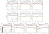 |
Fig. 5. Same as Fig. 3, but for a 0.6 M⊙ (top line), 0.8 M⊙ (middle), and 1.2 M⊙ (bottom) star. |
| In the text | |
|
Fig. 6. Same as Fig. 4, but from left to right: Transmission function, 𝒫m, for the 0.6 M⊙, 0.8 M⊙, and 1.2 M⊙ stellar models along their respective evolution, in the case with rotation and magnetism. |
| In the text | |
Current usage metrics show cumulative count of Article Views (full-text article views including HTML views, PDF and ePub downloads, according to the available data) and Abstracts Views on Vision4Press platform.
Data correspond to usage on the plateform after 2015. The current usage metrics is available 48-96 hours after online publication and is updated daily on week days.
Initial download of the metrics may take a while.