| Issue |
A&A
Volume 708, April 2026
|
|
|---|---|---|
| Article Number | A196 | |
| Number of page(s) | 15 | |
| Section | Extragalactic astronomy | |
| DOI | https://doi.org/10.1051/0004-6361/202555694 | |
| Published online | 08 April 2026 | |
Accurate polarization calibration of FAST spectral data for measurements of Zeeman splittings of OH megamasers in IRAS 02524+2046
1
National Astronomical Observatories, CAS, Jia-20 Datun Road, Chaoyang District, Beijing 100101, PR China
2
School of Astronomy and Space Sciences, University of Chinese Academy of Sciences, Beijing 100049, China
3
State Key Laboratory of Radio Astronomy and Technology, Beijing 100101, China
★ Corresponding author: This email address is being protected from spambots. You need JavaScript enabled to view it.
Received:
28
May
2025
Accepted:
10
February
2026
Abstract
Context. An accurate polarization calibration is essential for a spectral data analysis and Zeeman splitting measurements. Two anomalies challenge our understanding of OH megamasers in IRAS 02524+2046: an unexplained 1667/1665 MHz flux-ratio deviation, and complex Stokes V signatures. Well-calibrated sensitive polarization observations are required to understand them.
Aims. We develop a polarization calibration solution for the L-band 19-beam receiver installed on the Five-hundred-meter aperture spherical radio telescope (FAST) to achieve a high calibration accuracy and thus enable accurate measurements of the OH megamaser properties in IRAS 02524+2046.
Methods. We determined the Mueller matrix solution for spectral observations across the 1050−1450 MHz frequency range with an accuracy of ∼0.01%−0.08% for circular polarization. We then applied it to FAST observational data of IRAS 02524+2046.
Results. Our results show narrower emission line components in the OH megamasers than previously reported, which are indistinguishable in the total power spectrum, but are detected in the circular polarization spectrum. The 1667 MHz OH megamaser emissions probably span a wide velocity range from vhelio ∼ 54 750 to ∼53 580 km s−1, indicating greater complexity than previously recognized. Our fit of the total power and circular polarization spectra for IRAS 02524+2046 revealed ten line components with significant Zeeman splitting (> 3σ), indicating in situ magnetic fields with a strength of approximately −24.5 mG to +20.6 mG, most of which (8/10) have positive values.
Key words: magnetic fields / masers / polarization / ISM: magnetic fields / galaxies: magnetic fields / galaxies: starburst
© The Authors 2026
 Open Access article, published by EDP Sciences, under the terms of the Creative Commons Attribution License (https://creativecommons.org/licenses/by/4.0), which permits unrestricted use, distribution, and reproduction in any medium, provided the original work is properly cited.
This article is published in open access under the Subscribe to Open model. This email address is being protected from spambots. You need JavaScript enabled to view it. to support open access publication.
1. Introduction
An accurate polarization calibration is essential for analyzing spectral radio data. In general, the Mueller matrix for the entire observation system is determined through multiple observations of a standard polarization calibrator (e.g., 3C 286) at various parallactic angles (Heiles et al. 2001; Robishaw 2008; Robishaw & Heiles 2021; Ching et al. 2022, 2025). These polarization observations for an accurate calibration require significant telescope time.
The Five-hundred-meter aperture spherical radio telescope (FAST) is currently the world’s largest single-dish radio telescope (Nan 2006). With its 300 m illuminated aperture and the sensitive L-band 19-beam receiver covering 1000−1500 MHz (Jiang et al. 2020), it possesses exceptional capabilities for observing pulsars (e.g., Han et al. 2021; Zhou et al. 2023b; Xu et al. 2022), fast radio bursts (e.g., Zhou et al. 2023a), radio continuum emission (e.g., Gao et al. 2022), and spectral lines (e.g., Hong et al. 2022; Hou et al. 2022). Since its commissioning in 2019, FAST has conducted multiple observations of polarization calibrators. A circular polarization calibration accuracy on the order of 10−4 for the central beam has been achieved by Ching et al. (2022). Based on observations of the calibrators 3C 286, 3C 48, and 3C 138, Ching et al. (2025) recently characterized the temporal variations of the Mueller matrix elements for the polarization calibration for the 19 beams. An accurate calibration for all beams requires regular observations of polarization calibrators. The currently available observation data from FAST are insufficient for the purpose.
During spectral line observations, the calibration signals are routinely injected into the system in on-off mode for a rapid calibration. This approach enables us to determine gain and phase differences and variations between the receiver’s two linearly polarized channels, as demonstrated in continuum polarization studies (e.g., Gao et al. 2022; Xiao et al. 2023) and pulsar polarization research (e.g., Wang et al. 2023, 2024). Since the commissioning of early scientific observations in 2019, FAST has accumulated a substantial volume of spectral line data using its L-band 19-beam receiver. The spectral backends record all four polarization products (XX, YY, Re[X*Y], and Im[X*Y]) from the radio signals received through the two orthogonal linear polarizations X and Y.
We develop the procedures for accurately calibrating the full-polarization spectral data obtained by FAST. We then apply our approach to observations of OH megamasers in IRAS 02524+2046, which were observed in our projects to validate the data processing pipeline and Stokes V sign convention. The unprecedented sensitivity of FAST reveals new properties of OH megamasers in this galaxy. We briefly introduce the IRAS 02524+2046 and FAST observations in Section 2. The polarization calibration procedures are presented in Section 3. The new results for OH megamasers in IRAS 02524+2046 are presented in Section 4. Our discussions and conclusions are given in Section 5.
2. OH megamasers of IRAS 02524+2046 and FAST observations
The galaxy IRAS 02524+2046 is a starburst galaxy (Peng et al. 2020) and hosts luminous OH megamasers exhibiting unusual line ratios (Darling & Giovanelli 2002a; McBride et al. 2013). The OH spectrum of this galaxy presents broad-line components together with multiple strong and narrow components of the 1667 and 1665 MHz transitions. Some spectral components show day-to-day variation (Darling 2005, 2007). No satellite lines of the OH ground state near the rest frequency of 1612 MHz or 1720 MHz were detected (McBride et al. 2013). Observations with a high spatial resolution reveal that the compact maser emission line sources are distributed across a region of ∼210 × 90 pc (Peng et al. 2020; Wu et al. 2023).
There are two unresolved issues regarding the OH megamasers in IRAS 02524+2046. One issue is the anomalous flux ratio for the pair of the 1667 and 1665 MHz lines (Darling & Giovanelli 2002a; McBride et al. 2013), and the other issue is the complex features in the Stokes V spectrum (McBride & Heiles 2013). The high-velocity feature at vhelio ∼ 54 725 km s−1, attributed to the OH 1665 MHz transition in previous studies (Darling & Giovanelli 2002a; McBride et al. 2013; Peng et al. 2020), shows an unusually strong integrated flux density compared to the 1667 MHz line at a heliocentric velocity vhelio ∼ 54 300 km s−1. Unless otherwise specified, the vhelio of the observed spectrum throughout this work was calculated using the rest frequency ν0 = 1667.3590 MHz. The line ratio RH = F1667/F1665, where Fν represents the integrated flux density across each emission line, is about 1.3 (McBride et al. 2013) or 1.4 (Darling & Giovanelli 2002a), which is in the range of thermal emission values of 1.0 − 1.8. It presents a challenge to the pumping model of OH megamasers (Lockett & Elitzur 2008), which predicts that the 1667 MHz line dominates the 1665 MHz line for line widths exceeding ∼2 km s−1, as commonly seen in OH megamasers. Even after multi-Gaussian decomposition, both lines of the pair of 1667 and 1665 MHz transitions maintain significantly broader line widths (> 2 km s−1). On the other hand, it is difficult to fit the Stokes V spectrum features (McBride & Heiles 2013) to demonstrate the Zeeman splitting and derive the magnetic fields of OH megamasers, because significant residuals with prominent peaks and dips persist in all fitting attempts.
IRAS 02524+2046 was observed by FAST during two observation sessions (see below) using the central beam of the L-band 19-beam receiver with a zenith angle from approximately 24.7° to 9.4° and a small system temperature change in a range of about Tsys ∼ 23 K to 20 K (Jiang et al. 2020). The two linear polarization signals X and Y were extracted by an orthomode transducer for each of the 19 beams, making this system particularly well suited for precise measurements of circular polarization signals (Heiles et al. 2001) (see Table 1).
OH megamaser observation parameters for IRAS 02524+2046.
The first observation was carried out on 11 August 2023 using the central beam of the L-band 19-beam receiver. The TrackingWithAngle mode was adopted to track the target for approximately one hour, with a pointing accuracy of about 8″ (Jiang et al. 2020), a main-beam efficiency of ∼0.63, and a half-power beam width of ∼2.8′ (Jiang et al. 2020) or ∼2.9′ (Chen et al. 2025) at 1420 MHz. During the observations, the receiver continuously rotates to compensate for the real-time field rotation. Additionally, the feed angle can be preset to any value between −80° and +80°. We maintained the default 0° setting of the feed angle for these observations. A calibration signal from a low-noise diode with an amplitude of about 1.1 K (Jiang et al. 2020) was periodically injected for 1 s every 16 s, which can be used to calibrate the temperature scale and the polarization performance of the system (Sun et al. 2021). The polarization signals were recorded across 1024 K channels covering the observing frequencies from 1000 MHz to 1500 MHz, corresponding to a frequency resolution of 0.477 kHz (equivalent to 0.10 km s−1 velocity resolution at the 1420 MHz H I line).
The second observation was conducted on 12 August 2023 using identical instrument settings, but with the feed angle fixed at 45° after compensating for the field rotation to examine potential polarization side-lobe effects. We note that IRAS 02524+2046 is located at Galactic coordinates (l, b) = (158.0°, −33.3°). The spectral line data of the foreground Galactic H I are recorded simultaneously, which provides an independent assessment of the polarization calibration quality, as discussed in subsequent sections.
For the polarization calibration, we obtained five drift-scan observations of the standard calibrator 3C 286 on 19 August 2023 at different rotation angles of −60°, −30°, 0°, +30°, and +60° (e.g., Jiang et al. 2020; Ching et al. 2022, 2025). Given the strong flux density of 3C 286, we employed a high noise diode with an amplitude of about 12.5 K (Jiang et al. 2020) that injected calibration signals in a period of 1 s during the drift scans, with spectral data recorded every 0.5 s. Additionally, we incorporated FAST observations of 3C 286 on 7 and 14 August 2023 using the multi-beam calibration mode during the scheduled maintenance periods to calibrate the flux density.
3. Calibration of polarized spectral data
Based on the intensities of periodically injected reference signals, the four polarization products (XX, YY, Re[X*Y], and Im[X*Y]) were first calibrated to the scale of the antenna temperature TA and were then converted into the heliocentric frame by correcting for the Doppler effect. The radio frequency interference (RFI) in the data was inspected and removed as done by Hou et al. (2022). Afterward, the observed Stokes parameters were derived from the four polarization products using
![Mathematical equation: $$ \begin{aligned} \begin{bmatrix} I_{\rm obs} \\ Q_{\rm obs} \\ U_{\rm obs} \\ V_{\rm obs} \\ \end{bmatrix} = \begin{bmatrix} XX + YY \\ XX - YY \\ 2\mathrm{Re}[X^{*}Y] \\ \pm 2\mathrm{Im}[X^{*}Y] \\ \end{bmatrix}, \end{aligned} $$](/articles/aa/full_html/2026/04/aa55694-25/aa55694-25-eq1.gif) (1)
(1)
where the sign ambiguities in the polarization signals caused by internal cable connections were solved by comparing our results with published values. Following Robishaw et al. (2008) and McBride & Heiles (2013), we adopted the IAU definitions of Stokes V = RCP − LCP, in accordance with the IEEE standard that the right circular polarization (RCP) rotates clockwise as viewed from the radio source, and the left circular polarization (LCP) rotates counterclockwise.
The observed Stokes parameters (Iobs, Qobs, Uobs, and Vobs) are the products of the radio source polarization signals modified by the receiving system of a telescope, as
 (2)
(2)
Here, Mtot is the polarization transfer function of the receiving system (Heiles et al. 2001), which we discuss below. The polarized source signals are modified by the parallactic angle, θ, via
 (3)
(3)
For FAST observations, the feed is always rotated to compensate for field rotation, so this modification is usually not present as θ was set to 0°. To derive intrinsic source properties from the observed Stokes parameters, the polarization transfer function of the receiving system (Heiles et al. 2001), Mtot, has to be solved, which can be expressed as
for the dual linear feeds of the FAST L-band 19-beam receiver (Ching et al. 2025). Here, ϵ denotes the imperfection of the feed in producing nonorthogonal polarizations, ϕ is the phase angle at which the voltage coupling ϵ occurs, α measures the voltage ratio of the polarization ellipse produced when observing a pure linear polarization signal, ΔG indicates the error in the relative intensity calibration of the two polarization channels, and ψ is the phase difference between the reference noise signal and the incoming radiation from the sky,  ,
,  , XQ2Q = −ΔG ϵ cos ϕ sin2α + cos2α, and XQ2U = ΔG ϵ cos ϕ cos2α + sin2α. To determine the intrinsic source properties from the observed Stokes parameters, we investigated two different calibration approaches.
3.1. Polarization calibration resting on injected reference signals
Polarization calibration using the injected reference signals has been successfully applied to various FAST observations, including studies of radio continuum sources and pulsars (e.g., Sun et al. 2021; Wang et al. 2023). Instead of determining all Mueller matrix elements (e.g., Heiles et al. 2001; Robishaw 2008; Robishaw & Heiles 2021), this simplified approach focuses on solving for the two dominant parameters, ΔG and ψ, which account for the mismatch between the amplitudes and phases of the gains of the two orthogonal linear feeds, respectively. This method offers two key advantages. One advantage is that no additional observations of the polarization calibrator are needed, which saves time. The other advantage is that the time-dependent small variation in the system polarization characteristics, even during the observations, can be monitored and corrected.
Following the method of Sun et al. (2021), we determined ΔG and ψ for each frequency channel and applied these corrections to the five 3C 286 drift scans obtained at different rotation angles. We measured a linear polarization fraction  and polarization angle
  at 1400 MHz after ionospheric correction using the ionFR package (Sotomayor-Beltran et al. 2013). These results are roughly consistent with reference values of Psrc = 9.90%±0.003% (Taylor & Legodi 2024) and χ ∼ 27.8° −28.6° at 1400 MHz (Taylor & Legodi 2024) and with our results in Sect. 3.2. According to Ching et al. (2025), the calibrated polarization percentages and polarization angles of 3C 286 measured by FAST at 1420 MHz show Psrc values ranging from ∼9.3% to 9.8% during 2019 to early 2023, with χ values varying between ∼28° and 32°. However, the calibrated V/I values deviate from zero across 1050−1450 MHz, ranging from about −0.5% to +0.4%. The absolute median and mean values are 0.15%±0.01% and 0.17%±0.01%, respectively, indicating that the calibrated V by this method is dominated by the uncompensated leakage of I at the 0.2% level.
To assess the reliability of this simple calibration method, we examined the calibrated spectra of IRAS 02524+2046 around the Galactic H I 21 cm line region. For this target direction, circular polarization of the Galactic H I 21 cm line is expected to be undetectable given our observational integration time. The upper panels of Fig. 1 show that the calibrated V spectrum has a very similar shape as the I profiles near the heliocentric velocity of −10 km s−1, indicating that V has been dominated by the uncompensated leakage of I into V at approximately −0.2% near 1420.4 MHz. For most of the spectra data accumulated by FAST in the past few years, when observational data for determining the full Mueller matrix are lacking and the simple calibration method based on the injected reference signals is applied, the uncompensated leakage of I into V at the ∼0.2% level cannot be corrected.
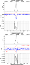 |
Fig. 1. Calibrated results of the Galactic H I 21 cm lines using the two approaches described in Sects. 3.1 and 3.2. These FAST observations targeted IRAS 02524+2046 at Galactic coordinates (l, b) = (158.0°, −33.3°), with a total integration time of 110 minutes. The upper panels demonstrate that the quick calibration method using injected reference signals achieves polarization measurement accuracy of ∼0.2%. The σT lines are derived by considering the contributions from H I emission features following the method of Jing et al. (2023). The lower panels show results after a full Mueller matrix solution and leakage correction, reaching a higher calibration accuracy of ∼0.03%. |
3.2. Polarization calibration based on observations of 3C 286
The standard polarization calibrator 3C 286 was used to determine the Mueller matrix coefficients for the FAST telescope system. In general, the intrinsic circular polarization V of 3C 286 is assumed to be zero at L-band, as confirmed by recent observations (e.g., Taylor & Legodi 2024). To derive the Mueller matrix from FAST’s five 3C 286 drift scans, we implemented the method of Heiles et al. (2001), and we refer to the documentation for the package Robishaw/Heiles SToKes (RHSTK)1 as well as the procedures described in Ching et al. (2025). We fit the observed fractional polarizations (Qobs/Iobs, Uobs/Iobs, and Vobs/Iobs) for each frequency channel. The fitting results for two frequency channels are shown in Fig. 2. Across the frequency ranges of 1050−1150 MHz and 1300−1450 MHz, the fit parameters vary as follows: ΔG, −3.0% to 2.9%; ψ, −0.8° to 1.4°; ϵ, −0.38% to 0.29%; ϕ, 16° to 177°; and α, −0.3° to −0.2° (see Fig. A.1). The Mueller matrix parameters for the 1150−1300 MHz range were not determined due to severe RFI. The derived Mueller matrix was then applied to observational data to obtain corrected Stokes parameters (I, Q, U, V). The sign of Stokes V was verified using previously known results of OH megamasers from IRAS 02524+2046 (McBride & Heiles 2013).
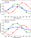 |
Fig. 2. Fitting the observed fractional polarizations in two example frequency channels of 1410 MHz (upper) and 1450 MHz (lower) to derive the Mueller matrix elements. The different symbols indicate different observed fractional polarization components, as shown in the plots. The solid curves show the fitting results. The data were obtained from FAST observations on 19 August 2023. |
Following standard calibration, we measured a linear polarization fraction Psrc = 9.6%±0.3% at 1400 MHz for 3C 286, consistent with the value 9.90%±0.003% given by Taylor & Legodi (2024) and the results of ∼9.3% to 9.8% reported by Ching et al. (2025), and we obtained the polarization angle χ = 36.4° ±0.8°. We calculated the Faraday rotation due to Earth’s ionosphere with the package ionFR (Sotomayor-Beltran et al. 2013), and we then corrected the polarization angle to 27.2° ±0.9° at 1400 MHz, consistent with the intrinsic polarization angle range of about 27.8° −28.6° at 1400 MHz given in Fig. 2 of Taylor & Legodi (2024). This generally agrees with the χ values of ∼28° to 32° at 1420 MHz given by Ching et al. (2025). Across our observed frequency range, the calibrated V/I values are around zero, with absolute median and mean values of 0.03%±0.01% and 0.06%±0.01%, respectively. We understand that the circular polarization of 3C 286 should be zero at L band (e.g., Taylor & Legodi 2024), and any residuals should reflect the uncorrected leakage from I to V (i.e., ανIν) in the calibration procedure above. This interpretation is supported by our subsequent analysis of Galactic H I 21 cm line observations. We then further repaired the leakage terms ανIν by adding them to the calibrated V spectrum, and we achieved a final circular polarization accuracy of about 0.01%−0.08% across 1050 − 1450 MHz.
To verify our calibration results, we analyzed Galactic H I 21 cm line observations toward IRAS 02524+2046 (l = 158.0°, b = −33.3°) obtained with FAST during a 110-minute on-source integration. After the baseline and standing waves were discounted (see Jing et al. 2023, and Appendix B for examples), we derived the Stokes I, V and fractional polarization V/I for the H I 21 cm lines as shown in the lower panels of Fig. 1. The fractional polarization V/I ranges from about −0.06% to 0.06% across the line emission regions. No similar shape of V to the I profiles implies that the uncompensated leakage of I into V, if it exists, will be lower than 0.03% near 1420.4 MHz. These results demonstrate FAST’s capability to measure weak circular polarization with high precision. The consistent V/I levels between calibrated 3C 286 observations and the calibrated Galactic H I 21 cm line observations suggest that the Mueller matrix values for FAST’s central beam probably do not change significantly over timescales of weeks.
For timescales ranging from months to years, the Mueller matrix of FAST’s 19-beam receiver central beam varies in time, as reported by Ching et al. (2025). When applying average Mueller matrix parameters to FAST observations from 2020–2022, fractional circular polarization measurements exceeding 1.5% can be considered reliable detections (Ching et al. 2025). This performance is comparable to the reference-signal calibration method described in Sect. 3.1. These findings, together with our results, highlight the importance of regular calibrator observations for maintaining polarization calibration accuracy.
4. The features of OH megamasers in IRAS 02524+2046 observed by FAST
We applied the Mueller matrix calibration to the IRAS 02524+2046 spectral data and obtained similar results from two independent FAST observations, as shown in Fig. 3. The one-day variation is apparent in some components (Fig. 4). After combining the two datasets, we derived the Stokes I and V spectra of the OH megamasers, as shown in Fig. 5. Because the total on-source integration time is about 110 minutes by the super-sensitive FAST, we obtained the fine spectrum in Fig. 5 with a root mean square (RMS) noise of only about 0.3 mJy per channel at 0.48 km s−1 velocity resolution. Key findings include the detection of detailed OH megamaser features from IRAS 02524+2046 and a high circular polarization reaching up to ∼16% at certain frequencies. As we inspected the raw data in detail, these OH megamaser features detected by FAST are not caused by radio frequency interference.
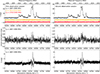 |
Fig. 3. OH megamaser emission from IRAS 02524+2046 observed by FAST during two observation sessions. Top panels: Stokes I spectra aligned by heliocentric velocity for the OH ground-state transitions. The vertical offsets are applied for clarity. Middle panels: Linear polarization spectra for the 1665 MHz and 1667 MHz OH megamaser lines. Bottom panels: Circular polarization spectra for both OH transitions. |
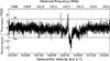 |
Fig. 4. Difference in the Stokes I spectrum between two observation sessions, indicating the one-day variation in the spectral lines. |
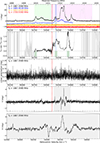 |
Fig. 5. OH megamaser emissions from IRAS 02524+2046 observed by FAST for 110 minutes. Top panel: Stokes I spectra of the OH ground state aligned by heliocentric velocity, with given vertical offsets for clarity. The dashed vertical line marks the heliocentric velocity vhelio = cz = 54 382 km s−1 of IRAS 02524+2046 for a redshift z = 0.1814 from optical spectrophotometry (Darling & Giovanelli 2006). The thick light blue line highlights the pair of 1667 and 1665 MHz OH megamaser lines, showing an unusual flux ratio reported by Darling & Giovanelli (2002a) and McBride et al. (2013). The fuchsia shaded area indicates the probable velocity range of the 1667 MHz OH megamaser emission lines, while the lime shaded area represents the velocity range in which the 1665 and 1667 MHz lines are likely mixed (see Sect. 4.1). Upper middle panel: Intensity ratio of the 1665 MHz to 1667 MHz lines. The dark green shaded areas indicate that the intensity ratio of the 1665 MHz to 1667 MHz transitions is potentially overestimated near vhelio ∼ 54 050 km s−1 and vhelio ∼ 54 300 km s−1, and underestimated near vhelio ∼ 54 725 km s−1. Middle panel: Linear polarization spectrum at the heliocentric velocity for 1667.3590 MHz line. Lower middle panel: Stokes V spectrum at the heliocentric velocity for 1667.3590 MHz line, showing some features from the 1665.4018 MHz transition. Bottom panel: Zoomed-in view of the Stokes V spectral features. |
4.1. The new features of OH megamaser lines
The top panel of Fig. 5 shows the observed Stokes I spectrum against the heliocentric velocity for the two main line transitions of the OH ground state at rest frequencies of 1665.4018 MHz and 1667.3590 MHz and the two satellite lines at the rest frequencies of 1612.2310 MHz and 1720.5300 MHz. The 1612 MHz spectrum shows no detectable features, and the RMS level of ∼0.3 mJy demonstrates FAST’s exceptional sensitivity. A very narrow emission line feature in the 1720 MHz spectrum was detected with a peak flux density of 2.4 ± 0.1 mJy, a line center 54 312.0 ± 0.1 km s−1 in the heliocentric frame, and a full width at half maximum (FWHM) line width 4.6 ± 0.3 km s−1. This feature appears in the two independent FAST observation sessions (see Fig. 3). The line width is smaller than the typical 10 km s−1 width of OH megamaser components (Lockett & Elitzur 2008). To date, OH satellite lines in the L band have only been detected in seven galaxies: Arp 220 (Baan & Haschick 1987; McBride et al. 2013), III ZW 35 (Baan et al. 1989; McBride et al. 2013), IRAS 17207−0014 (Baan et al. 1989; McBride et al. 2013), Arp 299 (IC 694) and Mrk 231 (Baan et al. 1992), IRAS 10173+0829, and IRAS 15107+0724 (McBride et al. 2013).
The dominant 1665 MHz and 1667 MHz OH megamaser features appear within vhelio ∼ 53 800 − 54 850 km s−1, consistent with previous single-dish (Darling & Giovanelli 2002a; McBride et al. 2013; Wu et al. 2023) and interferometry (Peng et al. 2020) observations. However, significant flux density discrepancies exist among different studies. When we take the strongest feature near vhelio ∼ 54 150 km s−1 as an example, the flux density values given by different works are ∼28 mJy (this work), ∼30 mJy (Wu et al. 2023), ∼80 mJy (McBride et al. 2013), and ∼40 mJy (Darling & Giovanelli 2002a). The OH megamaser variability likely contributes to these differences. This variability was first discovered by Darling & Giovanelli (2002b) and is commonly interpreted as a result of interstellar scintillation (e.g., Darling & Giovanelli 2002b; Wu et al. 2023), although not all of the components present apparent variation. Intrinsic changes in the physical conditions of the maser environment (McBride et al. 2015; Harvey-Smith et al. 2016) might also account for the variability. For IRAS 02524+2046, the strong variability of OH megamasers across multiple spectral components has been documented by Arecibo observations. Notably, the RMS spectrum reveals significant day-to-day variations (Darling 2005, 2007). The short-term variability is also evident in our data. As shown in Fig. 4, day-to-day changes are noticeable in some emission components centered from vhelio ∼ 54 000 km s−1 to 54 250 km s−1.
In comparison to previous works, the FAST spectrum presents more detailed emission line features resting on its high sensitivity and high spectral resolution. For instance, a prominent narrow emission line component from the 1667 MHz transition appears near vhelio ∼ 54 327 km s−1, which has a peak flux density of 3.9 ± 0.2 mJy, a line center of 54 326.96 ± 0.06 km s−1, and a FWHM line width of 2.6 ± 0.2 km s−1. The line width is narrower than that of typical OH megamaser components (10 km s−1, Lockett & Elitzur 2008) and is broader than Galactic star-forming region OH masers (≲1 km s−1, e.g., Caswell et al. 2013, 2014). This narrow component is unlikely to originate from RFI, as it was consistently detected across multiple independent observational datasets: in both sessions of our FAST observations, and in the separate observations conducted by Darling & Giovanelli (2002a) and McBride & Heiles (2013) with Arecibo. Outside this velocity range, there are two emission line features. One feature is a new ∼3σ detection at vhelio ∼ 53 580 km s−1, most likely from 1667 MHz OH lines considering its observed frequency. The other is a > 5σ feature at vhelio ∼ 55 140 km s−1, which was previously reported by Darling & Giovanelli (2002a, see the upper right panel of their Fig. 1), and which corresponds to a heliocentric velocity of ∼54 725 km s−1 for 1665 MHz OH transition.
The detection of the 1665 MHz line near the heliocentric velocity of ∼54 725 km s−1 provides crucial insight into the unusual flux ratio of the pair of 1667 MHz and 1665 MHz lines previously reported (Darling & Giovanelli 2002a; McBride et al. 2013). In the Arecibo survey results for 50 OH megamaser galaxies, all the identified 1665 MHz OH megamaser lines showed much stronger 1667 MHz counterparts (Darling & Giovanelli 2000, 2001, 2002a). As shown by the blue spectrum in Fig. 5, the weak feature far left near vhelio ∼ 55 140 km s−1 in the black spectrum should be attributed to the 1665 MHz transition at the heliocentric velocity ∼54 725 km s−1, where a much stronger emission line component appears in the black spectrum. The emission line component near vhelio ∼ 54 725 km s−1 in the black spectrum should not be simply attributed to the 1665 MHz OH megamasers alone, as done by e.g., Darling & Giovanelli (2002a), McBride et al. (2013), and Peng et al. (2020), but is likely to be blended emission from the 1667 MHz and 1665 MHz transitions. We adopted a median RH value of 5.9 and a typical interquartile range of 3.2−8.4 from the OH megamaser sample of Darling & Giovanelli (2002c). Using this typical RH value and the integrated intensity of the 1665 MHz megamasers at vhelio ∼ 55 140 km s−1, we estimated the contribution of the 1667 MHz line to the emission at vhelio ∼ 54 725 km s−1. This allowed us to subsequently estimate an RH value of 2.4 for the emissions near vhelio ∼ 54 300 km s−1. Consequently, the previously reported anomalous line ratio near vhelio ∼ 54 300 km s−1 can be naturally explained by the blending of both lines at the same velocities. Therefore, the intensity ratio of the 1665 MHz to 1667 MHz transitions, shown in the upper middle panel of Fig. 5, is likely overestimated near vhelio ∼ 54 300 km s−1 and underestimated near vhelio ∼ 54 725 km s−1. A potential overestimation may also exist near vhelio ∼ 54 050 km s−1, although the individual maser lines are difficult to distinguish in this region. Our results suggest that the 1667 MHz OH megamaser emission from IRAS 02524+2046 extends beyond vhelio ∼ 54 400 km s−1, with significant components at higher velocities, as shown in Fig. 5. Additionally, we note that the new interpretation reveals that the 1667 MHz OH megamaser emissions are distributed on either side of the systemic velocity of IRAS 02524+2046 (vhelio = 54 382 km s−1, determined from optical spectrophotometry, Darling & Giovanelli 2006). This differs from previous results, which suggested emissions on only one side (e.g., Darling & Giovanelli 2002a; McBride et al. 2013).
The linear polarization spectrum of the 1665 MHz and 1667 MHz OH megamasers is shown in the middle panel of Fig. 5. We detect a polarization feature with ∼3.6σ significance at vhelio ∼ 54 190 km s−1. This feature has a polarized intensity of ∼0.54 mJy compared to the total intensity peak of ∼24 mJy at the same velocity, corresponding to a linear polarization degree of ∼2.3%. The origin of the linear polarization observed in the OH megamasers remains unclear. An instrumental leakage of Stokes I to Q and/or U is unlikely, as the intense OH emission features around vhelio ∼ 54 150 km s−1 in the I spectrum would otherwise also imprint a detectable signature on the linear polarization spectrum. Instead, we speculate that the linear polarization might originate from a π component, a phenomenon detected in approximately 16% of Galactic OH masers, including ground-state and excited-state transitions (Green et al. 2015). No other polarization features with a significance above 3σ are present in the linear polarization spectrum.
The Stokes V spectrum for the main OH ground-state transitions is shown in the lower two panels of Fig. 5. In addition to the three prominent features discussed by McBride et al. (2013), our FAST observations reveal new spectral components that appear as peaks and dips within the velocity range vhelio ∼ 54 070 − 54 350 km s−1. While Zeeman splitting remains the primary mechanism for Stokes V features in OH masers, non-Zeeman effects might contribute as well. Theoretical studies indicated that the linear-to-elliptical polarization conversion and Faraday rotation in maser-emitting clouds can produce antisymmetric V profiles, which particularly affect weakly split interstellar masers of SiO, H2O, and CH3OH (Watson 2009). For OH masers in star-forming regions, observed V profiles typically reflect Zeeman splitting, but might be modified by magnetic field gradients, velocity gradients, and radiative transfer effects (e.g., Nedoluha & Watson 1990). The situation becomes more complex for OH megamasers, where line couplings between Doppler-shifted transitions (e.g., the 1665 MHz and 1667 MHz lines) in the velocity gradient conditions of gas clouds might additionally affect the V profiles, although the observed V profiles of OH megamasers are also thought to be Zeeman dominated (Robishaw et al. 2008; McBride & Heiles 2013). Following established methods (Robishaw et al. 2008; McBride & Heiles 2013), we analyzed the observed Stokes I and V spectra to extract magnetic field information.
4.2. The Zeeman splittings of OH megamaser lines
Following Robishaw et al. (2008) and McBride & Heiles (2013), we assumed that the Zeeman splitting of every OH megamaser component is smaller than the line width. The V spectrum can then be expressed as
 (4)
(4)
where ν is the observing frequency, ν0i is the rest frequency of the OH transition for the ith OH megamaser line component, ν/ν0i accounts for the frequency compression of the redshifted line, Ii is the total intensity profile of the ith OH megamaser component, bi is the splitting coefficient, which is 1.964 Hz μG−1 for the 1667.3590 MHz line and 3.270 Hz μG−1 for the 1665.4018 MHz line (Heiles et al. 1993; Robishaw 2008), and B//i is the strength of the line-of-sight magnetic field with a positive value for magnetic fields pointing away from the observer. The parameter CI2V was originally used to quantify the uncompensated leakage from Stokes I to V. However, in our analysis, the fitted CI2V represents a composite signal, which includes both the genuine uncompensated I-to-V leakage and residual standing wave contamination. This is because residual components persist despite the modeling and subtraction of the broad-scale slope of the standing wave, as illustrated in Appendix B.
As discussed in Sect. 4.1, all the OH emission lines with vhelio ≲ 54 400 km s−1 stem from the 1667 MHz OH megamasers, and we hence adopted bi = 1.964 Hz μG−1 in the fitting. As discussed above, the 1667 and 1665 MHz OH emission lines are likely mixed for the emission feature near vhelio ∼ 54 725 km s−1. For the velocity range vhelio ∼ 54 400 − 54 700 km s−1, the 1667 and 1665 MHz lines might also be mixed, although observational support remains insufficient for two reasons: (1) as shown in the upper panel of Fig. 5, no obvious 1665 MHz emissions are detected in the range vhelio ∼ 54 800 − 55 100 km s−1, and (2) the intensity ratio of the 1665 MHz to 1667 MHz lines in vhelio ∼ 54 100 − 54 200 km s−1 is not anomalous. At least two possibilities exist: (1) the OH emissions in vhelio ∼ 54 400 − 54 700 km s−1 are dominated by the 1665 MHz transition, or (2) these emissions are primarily from the 1667 MHz transition, but lack counterparts of 1665 MHz emissions at similar velocities. Based on the available FAST single-dish data, it remains challenging to distinguish between these scenarios. If the emissions in the velocity range vhelio ∼ 54 400 − 54 725 km s−1 result from a combination of the 1665 MHz and 1667 MHz lines, the magnetic field fitting will involve derivatives of the Stokes I emission with uncertain contributions from each line, leading to a complex error propagation. For simplicity, we first adopted bi = 3.270 Hz μG−1 for OH emission lines with vhelio > 54 400 km s−1, and we then used bi = 1.964 Hz μG−1 to repeat the fitting for further discussion.
In the following, we apply two methods to fit the observed I and V spectra. The first method follows the procedures described by Robishaw et al. (2008) and McBride & Heiles (2013) and first decomposes the I spectrum into multiple Gaussians and then examines the possible Zeeman splittings. The second method is to fit the I and V spectra simultaneously with multiple Gaussian components.
4.2.1. Fitting using the first method
Following the method described by Robishaw (2008) and McBride & Heiles (2013), we began by solving equation (4) by decomposing the Stokes I spectrum into multiple Gaussian components. Using the 18 Gaussian components given by McBride & Heiles (2013) as initial guesses, we identified five additional Gaussian components required to fit the features revealed by FAST observations. These include two emission line components near vhelio ∼ 55 140 km s−1 and ∼53 580 km s−1, one narrow emission line near vhelio ∼ 54 327 km s−1, and two components for resolved peaks around vhelio ∼ 54 180 km s−1 in the Stokes I spectrum. The fitting result of Stokes I is shown in the upper panel of Fig. 6. Then, these Gaussian components were used to derive dI/dν to fit the V spectrum (e.g., Robishaw et al. 2008; McBride & Heiles 2013), as presented in Fig. 6. The corresponding parameters are listed in Table 2.
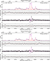 |
Fig. 6. Zeeman-splitting analysis of OH megamaser lines from IRAS 02524+2046. Upper panels: Stokes I and V spectral fits obtained using the method described in Sect. 4.2.1 (fitting method 1), while the lower panels display results from another approach in Sect. 4.2.2 (fitting method 2). For heliocentric velocity calculations, we adopted a rest frequency of ν0 = 1667.3590 MHz, although some spectral features originate from the 1665.4018 MHz OH transition. |
Consistent with McBride & Heiles (2013), we obtained satisfactory fits for the Stokes I spectrum of OH megamasers in IRAS 02524+2046, but encountered difficulties in fitting the complex V profile features. Significant residuals (> 3σT, see Fig. 6) persist in the velocity range vhelio ∼ 54 050 − 54 250 km s−1, despite attempts to optimize initial guesses for a simultaneous I and V spectrum fitting. McBride & Heiles (2013) reported confident magnetic field detections (+12.27 to +23.88 mG) for five narrow components (Gaussians 3, 8, 9, 12, and 13 in their Table 7). We reproduced four of these components, but did not detect their Gaussian component 13 because the local peak at 1412.5320 MHz observed by McBride & Heiles (2013) is absent in our FAST spectra. Our magnetic field measurements agree with theirs within 3σ uncertainties for components 3, 8, and 9 in their Table 7. However, for their component 12 (B// = 13.65 ± 1.07 mG in McBride & Heiles 2013), we measure a smaller field (6.8 ± 0.2 mG, i.e., our component 18 in Table 2). The discrepancy in the fitting results for this component is likely attributable to the intrinsic variability of the magnetic field. Moreover, these findings support a predominantly positive orientation of the magnetic field within the OH megamasers of IRAS 02524+2046.
4.2.2. Fitting using the second method
An optimal decomposition of multiple OH megamaser components should accurately reproduce the I spectrum and detailed V spectrum features. To achieve this, we improved the initial fitting method by simultaneously fitting the I and V spectra with additional Gaussian components, which significantly reduced the residuals present in previous approaches. For model selection, we employed the Akaike information criterion (AIC, Akaike 1974) and Bayesian information criterion (BIC, Schwarz 1978) to balance the goodness-of-fit against the model complexity. The AIC is calculated as Nln(∑(yimodel − yiobs)2/N)+2k, and the BIC = Nln(∑(yimodel − yiobs)2/N)+kln(N), where N represents the number of spectral channels, k is the number of free parameters, and yimodel and yiobs denote the modeled and observed flux densities in the ith channel respectively. These criteria enabled us to fit spectral features above 3σT significance (see Fig. 6) while minimizing the number of Gaussian components required to achieve reasonable residuals.
The lower panel of Fig. 6 shows that the final model incorporates 25 Gaussian components and successfully reproduces the I and V spectra. The corresponding parameters are listed in Table 3. To estimate the parameter uncertainties, we employed a bootstrap resampling approach by separating the IRAS 02524+2046 observational data into 110 files, each of which contained the observational results of one minute on-source integration. We generated 1000 bootstrap samples for the I and V spectra by random resampling. The fitting results of the 1000 samples were used to calculate parameter errors.
Compared to the first method, our analysis reveals two additional Gaussian components in the velocity range vhelio ∼ 54 050 − 54 250 km s−1, corresponding to complex features in the I and V profiles. We detect significant magnetic fields (> 3σ) for ten components: eight components from the 1667 MHz transition, and two components from the assumed 1665 MHz line as given in Table 3. The measured field strengths range from −24.5 mG to +20.6 mG, with a predominance of positive values (8/10 cases). To verify these results, we independently analyzed data from both observational epochs and found consistent magnetic field measurements within 3σ uncertainties, as tabulated in Table 3. For four of the five components with previously reported confident detections by McBride & Heiles (2013, their Gaussians 3, 8, 12, and 13), our measurements agree within 3σ uncertainties. However, we obtained negative field values for the remaining one component, where McBride & Heiles (2013) reported positive fields. Based on earlier findings, the emissions in the velocity range vhelio ∼ 54 400 − 54 725 km s−1 likely represent a blend of the 1665 MHz and 1667 MHz OH lines. We therefore reapplied the fitting procedure by adopting a splitting coefficient bi = 1.964 Hz μG−1. With the exception of Gaussian components 4 and 5, the derived magnetic fields are consistent with the values reported in Table 3. Specifically, the best-fit solutions for components 4 and 5 yield larger magnetic field strengths and associated uncertainties: 6.6 ± 1.3 mG and 12.1 ± 2.8 mG, respectively.
In the fitting results of Stokes V spectra (Fig. 6), the narrow emission line near vhelio ∼ 54 327 km s−1 cannot be well fit by the above methods, warranting further observational investigation. The narrow emission line shows a velocity offset of about 0.5 km s−1 between its Stokes I peak (vhelio ∼ 54 326.96 km s−1) and Stokes V peak (vhelio ∼ 54 326.42 km s−1), with a line width of approximately 2.6 km s−1 in the Stokes I spectrum. One possible explanation is that it corresponds to one component of a Zeeman pair whose LCP and RCP components are split by an interval larger than the line width, and only the stronger component is detected. As observed in Galactic OH masers (e.g., Green et al. 2015), the ratios of the peak flux densities between the LCP and RCP components for Zeeman pairs can range from 0.3 to 2.4.
5. Discussions and conclusions
We developed polarization calibration procedures for L-band spectral observations and applied them to FAST data of the OH megamaser galaxy IRAS 02524+2046. Through complete Mueller matrix solutions, we achieved a circular polarization calibration with an accuracy of ∼0.01%−0.08% across the 1050−1450 MHz frequency range. We also emphasize that regular calibrator observations are necessary to maintain the polarization calibration accuracy.
The FAST observations of IRAS 02524+2046 revealed detailed OH megamaser features in the Stokes I spectrum, including a narrow emission line component with a line width of 2.6 km s−1, two emission line components showing large velocity shifts from the systemic galaxy velocity, and multiple OH emission peaks resolved by the high-spectral resolution. In addition, a narrow emission line feature near the expected frequency of the redshifted 1720 MHz OH line was detected, making IRAS 02524+2046 a new galaxy with a detected OH satellite line.
The detection of the 1665 MHz OH megamaser feature at the heliocentric velocity ∼54 725 km s−1 is particularly significant and suggests that the previously observed unusual flux ratio of the pair of 1665 and 1667 MHz OH megamasers likely results from blended emission of both transitions at similar observed frequencies. Our analysis revealed that the 1667 MHz OH megamaser emission lines in IRAS 02524+2046 spans an exceptionally wide velocity range from vhelio ∼ 54 750 to ∼53 580 km s−1, indicating greater complexity than previously recognized. These observations imply that some maser-emitting clumps exhibit large velocity offsets from the systemic galaxy velocity, which is intriguing for OH megamaser galaxies (e.g., Harvey-Smith et al. 2016). Possible explanations include outflows driven by active galactic nuclei, nuclear starbursts, combined effects of active galactic nuclei and starbursts (e.g., González-Alfonso et al. 2017), an association with dual galactic nuclei, or a molecular ring orbiting a supermassive black hole (e.g., Harvey-Smith et al. 2016).
The sensitive polarization observations by FAST reveal detailed local features in the Stokes V profiles of the 1665 and 1667 MHz OH megamasers from IRAS 02524+2046, including distinct peaks and dips. We simultaneously fit the I and V spectra to decompose the OH megamaser emissions into multiple Gaussian components, identifying ten components with significant Zeeman splitting (> 3σ). The derived magnetic field strengths span −24.5 mG to +20.6 mG, with eight components showing positive values.
The case study of IRAS 02524+2046 demonstrated that sensitive polarization observations with a high spectral resolution are essential for resolving individual maser components and their Zeeman splitting features. These results also indicate that magnetic field measurements derived from some of the individual Gaussian components in single-dish observations require careful interpretation. The overall preferential magnetic field orientation of a galaxy likely provides more reliable physical insight, although high angular resolution very long baseline observations may ultimately be needed to reliably measure the characteristics of the magnetic fields traced by OH megamasers.
Acknowledgments
We thank the anonymous referee for the very careful reading and helpful suggestions. This work is supported by the National SKA Program of China (Grant No. 2022SKA0120103) and the National Natural Science Foundation of China (Grant No. 12588202 and 11933011). XYG and JLH are additionally supported by the International Partnership Program of Chinese Academy of Sciences, Grant No. 114A11KYSB20170044. TH thanks the support from the Youth Innovation Promotion Association CAS. LGH thanks for the helpful discussions with Dr. W.C. Jing for the polarization calibration, and Dr. J. Xu for correcting the influence of the Earth’s ionosphere on the calibration results. This work made use of the data from FAST (Five-hundred-meter Aperture Spherical radio Telescope) (https://cstr.cn/31116.02.FAST). FAST is a Chinese national mega-science facility, operated by the National Astronomical Observatories, Chinese Academy of Sciences.
References
- Akaike, H. 1974, IEEE Trans. Autom. Control, 19, 716 [Google Scholar]
- Baan, W. A., & Haschick, A. D. 1987, ApJ, 318, 139 [Google Scholar]
- Baan, W. A., Haschick, A. D., & Henkel, C. 1989, ApJ, 346, 680 [Google Scholar]
- Baan, W. A., Haschick, A., & Henkel, C. 1992, AJ, 103, 728 [Google Scholar]
- Caswell, J. L., Green, J. A., & Phillips, C. J. 2013, MNRAS, 431, 1180 [NASA ADS] [CrossRef] [Google Scholar]
- Caswell, J. L., Green, J. A., & Phillips, C. J. 2014, MNRAS, 439, 1680 [Google Scholar]
- Chen, X., Ching, T.-C., Li, D., et al. 2025, AJ, 169, 158 [Google Scholar]
- Ching, T. C., Li, D., Heiles, C., et al. 2022, Nature, 601, 49 [NASA ADS] [CrossRef] [Google Scholar]
- Ching, T.-C., Heiles, C., Li, D., et al. 2025, AJ, 170, 116 [Google Scholar]
- Darling, J. 2005, ASP Conf. Ser., 340, 216 [Google Scholar]
- Darling, J. 2007, IAU Symp., 242, 417 [Google Scholar]
- Darling, J., & Giovanelli, R. 2000, AJ, 119, 3003 [NASA ADS] [CrossRef] [Google Scholar]
- Darling, J., & Giovanelli, R. 2001, AJ, 121, 1278 [Google Scholar]
- Darling, J., & Giovanelli, R. 2002a, AJ, 124, 100 [Google Scholar]
- Darling, J., & Giovanelli, R. 2002b, ApJ, 569, L87 [NASA ADS] [CrossRef] [Google Scholar]
- Darling, J., & Giovanelli, R. 2002c, ApJ, 572, 810 [NASA ADS] [CrossRef] [Google Scholar]
- Darling, J., & Giovanelli, R. 2006, AJ, 132, 2596 [NASA ADS] [CrossRef] [Google Scholar]
- Gao, X., Reich, W., Sun, X., et al. 2022, Sci. China Phys. Mech. Astron., 65, 129705 [Google Scholar]
- González-Alfonso, E., Fischer, J., Spoon, H. W. W., et al. 2017, ApJ, 836, 11 [Google Scholar]
- Green, J. A., Caswell, J. L., & McClure-Griffiths, N. M. 2015, MNRAS, 451, 74 [NASA ADS] [CrossRef] [Google Scholar]
- Han, J. L., Wang, C., Wang, P. F., et al. 2021, RAA, 21, 107 [Google Scholar]
- Harvey-Smith, L., Allison, J. R., Green, J. A., et al. 2016, MNRAS, 460, 2180 [NASA ADS] [CrossRef] [Google Scholar]
- Heiles, C., Goodman, A. A., McKee, C. F., & Zweibel, E. G. 1993, in Protostars and Planets III, eds. E. H. Levy, & J. I. Lunine, 279 [Google Scholar]
- Heiles, C., Perillat, P., Nolan, M., et al. 2001, PASP, 113, 1274 [Google Scholar]
- Hong, T., Han, J., Hou, L., et al. 2022, Sci. China Phys. Mech. Astron., 65, 129702 [Google Scholar]
- Hou, L., Han, J., Hong, T., Gao, X., & Wang, C. 2022, Sci. China Phys. Mech. Astron., 65, 129703 [NASA ADS] [Google Scholar]
- Jiang, P., Tang, N.-Y., Hou, L.-G., et al. 2020, RAA, 20, 064 [NASA ADS] [Google Scholar]
- Jing, W. C., Han, J. L., Hong, T., et al. 2023, MNRAS, 523, 4949 [NASA ADS] [CrossRef] [Google Scholar]
- Lockett, P., & Elitzur, M. 2008, ApJ, 677, 985 [Google Scholar]
- McBride, J., & Heiles, C. 2013, ApJ, 763, 8 [NASA ADS] [CrossRef] [Google Scholar]
- McBride, J., Heiles, C., & Elitzur, M. 2013, ApJ, 774, 35 [Google Scholar]
- McBride, J., Robishaw, T., Heiles, C., Bower, G. C., & Sarma, A. P. 2015, MNRAS, 447, 1103 [NASA ADS] [CrossRef] [Google Scholar]
- Nan, R. 2006, Sci. China Phys. Mech. Astron., 49, 129 [Google Scholar]
- Nedoluha, G. E., & Watson, W. D. 1990, ApJ, 361, 653 [Google Scholar]
- Peng, H., Wu, Z., Zhang, B., et al. 2020, A&A, 638, A78 [NASA ADS] [CrossRef] [EDP Sciences] [Google Scholar]
- Robishaw, T. 2008, Ph.D. Thesis, University of California, Berkeley [Google Scholar]
- Robishaw, T., & Heiles, C. 2021, in The WSPC Handbook of Astronomical Instrumentation, Volume 1: Radio Astronomical Instrumentation, ed. A. Wolszczan, 127 [Google Scholar]
- Robishaw, T., Quataert, E., & Heiles, C. 2008, ApJ, 680, 981 [NASA ADS] [CrossRef] [Google Scholar]
- Schwarz, G. 1978, Ann. Stat., 6, 461 [Google Scholar]
- Sotomayor-Beltran, C., Sobey, C., Hessels, J. W. T., et al. 2013, A&A, 552, A58 [NASA ADS] [CrossRef] [EDP Sciences] [Google Scholar]
- Sun, X.-H., Meng, M.-N., Gao, X.-Y., et al. 2021, RAA, 21, 282 [Google Scholar]
- Taylor, A. R., & Legodi, L. S. 2024, AJ, 167, 273 [Google Scholar]
- Wang, P. F., Han, J. L., Xu, J., et al. 2023, RAA, 23, 104002 [NASA ADS] [Google Scholar]
- Wang, T., Wang, C., Han, J. L., et al. 2024, MNRAS, 528, 2501 [Google Scholar]
- Watson, W. D. 2009, Rev. Mexicana Astron. Astrofis. Conf. Ser., 36, 113 [Google Scholar]
- Wu, Z., Sotnikova, Y. V., Zhang, B., et al. 2023, A&A, 669, A148 [NASA ADS] [CrossRef] [EDP Sciences] [Google Scholar]
- Xiao, L., Zhu, M., Sun, X.-H., Jiang, P., & Sun, C. 2023, ApJ, 952, 94 [Google Scholar]
- Xu, J., Han, J., Wang, P., & Yan, Y. 2022, Sci. China Phys. Mech. Astron., 65, 129704 [Google Scholar]
- Zhou, D. J., Han, J. L., Jing, W. C., et al. 2023a, MNRAS, 526, 2657 [Google Scholar]
- Zhou, D. J., Han, J. L., Xu, J., et al. 2023b, RAA, 23, 104001 [Google Scholar]
Appendix A: Parameters of Mueller matrix for the central beam
The fitted values and their associated uncertainties for the five Mueller matrix parameters (ΔG, ψ, ϵ, ϕ, and α) are summarized in the corresponding panels in Fig. A.1 for the 1050−1150 MHz and 1300−1450 MHz frequency bands. As discussed in Ching et al. (2025), the parallactic angle θ and the parameter α are coupled in the solution of the Mueller matrix. A small systematic error in θ may propagate to the fitted α values. In the lower panel of Fig. A.1, the nearly constant fitted α values across different frequencies likely indicate a systematic error in θ originating from imperfections in the mechanical control of the receiver rotation.
Appendix B: Baseline and standing wave removal in spectral data processing
We employ a modified sinusoidal function (Jing et al. 2023) combined with third-order polynomials to model and remove standing waves and spectral baselines. Fig. B.1 and B.2 demonstrate this technique through two applications: (1) Galactic H I 21 cm lines toward IRAS 02524+2046 (Galactic coordinates l = 158.0°, b = −33.3°), and (2) OH megamasers in IRAS 02524+2046.
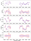 |
Fig. B.1. Frequency dependence of the five fitted Mueller matrix parameters (ΔG, ψ, ϵ, ϕ, and α) across the 1050−1150 MHz and 1300−1450 MHz bands. Data are derived from FAST observations of 3C 286 on 19 August 2023. |
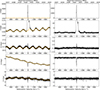 |
Fig. B.2. Left panels show the Stokes I, Q, U, and V spectra (black) of Galactic H I 21 cm emission toward IRAS 02524+2046 (l = 158.0°, b = −33.3°) observed by FAST on 12 August 2023, with orange curves indicating the fitted baseline and standing wave models. The right panels present the spectra after subtracting these components. |
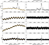 |
Fig. B.3. Same format as Fig. B.1, showing the results for the 1665 MHz and 1667 MHz OH megamaser emission from IRAS 02524+2046 observed by FAST on 12 August 2023. |
All Tables
All Figures
|
Fig. 1. Calibrated results of the Galactic H I 21 cm lines using the two approaches described in Sects. 3.1 and 3.2. These FAST observations targeted IRAS 02524+2046 at Galactic coordinates (l, b) = (158.0°, −33.3°), with a total integration time of 110 minutes. The upper panels demonstrate that the quick calibration method using injected reference signals achieves polarization measurement accuracy of ∼0.2%. The σT lines are derived by considering the contributions from H I emission features following the method of Jing et al. (2023). The lower panels show results after a full Mueller matrix solution and leakage correction, reaching a higher calibration accuracy of ∼0.03%. |
| In the text | |
|
Fig. 2. Fitting the observed fractional polarizations in two example frequency channels of 1410 MHz (upper) and 1450 MHz (lower) to derive the Mueller matrix elements. The different symbols indicate different observed fractional polarization components, as shown in the plots. The solid curves show the fitting results. The data were obtained from FAST observations on 19 August 2023. |
| In the text | |
|
Fig. 3. OH megamaser emission from IRAS 02524+2046 observed by FAST during two observation sessions. Top panels: Stokes I spectra aligned by heliocentric velocity for the OH ground-state transitions. The vertical offsets are applied for clarity. Middle panels: Linear polarization spectra for the 1665 MHz and 1667 MHz OH megamaser lines. Bottom panels: Circular polarization spectra for both OH transitions. |
| In the text | |
|
Fig. 4. Difference in the Stokes I spectrum between two observation sessions, indicating the one-day variation in the spectral lines. |
| In the text | |
|
Fig. 5. OH megamaser emissions from IRAS 02524+2046 observed by FAST for 110 minutes. Top panel: Stokes I spectra of the OH ground state aligned by heliocentric velocity, with given vertical offsets for clarity. The dashed vertical line marks the heliocentric velocity vhelio = cz = 54 382 km s−1 of IRAS 02524+2046 for a redshift z = 0.1814 from optical spectrophotometry (Darling & Giovanelli 2006). The thick light blue line highlights the pair of 1667 and 1665 MHz OH megamaser lines, showing an unusual flux ratio reported by Darling & Giovanelli (2002a) and McBride et al. (2013). The fuchsia shaded area indicates the probable velocity range of the 1667 MHz OH megamaser emission lines, while the lime shaded area represents the velocity range in which the 1665 and 1667 MHz lines are likely mixed (see Sect. 4.1). Upper middle panel: Intensity ratio of the 1665 MHz to 1667 MHz lines. The dark green shaded areas indicate that the intensity ratio of the 1665 MHz to 1667 MHz transitions is potentially overestimated near vhelio ∼ 54 050 km s−1 and vhelio ∼ 54 300 km s−1, and underestimated near vhelio ∼ 54 725 km s−1. Middle panel: Linear polarization spectrum at the heliocentric velocity for 1667.3590 MHz line. Lower middle panel: Stokes V spectrum at the heliocentric velocity for 1667.3590 MHz line, showing some features from the 1665.4018 MHz transition. Bottom panel: Zoomed-in view of the Stokes V spectral features. |
| In the text | |
|
Fig. 6. Zeeman-splitting analysis of OH megamaser lines from IRAS 02524+2046. Upper panels: Stokes I and V spectral fits obtained using the method described in Sect. 4.2.1 (fitting method 1), while the lower panels display results from another approach in Sect. 4.2.2 (fitting method 2). For heliocentric velocity calculations, we adopted a rest frequency of ν0 = 1667.3590 MHz, although some spectral features originate from the 1665.4018 MHz OH transition. |
| In the text | |
|
Fig. B.1. Frequency dependence of the five fitted Mueller matrix parameters (ΔG, ψ, ϵ, ϕ, and α) across the 1050−1150 MHz and 1300−1450 MHz bands. Data are derived from FAST observations of 3C 286 on 19 August 2023. |
| In the text | |
|
Fig. B.2. Left panels show the Stokes I, Q, U, and V spectra (black) of Galactic H I 21 cm emission toward IRAS 02524+2046 (l = 158.0°, b = −33.3°) observed by FAST on 12 August 2023, with orange curves indicating the fitted baseline and standing wave models. The right panels present the spectra after subtracting these components. |
| In the text | |
|
Fig. B.3. Same format as Fig. B.1, showing the results for the 1665 MHz and 1667 MHz OH megamaser emission from IRAS 02524+2046 observed by FAST on 12 August 2023. |
| In the text | |
Current usage metrics show cumulative count of Article Views (full-text article views including HTML views, PDF and ePub downloads, according to the available data) and Abstracts Views on Vision4Press platform.
Data correspond to usage on the plateform after 2015. The current usage metrics is available 48-96 hours after online publication and is updated daily on week days.
Initial download of the metrics may take a while.