| Issue |
A&A
Volume 708, April 2026
|
|
|---|---|---|
| Article Number | L1 | |
| Number of page(s) | 10 | |
| Section | Letters to the Editor | |
| DOI | https://doi.org/10.1051/0004-6361/202558147 | |
| Published online | 25 March 2026 | |
Letter to the Editor
Benchmarking pre-main sequence stellar evolutionary tracks using disk-based dynamical stellar masses
1
Dipartimento di Fisica ‘Aldo Pontremoli’, Università degli Studi di Milano, via G. Celoria 16, I-20133, Milano, Italy
2
European Southern Observatory, Karl-Schwarzschild-Strasse 2, D-85748, Garching bei München, Germany
3
Center for Astrophysics | Harvard & Smithsonian, 60 Garden Street, Cambridge, MA 02138, USA
4
University College Dublin (UCD), Department of Physics, Belfield, Dublin 4, Ireland
5
Joint ALMA Observatory, Avenida Alonso de Córdova 3107, Vitacura, Santiago, Chile
6
Lunar and Planetary Laboratory, the University of Arizona, Tucson, AZ 85721, USA
7
Max Planck Institute for Extraterrestrial Physics, Giessenbachstrasse 1, D-85748, Garching, Germany
8
Max-Planck-Institut fur Astronomie (MPIA), Konigstuhl 17, 69117, Heidelberg, Germany
9
Department of Astronomy, University of Virginia, Charlottesville, VA 22904, USA
10
Institute of Astronomy, University of Cambridge, Madingley Road, Cambridge CB3 0HA, UK
11
Department of Astronomy, University of Michigan, 1085 South University Avenue, Ann Arbor, MI 48109, USA
12
Department of Earth, Atmospheric, and Planetary Sciences, Massachusetts Institute of Technology, Cambridge, MA 02139, USA
13
Univ. Grenoble Alpes, CNRS, IPAG, F-38000, Grenoble, France
14
Academia Sinica Institute of Astronomy and Astrophysics, 11F of Astronomy-Mathematics Building, AS/NTU, No.1, Sec 4, Roosevelt Rd, Taipei 106216, Taiwan
★ Corresponding author: This email address is being protected from spambots. You need JavaScript enabled to view it.
Received:
17
November
2025
Accepted:
3
March
2026
Abstract
Stellar masses are a fundamental property to understand models of pre-main sequence evolution, but their values derived from Hertzsprung–Russell (HR) diagrams are strongly model dependent. We benchmark pre-main sequence stellar evolutionary tracks using stellar masses dynamically estimated by fitting a parametric model to ALMA observations of the 12CO (J = 3 − 2) line transition emitted by the disks orbiting 20 sources in the old (4 − 14 Myr) Upper Scorpius star forming region. We derive stellar masses from HR diagram fitting for ten different stellar evolutionary models, which we then compare with their stellar dynamical masses for comparison in the stellar mass range 0.1 − 1.3 M⊙. Models with a moderate-to-low fraction of cold stellar spots (f = 17%) most accurately reproduce the dynamical stellar masses (100% of the targets agree within ±1σ). While a higher spot coverage (f = 34%) provides similar stellar mass predictions similar to magnetic equipartition models, larger fractions (f ≥ 51%) significantly disagree with dynamical masses. Magnetic equipartition models overestimate stellar masses up to a factor ∼20%, whereas non-magnetic models underestimate them up to ∼12%. For some models, there is evidence that the stellar mass discrepancies are anticorrelated with dynamical stellar masses. When stellar dynamical mass priors are considered in HR diagram fitting, the median age of a single source can change up to ∼25%, while the median ages inferred across different tracks become consistent, with the age scatter decreasing by ≳77%. These results provide strong empirical constraints for testing and developing evolutionary models of pre-main sequence stars.
Key words: stars: general / Hertzsprung-Russell and C-M diagrams / planetary systems / stars: pre-main sequence / stars: protostars / starspots
NASA Hubble Fellowship Program Sagan Fellow.
© The Authors 2026
 Open Access article, published by EDP Sciences, under the terms of the Creative Commons Attribution License (https://creativecommons.org/licenses/by/4.0), which permits unrestricted use, distribution, and reproduction in any medium, provided the original work is properly cited.
This article is published in open access under the Subscribe to Open model. This email address is being protected from spambots. You need JavaScript enabled to view it. to support open access publication.
1. Introduction
Theoretical models of star formation and pre-main sequence (PMS) evolution are fundamental for deriving the physical properties of young stellar objects (YSOs). The positions of YSOs on the Hertzsprung-Russell (HR) diagram provide the main pathway to estimating stellar masses and ages for entire populations. These quantities are central to studies of star and planet formation and the evolution of protoplanetary disks (e.g. Palla & Stahler 2000; Hillenbrand et al. 2008; Hosokawa et al. 2011; Pecaut et al. 2012; Vioque et al. 2022; Manara et al. 2023; Ratzenböck et al. 2023a). Accurate YSO masses are also important on large samples, since several fundamental parameters, such as mass-accretion rate and protoplanetary-disk mass, scale with stellar mass (Muzerolle et al. 2003; Andrews et al. 2013; Ansdell et al. 2017) and are required to derive accretion rates themselves (Hartmann et al. 2016). Ages are particularly difficult to constrain (Soderblom et al. 2014), and, when inferred from evolutionary models, they are strongly model dependent. More accurate ages from theoretical models would enable direct comparisons with other timescale indicators, thereby improving our understanding of the dynamics and physics of the processes involved in star formation (e.g., lithium depletion or cluster expansion, from Franciosini et al. 2022 and Miret-Roig et al. 2024, respectively).
Since the seminal works of Hayashi (1961) and Henyey et al. (1965), PMS models have progressively incorporated a wide range of physical components, including convection, atmospheric evolution, accretion history, rotation, magnetic fields, opacities, and cold stellar spots. Benchmarking these models with independent measurements is needed to improve their physics and define the stellar mass and age ranges where they work best (e.g. Simon et al. 2000, 2017, 2019; Rosenfeld et al. 2012; Guilloteau et al. 2014; Czekala et al. 2016; Yen et al. 2018; Sheehan et al. 2019). In this work we compare stellar masses derived from protoplanetary disk rotation, i.e., “dynamical” masses independent of stellar evolutionary models, with stellar masses predicted by modern PMS evolutionary models using observed effective temperatures and luminosities. Specifically, we tested the models of Baraffe et al. (2015), Feiden (2016) (nonmagnetic and magnetic), PARSEC v2.0 (Nguyen et al. 2022), Siess et al. (2000), and SPOTS (Somers et al. 2020, with different cold photospheric spot coverages). This comparison provides a direct benchmark of their predictive power and the relevance of their underlying physics.
2. Sample
The targets were selected based on the availability of accurate dynamical masses, reliable stellar parameters, and precise Gaia parallaxes (ϖ/σ(ϖ) > 10). The parent sample comprises 37 disks in the Upper Scorpius region from Carpenter et al. (2025), for which Zallio et al. (2026) measured dynamical stellar masses modeling ALMA Band 7 12CO J = 3 − 2 visibilities.
We excluded four disks with poorly constrained rotational profiles and two multiple systems from the sample. We then excluded four sources for which the moderate angular resolution prevented reliable constraints on the height of the CO-emitting layer (the red sources in Fig. 2), together with a cloud-absorbed disk with an inconsistent dynamical mass (M★, dyn ∼ 1.4 M⊙, but spectral type M2). The final sample is composed of 20 sources from the sample above that have well-determined stellar properties, which were derived from broad-band, flux-calibrated medium-resolution spectra (Empey et al., in prep.) derived from VLT/X-Shooter and analyzed with FRAPPE (Claes et al. 2024, based on Manara et al. 2013). These spectra are well-suited for young stars because they allow a better modeling of veiling, extinction, and spectral type for the targets (e.g., Herczeg & Hillenbrand 2014; Manara et al. 2013, 2020, 2023).
3. Derivation of dynamical and evolutionary model-based stellar masses
The 12CO J = 3 − 2 visibility modeling is described in detail in Zallio et al. (2026). In brief, the analysis involved fitting a parametric model to ALMA visibilities using the csalt software1 (Andrews et al., in prep.), and sampling the posterior distribution with emcee (Foreman-Mackey et al. 2013). A key free parameter in these models is the stellar mass, which sets the rotational velocity field of the disk and is thus directly constrained by the data. Since the statistical uncertainties reported from Zallio et al. (2026) are unrealistically small, in Appendix A we describe how we assigned uncertainties to these dynamical stellar mass measurements, denoted M★, dyn.
In addition to these dynamical masses, we derived stellar masses from the HR diagram (M★, HRD) using the effective temperatures (Teff) and stellar luminosities (L★) presented in Empey et al. (in prep.) for different PMS evolutionary models. In particular, we used the evolutionary models presented in Baraffe et al. 2015, the magnetic2 and nonmagnetic tracks presented in Feiden (2016), the PARSEC v2.0 tracks presented in Nguyen et al. (2022), the tracks from Siess et al. (2000), and the stellar SPOTS tracks presented in Somers et al. (2020) with five different cold stellar spots’ fractional coverages of the stellar surface (f = 0%, f = 17%, f = 34%, f = 51%, and f = 85%). To extract stellar masses and ages (together with their uncertainties), we used the python package ysoisochrone developed by Deng et al. (2025), which is based on the IDL code developed by Pascucci et al. (2016) that uses a Bayesian inference approach. The HR grids used in this work are publicly available in the last version of ysoisochrone3. More details and the HR diagrams for each model are presented in Appendix B (see Fig. B.1). In Table D.1, we show the collection of stellar masses used and derived in this work.
4. Comparison of M★, dyn and M★, HRD
In Figs. 1 and 2, we compare the dynamical stellar masses (M★, dyn) with the different evolutionary model-based stellar masses (M★, HRD). The fraction of sources with consistent mass estimates is reported as a percentage (see Fig. 2), providing a quantitative measure of consistency between the dynamical stellar masses and the stellar masses provided by each evolutionary model. In addition to the fraction of sources in agreement, we quantified the typical offset between dynamically derived stellar masses and theoretical track-inferred stellar masses by computing the median mass ratio ⟨R⟩=⟨M★, dyn/M★, HRD⟩ where the median is taken over all sources included in the comparison. This ratio provides a robust, dimensionless measure of systematic differences: ⟨R⟩∼1 indicates that the evolutionary model predictions are consistent with the dynamical masses, while values below or above unity indicate systematic over- or underestimation, respectively (see Figs. 1, 2).
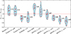 |
Fig. 1. Violin plot of the ratio of the dynamical stellar masses from disk rotation (M★, dyn) and the stellar masses from evolutionary models (M★, HRD) in the 0.1 − 1.3 M⊙ mass range. One-to-one line is indicated with a dashed red line. The median value of M★, dyn/M★, HRD is reported next to each distribution. |
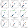 |
Fig. 2. Comparison between dynamical stellar masses, M★, dyn, and the masses from HR-diagram fitting, M★, HRD. The red points represent the excluded sources discussed in Sect. 2, while the orange triangles represent upper and lower mass limits. |
Each pre-main sequence evolutionary model covers a different mass range, as illustrated in the HR diagrams of Fig. B.1. To ensure a fair comparison among the models, we only report the percentage of agreement and the median mass ratio, ⟨R⟩, for sources with a defined mass value in all evolutionary models (i.e., within the mass range of 0.1 < M★ < 1.3 M⊙). We also evaluated the fraction of sources with consistent mass estimates and ⟨R⟩ including upper and lower limits, and found that, apart from minor variations, the results remain unchanged.
5. Results
Figs. 1 and 2 show that the best match with dynamical stellar masses is provided by the SPOTS pre-main sequence tracks with f = 17% cold spot coverage (100% agreement within ±1σ, where σ is the quadratic sum of the model and dynamical mass uncertainties) in the 0.1 − 1.3 M⊙ stellar range. Indeed, several authors (e.g., Grankin et al. 2008; Gully-Santiago et al. 2017; Gangi et al. 2022; Pérez Paolino et al. 2023, 2024) invoked moderate to extreme filling factors (f ∼ 17 − 90%) to model the spectra of Class II sources. Fang & Herczeg (2025) concluded that f ∼ 34 − 51% spot coverage was needed to achieve consistent age estimates across spectral types. We find that f = 17% works better at predicting stellar masses than higher fractional spot coverages. SPOTS models with f = 17% (constant for the entire mass range of considered YSOs) predict stellar masses that are in between the measurements of the Feiden (2016) nonmagnetic and magnetic tracks. When the stellar spot fraction increases (e.g., f = 51%, f = 85%; Fig. 2), the percentage of agreement decreases (33% for f = 51%, and 13% for f = 85%). The SPOTS models with f = 0% behave similarly to the tracks of Baraffe et al. (2015) and Feiden (2016) that are nonmagnetic (see Fig. 1), and they have a percentage of agreement of 87%, similar to that of the Feiden (2016) magnetic tracks.
The nonmagnetic tracks of Baraffe et al. (2015) and Feiden (2016) give almost identical mass measurements, and the same percentage of agreement (93%), though both underestimate the dynamical stellar masses by 15% and 12%, respectively. When considering the Feiden (2016) magnetic tracks, the percentage of agreement decreases slightly to 87%, and the evolutionary model-based stellar masses tend to overestimate the masses derived from disk rotation by up to 20%.
Other works in the literature have compared the Feiden (2016) magnetic and nonmagnetic tracks. For example, Simon et al. (2019) reported that the magnetic tracks of Feiden (2016) work better than the nonmagnetic ones in the stellar range of 0.4 − 1.0 M⊙. Braun et al. (2021) reported instead that the magnetic tracks work better than the nonmagnetic ones in the stellar range of 0.6 − 1.3 M⊙. Moreover, Towner et al. (2025) recently showed that the magnetic tracks of Feiden (2016) work best for stellar masses M★ ≤ 1 M⊙, while the nonmagnetic ones underestimate the dynamical masses by ≳25%. Our findings suggest that, on average, the agreement in the 0.1 − 1.3 M⊙ stellar range is similar among the two; however, on average, the magnetic tracks overestimate the dynamical masses by ∼20%, while the nonmagnetic ones underestimate the former ones by ∼12%.
The evolutionary model-based stellar masses from the PARSEC v2.0 tracks show an agreement of 53% with the masses from disk rotation, which is lower than what is found for other tracks. This result is expected, as the PARSEC v2.0 tracks were first developed for evolved and massive stars, and were then extended toward lower stellar mass values. The tracks of Siess et al. (2000) give an agreement of 80%, which is worse than those of Baraffe et al. (2015) and Feiden (2016), but better than those of PARSEC v2.0, and they underestimate the dynamical stellar masses by ∼26%.
To assess whether the mass discrepancies exhibit a stellar-mass dependence, we computed Spearman rank correlation coefficients between (M★,HRD−M★,dyn)/M★,dyn and M★,dyn. Most models show no statistically significant correlation (p > 0.05), but PARSEC v2.0 and SPOTS models with f ≥ 51% display a negative correlation (Spearman coefficient ρ ≤ −0.77, with p < 10−3), implying a significant mass-dependent bias.
One limitation of our analysis lies in the assumption of purely Keplerian rotation (including the dependence on the disk’s vertical height) within protoplanetary disks. This simplification neglects the impact of pressure gradients and the disk’s self-gravity, which can modify the velocity field. For instance, Andrews et al. (2024) and Longarini et al. (2025) demonstrated that deviations from Keplerian motion induced by pressure support can alter the inferred mass of the central object by as much as 5 − 10%. However, due to the limited angular (0.1 − 0.3″) and spectral (∼480 ms−1) resolution of the data presented in Carpenter et al. (2025), we emphasize that such deviations remain undetectable, and were therefore not considered in the analysis.
In Appendix C, we demonstrate how age estimates can be improved by prior knowledge of dynamical stellar masses. The comparison shown in Fig. C.1 illustrates that incorporating mass priors from the analysis of Zallio et al. (2026) can shift the ages inferred from HR-diagram fitting with the SPOTS f = 17% tracks by approximately 25% when considering single sources, a result consistent with previous findings (e.g., Rosenfeld et al. 2012). In Fig. C.2, we show the distribution of inferred ages for the Upper Scorpius sources from each set of evolutionary tracks considered in this work, reporting the median value and highlighting how the choice of model leads to significantly different median age estimates. Finally, in Fig. C.3, we show that when a prior on the stellar mass is considered for HR-diagram fitting, the median inferred ages across different tracks become much more consistent, and the scatter among different evolutionary tracks decreases from 3.4 Myr to 0.8 Myr, which is an improvement of ≳77%.
6. Conclusions
By comparing accurate measurements of 12CO disk rotation with stellar masses derived from HR diagrams, we conclude with the points listed below:
-
(i)
-
wThe SPOTS evolutionary tracks of Somers et al. (2020) with f = 17% best reproduce (100% agreement within ±1σ uncertainties) the dynamical stellar masses in the 0.1 − 1.3 M⊙ stellar range.
-
(ii)
On average, the HR-diagram masses derived using the magnetic tracks of Feiden (2016), PARSEC v2.0 (Nguyen et al. 2022), and SPOTS (Somers et al. 2020) with f = 34%, 51%, and 85% overestimate the dynamical masses by ∼20%, ∼21%, ∼20%, ∼27%, and ∼32%, respectively. Those provided by the nonmagnetic tracks of Baraffe et al. (2015), Feiden (2016), Siess et al. (2000), and SPOTS with f = 0% underestimate them by ∼15%, ∼12%, ∼26%, and ∼10%, respectively.
-
(iii)
When using stellar dynamical masses as mass priors for HR-diagram fitting, the median inferred ages across different tracks become consistent, and the scatter decreases by ≳77%, while individual ages can vary by up to ∼25%. For our sample, we find a median age of 6.8 Myr, with a scatter of 0.8 Myr across the ten evolutionary tracks considered.
Since evolutionary models are strongly time-dependent, our comparison demonstrates the consistency of disk-based stellar masses with HR-diagram predictions at the age of Upper Scorpius (4 − 14 Myr, Ratzenböck et al. 2023a,b). Whether this agreement holds at different ages remains to be tested, and it will be explored, for example, with the DEC/O Large Program for the younger ages.
Data availability
Table D.1 is available at the CDS via https://cdsarc.cds.unistra.fr/viz-bin/cat/J/A+A/708/L1, and on GitHub4.
Acknowledgments
We thank the anonymous referee for their careful reading of the manuscript and constructive suggestions. L.Z., M.V. and G.R. are grateful to F. Pérez-Paolino and J. Bary for their important suggestions on pms evolutionary tracks, and to C. Pincon and A. Bressan for their feedback on interpreting the age distributions predicted by different evolutionary models. L.Z. and G.R. acknowledge support from the European Union (ERC Starting Grant DiscEvol, project number 101039651), and from Fondazione Cariplo, grant No. 2022-1217. C.F.M. is funded by the European Union (ERC, WANDA, 101039452). Views and opinions expressed are, however, those of the authors only and do not necessarily reflect those of the European Union or the European Research Council. Neither the European Union nor the granting authority can be held responsible for them. T.P.C. was supported by the Heising-Simons Foundation through a 51 Pegasi b Fellowship. Support for C.J.L. was provided by NASA through the NASA Hubble Fellowship grant No. HST-HF2-51535.001-A. This paper acknowledges the usage of ALMA data (project codes 2011.0.00526.S, 2012.1.00688.S, 2013.1.00395.S, 2018.1.00564.S), and VLT/X-Shooter spectra (project codes 097.C-0378, 0101.C-0866, 105.2082.003, 113.26NN.001, 113.26NN.003, 115.27XL.001).
References
- Andrews, S. M., Rosenfeld, K. A., Kraus, A. L., & Wilner, D. J. 2013, ApJ, 771, 129 [Google Scholar]
- Andrews, S. M., Teague, R., Wirth, C. P., Huang, J., & Zhu, Z. 2024, ApJ, 970, 153 [Google Scholar]
- Ansdell, M., Williams, J. P., Manara, C. F., et al. 2017, AJ, 153, 240 [Google Scholar]
- Baraffe, I., Homeier, D., Allard, F., & Chabrier, G. 2015, A&A, 577, A42 [NASA ADS] [CrossRef] [EDP Sciences] [Google Scholar]
- Braun, T. A. M., Yen, H.-W., Koch, P. M., et al. 2021, ApJ, 908, 46 [NASA ADS] [CrossRef] [Google Scholar]
- Carpenter, J. M., Esplin, T. L., Luhman, K. L., Mamajek, E. E., & Andrews, S. M. 2025, ApJ, 978, 117 [Google Scholar]
- Claes, R. A. B., Campbell-White, J., Manara, C. F., et al. 2024, A&A, 690, A122 [NASA ADS] [CrossRef] [EDP Sciences] [Google Scholar]
- Czekala, I., Andrews, S. M., Torres, G., et al. 2016, ApJ, 818, 156 [NASA ADS] [CrossRef] [Google Scholar]
- Deng, D., Vioque, M., Pascucci, I., et al. 2025, ApJ, 989, 3 [Google Scholar]
- Fang, M., & Herczeg, G. J. 2025, ApJ, 994, 248 [Google Scholar]
- Feiden, G. A. 2016, A&A, 593, A99 [NASA ADS] [CrossRef] [EDP Sciences] [Google Scholar]
- Foreman-Mackey, D., Hogg, D. W., Lang, D., & Goodman, J. 2013, PASP, 125, 306 [Google Scholar]
- Franciosini, E., Tognelli, E., Degl’Innocenti, S., et al. 2022, A&A, 659, A85 [NASA ADS] [CrossRef] [EDP Sciences] [Google Scholar]
- Gangi, M., Antoniucci, S.,Biazzo, K., et al. 2022, A&A, 667, A124 [NASA ADS] [CrossRef] [EDP Sciences] [Google Scholar]
- Grankin, K. N., Bouvier, J., Herbst, W., & Melnikov, S. Y. 2008, A&A, 479, 827 [NASA ADS] [CrossRef] [EDP Sciences] [Google Scholar]
- Guilloteau, S., Simon, M., Piétu, V., et al. 2014, A&A, 567, A117 [NASA ADS] [CrossRef] [EDP Sciences] [Google Scholar]
- Gully-Santiago, M. A., Herczeg, G. J., Czekala, I., et al. 2017, ApJ, 836, 200 [NASA ADS] [CrossRef] [Google Scholar]
- Hartmann, L. 1998, Accretion Processes in Star Formation (Cambridge University Press), 32 [Google Scholar]
- Hartmann, L., Herczeg, G., & Calvet, N. 2016, ARA&A, 54, 135 [Google Scholar]
- Hayashi, C. 1961, PASJ, 13, 450 [NASA ADS] [Google Scholar]
- Henyey, L., Vardya, M. S., & Bodenheimer, P. 1965, ApJ, 142, 841 [Google Scholar]
- Herczeg, G. J., & Hillenbrand, L. A. 2014, ApJ, 786, 97 [Google Scholar]
- Hillenbrand, L. A., Bauermeister, A., & White, R. J. 2008, ASP Conf. Ser., 384, 200 [Google Scholar]
- Hosokawa, T., Offner, S. S. R., & Krumholz, M. R. 2011, ApJ, 738, 140 [NASA ADS] [CrossRef] [Google Scholar]
- Longarini, C., Lodato, G., Rosotti, G., et al. 2025, ApJ, 984, L17 [Google Scholar]
- Manara, C. F., Testi, L., Rigliaco, E., et al. 2013, A&A, 551, A107 [NASA ADS] [CrossRef] [EDP Sciences] [Google Scholar]
- Manara, C. F., Natta, A., Rosotti, G. P., et al. 2020, A&A, 639, A58 [NASA ADS] [CrossRef] [EDP Sciences] [Google Scholar]
- Manara, C. F., Ansdell, M., Rosotti, G. P., et al. 2023, ASP Conf. Ser., 534, 539 [NASA ADS] [Google Scholar]
- Miret-Roig, N., Alves, J., Barrado, D., et al. 2024, Nat. Astron., 8, 216 [Google Scholar]
- Muzerolle, J., Hillenbrand, L., Calvet, N., Briceño, C., & Hartmann, L. 2003, ApJ, 592, 266 [NASA ADS] [CrossRef] [Google Scholar]
- Nguyen, C. T., Costa, G., Girardi, L., et al. 2022, A&A, 665, A126 [NASA ADS] [CrossRef] [EDP Sciences] [Google Scholar]
- Palla, F., & Stahler, S. W. 2000, ApJ, 540, 255 [NASA ADS] [CrossRef] [Google Scholar]
- Pascucci, I., Testi, L., Herczeg, G. J., et al. 2016, ApJ, 831, 125 [Google Scholar]
- Pecaut, M. J., Mamajek, E. E., & Bubar, E. J. 2012, ApJ, 746, 154 [Google Scholar]
- Pérez Paolino, F., Bary, J. S., Petersen, M. S., et al. 2023, ApJ, 946, 10 [Google Scholar]
- Pérez Paolino, F., Bary, J. S., Hillenbrand, L. A., & Markham, M. 2024, ApJ, 967, 45 [CrossRef] [Google Scholar]
- Pinte, C., Ménard, F., Duchêne, G., & Bastien, P. 2006, A&A, 459, 797 [NASA ADS] [CrossRef] [EDP Sciences] [Google Scholar]
- Pinte, C., Harries, T. J., Min, M., et al. 2009, A&A, 498, 967 [NASA ADS] [CrossRef] [EDP Sciences] [Google Scholar]
- Ratzenböck, S., Großschedl, J. E., Alves, J., et al. 2023a, A&A, 678, A71 [NASA ADS] [CrossRef] [EDP Sciences] [Google Scholar]
- Ratzenböck, S., Großschedl, J. E., Möller, T., et al. 2023b, A&A, 677, A59 [NASA ADS] [CrossRef] [EDP Sciences] [Google Scholar]
- Rosenfeld, K. A., Andrews, S. M., Wilner, D. J., & Stempels, H. C. 2012, ApJ, 759, 119 [NASA ADS] [CrossRef] [Google Scholar]
- Sheehan, P. D., Wu, Y.-L., Eisner, J. A., & Tobin, J. J. 2019, ApJ, 874, 136 [NASA ADS] [CrossRef] [Google Scholar]
- Siess, L., Dufour, E., & Forestini, M. 2000, A&A, 358, 593 [Google Scholar]
- Simon, M., Dutrey, A., & Guilloteau, S. 2000, ApJ, 545, 1034 [NASA ADS] [CrossRef] [Google Scholar]
- Simon, M., Guilloteau, S., Di Folco, E., et al. 2017, ApJ, 844, 158 [Google Scholar]
- Simon, M., Guilloteau, S., Beck, T. L., et al. 2019, ApJ, 884, 42 [NASA ADS] [CrossRef] [Google Scholar]
- Soderblom, D. R., Hillenbrand, L. A., Jeffries, R. D., Mamajek, E. E., & Naylor, T. 2014, in Protostars and Planets VI, eds. H. Beuther, R. S. Klessen, C. P. Dullemond, & T. Henning, 219 [Google Scholar]
- Somers, G., Cao, L., & Pinsonneault, M. H. 2020, ApJ, 891, 29 [Google Scholar]
- Towner, A. P. M., Eisner, J. A., Sheehan, P. D., Hillenbrand, L. A., & Wu, Y.-L. 2025, ApJ, 994, 214 [Google Scholar]
- Vioque, M., Oudmaijer, R. D., Wichittanakom, C., et al. 2022, ApJ, 930, 39 [NASA ADS] [CrossRef] [Google Scholar]
- Waskom, M. L. 2021, J. Open Source Softw., 6, 3021 [CrossRef] [Google Scholar]
- Yen, H.-W., Koch, P. M., Manara, C. F., Miotello, A., & Testi, L. 2018, A&A, 616, A100 [NASA ADS] [CrossRef] [EDP Sciences] [Google Scholar]
- Zallio, L., Rosotti, G. P., Vioque, M., et al. 2026, A&A, 705, A49 [NASA ADS] [CrossRef] [EDP Sciences] [Google Scholar]
As reported by the author on the GitHub page, the magnetic tracks available at https://github.com/gfeiden/MagneticUpperSco are incorrect for ages of ≤1 Myr, which contain numerical artifacts; we corrected these by interpolating the data and removing the outliers.
https://github.com/DingshanDeng/ysoisochrone; the specific version (v1.3.3) used in this work is archived on Zenodo at https://zenodo.org/records/18420752
We consider the radius that encompasses 90% of the disk total flux R90% as the gas disk radius.
The Kernel Density Estimation (KDE) is a non-parametric method used to estimate the probability density function (PDF) of a continuous variable from a finite sample.
The Kelvin-Helmholtz timescale is the time over which a star radiates away its gravitational potential energy at its current luminosity: τKH ∼ GM★2/R★L★, where G is the gravitational constant, M★ the mass of the star, R★ its radius and L★ its luminosity.
Appendix A: Uncertainties on the dynamical mass measurements due to inclination, stellar mass, and disk size
Since the stellar mass statistical uncertainties reported by Zallio et al. (2026) are systematically underestimated due to limitations of fitting visibilities with parametric models, we decide to test the accuracy of the csalt dynamical mass measurements by creating and fitting a grid of numerical simulations. After creating mcfost5 (Pinte et al. 2006, 2009) radiative transfer models of 12CO J = 3 − 2, we use built-in routines of csalt to transform them into radio-interferometric observed data, using the same total integration time (∼180 s per disk), S/N, and antenna configurations of the observations analyzed in Zallio et al. (2026), from the sample of Carpenter et al. 2025). Our grid of models tests the accuracy of mass inferences for stars with masses of 1, 0.5, and 0.05 M⊙ to explore stellar mass values down to the sub-stellar range, with disks inclined at 8°, 30°, and 55°. We perform these simulations using a gas disk mass of 10−2 M★, a dust disk mass of 10−4 M★, and three different cut-off radii (Rc = 5, 20, 50 au), mimicking unresolved (less than 3 resolution elements in the diameter), resolved (between 3 and 5 resolution elements in the diameter), and extended (more than 5 resolution elements in the disk diameter) protoplanetary disk extension. These three cases correspond to a disk size6R90% < 50 au, 50 ≲ R90% ≲ 90 au, and R90% > 90 au for the observations studied in Zallio et al. (2026). We then perform fits using csalt with the parametric prescription A (see Zallio et al. 2026; this is a complete disk prescription, which also considers for the emitting height of the optically thick 12CO layer) on the synthetic observation we created. Most of our fits return results in agreement with the true stellar mass, except for the sources with inc = 55°, as shown in Fig. A.1, where the discrepancy is ∼10% in the worst case.
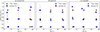 |
Fig. A.1. Results of the fit to unresolved (a), resolved (b), and extended (c) mcfost simulations. The uncertainties on top of the ‘True values’ are the mean of the statistical uncertainties returned by the fit for each mass bin and for each disk size bin, and we plot them for illustrative purposes. |
We use the statistical uncertainties returned by our fits per specific stellar mass range to assign mass uncertainties to the stellar dynamical masses reported in Zallio et al. (2026). We evaluate the mean statistical uncertainty for each stellar bin and for each disk size (reported in the third column of Table A.1) of the uncertainties returned from the csalt fits. This choice is motivated by the fact that the mean statistical uncertainties are found to be greater than the systematic uncertainty, and we therefore opt for a conservative approach. Then, we assign these uncertainties to our observations, as illustrated in Table A.1, using the disk sizes reported in Zallio et al. (2026).
Logic used to assign the uncertainties to the dynamical stellar masses.
Appendix B: HR diagrams
In Fig. B.1, we show the HR diagrams connected to the different evolutionary tracks used in this work. Since each model has a different validity based on different stellar ranges, some sources are found to fall outside (or very close to the edges of) the tracks. In these cases, it is not possible to derive masses and ages from HR diagram fitting using ysoisochrone. We highlight in orange the sources for which it was impossible to derive mass and age, while we show in red the five sources we exclude from the analysis, as reported in Sect. 2. The stellar masses are listed in Table D.1.
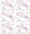 |
Fig. B.1. Hertzsprung–Russell diagrams with the different theoretical evolutionary tracks, the isochrones, and the 25 YSOs considered in this work. |
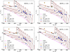 |
Fig. B.2. Continues from Fig. B.1 Hertzsprung–Russell diagrams with the different theoretical evolutionary tracks, the isochrones, and the 25 YSOs considered in this work. |
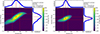 |
Fig. B.3. Example of age determination improvement by using dynamical stellar mass priors, using J16395577-2347355 as an example. On the left, we show the HR diagram best-fit posteriors of age (top panel) and mass (right panel). On the right, we show the distributions obtained after including a gaussian prior on the stellar mass built on the dynamical measure presented in Zallio et al. (2026). The red dot represents the peak of both the mass and age likelihoods. |
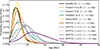 |
Fig. B.4. Different age distributions associated with different evolutionary tracks for the 20 Upper Scorpius sources considered for the comparison. The legend shows the median ages associated to each distribution. |
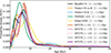 |
Fig. B.5. Different age distributions associated with different evolutionary tracks for the 20 Upper Scorpius sources considered for the comparison after fitting the single HR diagrams using mass priors coming from the stellar dynamical masses. The legend shows the median ages associated to each distribution. |
Appendix C: Stellar ages and the consequences of a prior on the stellar mass
C.1. The impact of stellar mass priors on the age of single objects
Using ysoisochrone, we test how providing a prior on the stellar mass changes the results of HR diagram fitting (following what was done previously in the literature, e.g. Rosenfeld et al. 2012). In Fig. C.1 (left), we show the result of HR diagram fitting using the SPOTS f = 17% tracks (Somers et al. 2020) on one of the sources of our sample: the posterior distribution of age and mass is quite wide.
When including a gaussian mass prior based on the dynamical mass and its associated uncertainty, the age-mass degeneracy reduces greatly, as shown in Fig. C.1 (right). In the case of J16395577-2347355 (one of the most discrepant sources when considering SPOTS f = 17%) we show that the inferred median age changes by ∼25%. When extending this analysis to the whole sample considered with SPOTS f = 17%, the median age changes from 6.3 to 7 Myr, as further shown in Figs. C.2, C.3.
C.2. Age distributions for different evolutionary tracks
In Fig. C.2, we present the age distributions derived from the HR diagram fits performed with ysoisochrone, without applying any mass priors. These distributions are based on the posterior ages obtained for each source. The visualization was produced using the seaborn package (Waskom 2021), which implements Kernel Density Estimation (KDE)7 to provide a smooth representation of the underlying probability density. The resulting distributions show substantial differences among the ten evolutionary models considered. The median age across the models is ∼6.5 Myr, with a scatter of ∼3.4 Myr.
Figure C.3 displays the corresponding age distributions obtained after including priors on the stellar dynamical masses. When the mass prior is introduced, the differences among the distributions become notably smaller. The median age across the ten evolutionary tracks increases slightly to ∼6.8 Myr, while the scatter between the tracks decreases to ∼0.8 Myr.
This result can be explained as follows. The dominant timescale for pre-main sequence stars is the Kelvin-Helmholtz timescale8, since the nuclear fusion has not started yet (see e.g., Hartmann 1998). The stellar radius is fixed by knowing both Teff and L★, thus when we consider a prior on the stellar masses, we force the ages to converge to a fixed value.
Appendix D: Main table with stellar masses
In Table D.1 we show the stellar masses derived for this work for different evolutionary tracks. The disk-based dynamical stellar masses are reported from Zallio et al. (2026).
Stellar masses considered in this work.
All Tables
All Figures
|
Fig. 1. Violin plot of the ratio of the dynamical stellar masses from disk rotation (M★, dyn) and the stellar masses from evolutionary models (M★, HRD) in the 0.1 − 1.3 M⊙ mass range. One-to-one line is indicated with a dashed red line. The median value of M★, dyn/M★, HRD is reported next to each distribution. |
| In the text | |
|
Fig. 2. Comparison between dynamical stellar masses, M★, dyn, and the masses from HR-diagram fitting, M★, HRD. The red points represent the excluded sources discussed in Sect. 2, while the orange triangles represent upper and lower mass limits. |
| In the text | |
|
Fig. A.1. Results of the fit to unresolved (a), resolved (b), and extended (c) mcfost simulations. The uncertainties on top of the ‘True values’ are the mean of the statistical uncertainties returned by the fit for each mass bin and for each disk size bin, and we plot them for illustrative purposes. |
| In the text | |
|
Fig. B.1. Hertzsprung–Russell diagrams with the different theoretical evolutionary tracks, the isochrones, and the 25 YSOs considered in this work. |
| In the text | |
|
Fig. B.2. Continues from Fig. B.1 Hertzsprung–Russell diagrams with the different theoretical evolutionary tracks, the isochrones, and the 25 YSOs considered in this work. |
| In the text | |
|
Fig. B.3. Example of age determination improvement by using dynamical stellar mass priors, using J16395577-2347355 as an example. On the left, we show the HR diagram best-fit posteriors of age (top panel) and mass (right panel). On the right, we show the distributions obtained after including a gaussian prior on the stellar mass built on the dynamical measure presented in Zallio et al. (2026). The red dot represents the peak of both the mass and age likelihoods. |
| In the text | |
|
Fig. B.4. Different age distributions associated with different evolutionary tracks for the 20 Upper Scorpius sources considered for the comparison. The legend shows the median ages associated to each distribution. |
| In the text | |
|
Fig. B.5. Different age distributions associated with different evolutionary tracks for the 20 Upper Scorpius sources considered for the comparison after fitting the single HR diagrams using mass priors coming from the stellar dynamical masses. The legend shows the median ages associated to each distribution. |
| In the text | |
Current usage metrics show cumulative count of Article Views (full-text article views including HTML views, PDF and ePub downloads, according to the available data) and Abstracts Views on Vision4Press platform.
Data correspond to usage on the plateform after 2015. The current usage metrics is available 48-96 hours after online publication and is updated daily on week days.
Initial download of the metrics may take a while.