| Issue |
A&A
Volume 708, April 2026
|
|
|---|---|---|
| Article Number | A130 | |
| Number of page(s) | 12 | |
| Section | Stellar structure and evolution | |
| DOI | https://doi.org/10.1051/0004-6361/202558352 | |
| Published online | 01 April 2026 | |
A highly ionised outflow in the X-ray binary 4U 1624–49 detected with XRISM
1
ESO, Karl-Schwarzschild-Strasse 2, 85748, Garching bei München, Germany
2
SRON Space Research Organisation Netherlands, Niels Bohrweg 4, NL-2333, CA Leiden, The Netherlands
3
Institute of Space and Astronautical Science (ISAS), Japan Aerospace Exploration Agency (JAXA), Kanagawa, 252-5210, Japan
4
Faculty of Science and Technology, Tokyo University of Science, Chiba, 278-8510, Japan
5
Department of Physics, Ehime University, Ehime, 790-8577, Japan
6
Villanova University, Department of Physics, Villanova, PA, 19085, USA
7
NASA/Goddard Space Flight Center, Greenbelt, MD, 20771, USA
8
Center for Research and Exploration in Space Science and Technology, NASA/GSFC (CRESST II), Greenbelt, MD, 20771, USA
9
Center for Space Science and Technology, University of Maryland, Baltimore County (UMBC), 1000 Hilltop Circle, Baltimore, MD, 21250, USA
10
Department of Astronomy, University of Michigan, MI, 48109, USA
11
Anton Pannekoek Institute/GRAPPA, University of Amsterdam, Science Park 904, 1098, XH Amsterdam, The Netherlands
★ Corresponding author: This email address is being protected from spambots. You need JavaScript enabled to view it.
Received:
2
December
2025
Accepted:
22
January
2026
Abstract
Context. The origin of accretion-disc winds remains disputed. High-inclination, dipping, neutron-star (NS) low-mass X-ray binaries (LMXBs) provide an excellent testbed for studying the launching mechanism of such winds due to them persistently accreting and showing a nearly ubiquitous presence of highly ionised plasmas.
Aims. We aim to establish or rule out the presence of a wind in the high-inclination LMXB 4U 1624−49, for which a highly ionised plasma has been repeatedly observed in X-ray spectra by Chandra and XMM-Newton, and a thermal–radiative pressure wind is expected.
Methods. We leveraged the exquisite spectral resolution of the X-ray Imaging and Spectroscopy Mission (XRISM) to perform phase-resolved spectroscopy of the full binary orbit to characterise the highly ionised plasma at all phases except during absorption dips.
Results. An outflow is clearly detected via phase-resolved spectroscopy of the source with XRISM Resolve. Based on analysis of the radial-velocity curve, we determine an average velocity of ∼200−320 km s−1 and a column density above 1023 cm−2. The line profiles are generally narrow, spanning ∼50−100 km s−1, depending on the orbital phase; this points to a low-velocity sheer or turbulence of the highly ionised outflow and a potential increase of turbulence as the absorption dip is approached, likely due to turbulent mixing.
Conclusions. The line profiles, together with the derived launching radius and wind velocity, are consistent with a wind being launched from the outskirts of the disc and without stratification, pointing to a thermal-radiative pressure origin.
Key words: accretion / accretion disks / stars: neutron / X-rays: binaries / X-rays: individuals: 4U 1624–49
© The Authors 2026
 Open Access article, published by EDP Sciences, under the terms of the Creative Commons Attribution License (https://creativecommons.org/licenses/by/4.0), which permits unrestricted use, distribution, and reproduction in any medium, provided the original work is properly cited.
This article is published in open access under the Subscribe to Open model. This email address is being protected from spambots. You need JavaScript enabled to view it. to support open access publication.
1. Introduction
In the past two decades we have witnessed an enormous development in the studies of accretion-disc winds in X-ray binaries. X-ray observations have shown the presence of highly photoionised material, revealed via absorption lines from Fe XXV and Fe XXVI, in the spectra of sources at high inclination (Boirin et al. 2005; Díaz Trigo et al. 2006; Ponti et al. 2012). Significant blueshifts have been measured in a fraction of these systems, indicating outflowing material. While the outflow velocities are moderate, ∼300−3000 km s−1 (Muñoz-Darias et al. 2026), resulting in a modest kinetic-energy output, the estimated mass-outflow rates are of the order of the mass being accreted from the companion, making winds a key ingredient in the accretion process (Ponti et al. 2012; Fender & Muñoz-Darias 2016).
An important step towards understanding the effect of winds in the accretion process and their feedback to the environment is the determining of the wind-launching mechanism. Winds can be launched via thermal, radiative, or magnetic pressure, but the dominant mechanism is still disputed. A fundamental prediction of thermal pressure winds is that they can only be launched at a radius larger than 0.1 of the Compton radius (RIC), where RIC is the radius at which the free-fall velocity equals the isothermal sound speed of the Compton-heated gas (Begelman et al. 1983). The Compton radius is defined as RIC = (1010/TIC, 8)(M/M⊙) cm, where TIC, 8 = TIC/108 and TIC is uniquely dependent on the shape of the spectrum. For X-ray binaries with a soft spectrum, the Compton temperature is 107 K, resulting in RIC ∼ 1011 cm for a NS of 1.4 M⊙. It follows that the velocity should be moderate, of the order of a few hundred km s−1, which is consistent with the escape velocity at such large radii. This and the fact that the flux density of the wind peaks after it is launched (Woods et al. 1996; Tomaru et al. 2020) also makes lines from thermal winds relatively narrow in the absence of additional turbulence since winds are launched across a very narrow range of radii.
In contrast, winds launched by magnetic pressure are expected to be launched throughout the disc, resulting in wider lines and higher velocities (e.g. Fukumura et al. 2017). Moreover, the lack of restriction on the launching radius implies that the capability to launch a wind does not depend on the size of the system.
So far, winds have been found to be launched at relatively large radii and only in systems for which the Compton radius lies inside the disc (Díaz Trigo & Boirin 2016), which is consistent with predictions of thermal winds. However, magnetic winds have also been invoked to explain some wind observations such as the optically thick wind of the black hole LMXB GRO J1655−40 (e.g. Miller et al. 2006) or the variability of such wind following changes in source luminosity or spectral hardness (Neilsen & Homan 2012). Occasionally, spectra with strong absorption features from disc atmospheres show additional weaker features with relatively large blueshifts that have been interpreted as potential evidence of magnetic winds (Trueba et al. 2020).
Studying winds in NS X-ray binaries has the advantage that they generally have a known orbital period and inclination. As such, phase-resolved analyses can, for example, separate the contribution from the wind from absorption from other structures in the disc such as the bulge resulting from the impact of the accretion stream onto the disc.
In this work, we leveraged our knowledge of the high-inclination NS X-ray binary 4U 1624−49 in terms of distance, orbital period, and inclination, with the new capabilities of XRISM (Tashiro et al. 2025). Launched in September 2023, XRISM includes an onboard microcalorimeter called Resolve, which provides spectra in the 1.7−12 keV range (see XRISM Proposers’ Observatory Guide) with a resolution of ∼4.5 eV (FWHM at 5.9 keV, Porter et al. 2025), and a CCD camera called Xtend, which provides moderate-resolution spectroscopy in the 0.4−13 keV energy range over a large region. In particular, the high-resolution microcalorimeter Resolve is crucial to advancing our knowledge of the launching mechanism of winds and testing the prediction that 4U 1624−49 should be able to launch a wind via thermal pressure.
The NS LMXB 4U 1624−49 has a period of 20.87 hours (Smale et al. 2001) and an inclination of 60−75°, derived from the presence of absorption dips on its light curve, which are observed at the orbital period of the system, and the lack of eclipses. A distance of ∼15 kpc was estimated from studies of its dust-scattering halo (Xiang et al. 2009). The companion of 4U 1624−49 was identified as a faint, Ks = 18.3 ± 0.1 infrared source (Wachter et al. 2005), but the high extinction towards the source prevented further characterisation.
Parmar et al. (2002) reported the presence of narrow absorption lines from highly ionised Fe based on XMM-Newton observations for the first time. Díaz Trigo et al. (2006) modelled such lines with photoionised absorbers and found that spectral changes during absorption dips could be explained with an increase of the column density of cold plasma and a decrease of ionisation of the photoionised component. Xiang et al. (2009) extended the work from Parmar et al. (2002) by performing phase-resolved analyses of Chandra observations. They concluded that the absorption was caused by two components: one that is highly ionised and central, consistent with an accretion disc corona (ADC) of radius 3 × 1010 cm, and another less ionised one with its ionisation parameter, ξ, depending on the orbital phase and consistent with it being present at the disc rim at ∼1.1 × 1011 cm. The line widths could be explained by thermal broadening, without significant turbulence or bulk motion needed. They also reported on a sinusoidal modulation of the flux at the orbital period, which they attributed to local cold obscuration rather than intrinsic variability of the source.
Finally, 4U 1624−49 has also been observed by the Imaging X-ray Polarimetry Explorer (IXPE). Gnarini et al. (2024) reported a level of polarisation of 2.7 ± 0.8% during ‘persistent’ emission, the highest of all NS LMXBs with a moderate luminosity (the so-called atoll sources), which they attributed to the Comptonised emission visible in hard X-rays and the high inclination of the system.
2. Observations and data reduction
2.1. XRISM
4U 1624−49 was observed twice with a four-day spacing during the performance-verification (PV) phase of XRISM (see Table 1). The observations were planned to start at the beginning of the dipping phase so that each observation includes one full orbital period plus one extra dip at the end, therefore maximising the exposure time on dips while obtaining the most continuous coverage possible over one orbital period to enable phase-resolved spectroscopy. During the observations, Resolve was operated with the open filter.
Observation log.
Data were reduced with HEASoft pipeline version 6.34 and CALDB version 9 from August 2024. Following the recommendation of the XRISM ABC guide v1.01, we performed standard additional screening based on the pulse height and rise time relation. We also set an energy threshold of 600 eV to mitigate the inclusion of crosstalk events. Pixel 27 was not included in spectral extraction since it is known to have a significantly different gain variation compared to other pixels and can therefore degrade the spectral energy resolution. We applied the barycentric correction for events’ arrival times before the extraction of data products. Only the highest resolution high-primary (Hp) events were included in the final spectra. In-flight calibration of XRISM has shown that at high count rates, above ∼1 cts s−1 pixel−1 for on-axis point sources, the event’s grade-branching ratios deviate from the expected behaviour (so-called anomalous branching ratios) and pixel-to-pixel spectral variations may occur.
4U 1624−49 shows a relatively constant rate along the orbital period except for the dipping phase, during which large variations are observed down to timescales of seconds. Therefore, event files have to be independently extracted for persistent and dipping phases to account for the different processing due to the high count rates of the former and the variable count rates of the latter.
In this paper, we only present the analysis of the persistent phase. During this phase, 4U 1624−49 shows count rates above the limit of 1 cts s−1 pixel−1 in the central four pixels of Resolve. Therefore, we next examined the event’s grade-branching ratios for all pixels in the array. The fraction of Hp events is above 90% for pixels in the middle and outer rings, but below that value in the inner four pixels. In addition, a few of the pixels in the outer rings show a high number of Ls events, which are thought to be spurious (see XRISM Proposers’ Observatory Guide). These spurious events introduce an uncertainty in the overall flux due to being considered as real during generation of the response and effective area files. Therefore, in what follows we excluded the pixels from the outer ring (pixels 3, 5, 6, 14, 16, 21, 23, 24, 29, 30, and 32) for spectral extraction and generation of response and effective area files to make sure that the ratio of the Hp events to the total number of events is more accurately estimated and therefore that the response and effective area assign the appropriate flux to the Hp events spectrum.
We also examined pixel-to-pixel variations of the spectra to identify any potential difference in the spectral energy dependence. Moreover, for the central pixels (pixels 0, 17, 28, and 35) we extracted time-resolved spectra per pixel and compared them with each other to assess whether pixels with count rates above the recommended limits lead to any artefacts in the data, especially related to narrow spectral features. We concluded that the per-pixel spectra were consistent with each other for each time-resolved interval within the errors, and therefore no apparent potential artefacts were present.
For the generation of response (RMF) and effective area (ARF) files, we used the event screening recommended by the XRISM ABC guide. We specified the pixels selected for the spectra for both the RMF (pixlist) and the ARF generators (region file), excluding the outer-ring pixels, as indicated above. For extracting the RMF files we used the ‘L’ (large) option. In addition, for phase-resolved spectral analysis (see Sect. 3.3), we used the time-filtered event files corresponding to each phase interval as input for rslmkrmf and xaarfgen to generate a distinct RMF and ARF for each interval. We note that we used rslmkrmf and xaarfgen as opposed to rslmkrsp since the latter was only made available after this analysis had been finalised. We did not subtract any background since it is negligible given the high count rate of the source (Kilbourne et al. 2018).
Finally, we note that the energy resolution for the Hp events has been determined to be 4.5783 ± 0.0269 eV (FWHM) and the energy offset less than 0.088 ± 0.022 eV for these observations based on the Mn Kα spectrum2. The achieved energy resolution and offset enabled us to resolve absorption lines down to widths of ∼50 km s−1 and to detect phase-dependent shifts in the energy of the lines down to a few km s−1 (see Sect. 3.3).
2.2. NuSTAR
The Nuclear Spectroscopic Telescope Array (NuSTAR) and XRISM simultaneously observed 4U 1624−49 in the two epochs. We extracted images, light curves, and spectra for the source within a 112″ radius circular region centred in the source and for the background within a 112″ radius circular region 7′ away from the source. For the extraction we used NuSTARDAS pipeline version 2.1.4 and calibration files from 20240325. For simultaneous fitting of Resolve and NuSTAR spectra, we included a cross-normalisation factor for the NuSTAR FPMA and FPMB spectra separately.
For the spectral analysis, we used spex version 3.08.01 and xspec version 12.15.0. Unless otherwise stated, we used optimal binning (Kaastra & Bleeker 2016) when using spex and unbinned spectra when using xspec. The quoted errors represent a statistical uncertainty of 1σ.
3. Analysis and results
3.1. Light curves
Figure 1 shows the light curves of the two XRISM observations in the 2−10 keV energy range and of the two NuSTAR observations in the 4−30 keV energy range. The light curves are similar in the two epochs. Each XRISM observation shows two full dip events, at the start and the end of the observation. Outside of the dips, hereafter referred to as ‘persistent’ emission, the curves show significant orbital modulation, with the flux rising after a dipping episode until reaching a maximum at the opposite phase of the dips and then declining thereafter until the next dipping episode is reached.
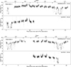 |
Fig. 1. XRISM Resolve and NuSTAR light curves in the 2−10 keV and 4−30 keV energy range, respectively, for observations 1 (top) and 2 (bottom) showing absorption dips at the start and end of the observations. The binning is 25 s in each panel. The thick tick marks at the top axis mark the start and end of phase-resolved intervals. |
The NuSTAR observations are simultaneous to the XRISM observations, but each observation covers only half the orbital period of the system. However, the availability of NuSTAR spectra for all orbital phases at least from one observation and the similarity of the two observations, as indicated by the XRISM light curves, made it possible to perform broadband spectral fits. In this work, we concentrated on analysing the persistent emission, and we refer the reader to Caruso et al. (in prep.) for a detailed analysis of the dips.
3.2. Spectral analysis
To inform our detailed analysis and determine the general properties of the plasma, we first extracted an aggregated spectrum for the persistent emission for each observation. We found that the continuum from the XRISM Resolve spectra could be satisfactorily fitted with a blackbody component (bb component in spex) modified by cold absorption from the interstellar medium (hot component in spex). However, the hard X-ray spectra available from the NuSTAR observations indicate that a second component is necessary to fit the hard X-rays. Therefore, we added a second component to the continuum consisting of Comptonisation of soft photons in a hot plasma using the blackbody as the source for the seed photons (comt component in spex). Thus, our Model 1 is hot*(bb+comt) in spex notation.
Similarly to previous observations from XMM-Newton and Chandra (Parmar et al. 2002; Xiang et al. 2009), the residuals show clear narrow and deep absorption features from highly ionised Fe (see Fig. 3). The unprecedented spectral resolution of XRISM Resolve reveals a clear blueshift in the Fe XXV and Fe XXVI lines with respect to their rest energy for the first time. In addition, the spin-orbit doublet of Fe XXVI is resolved into two distinct, narrow features. Given the excellent statistics of the spectra and the orbital modulation apparent in the light curves, we chose not to perform a detailed analysis of the aggregated spectra, and we continue instead with a discussion of our phase-resolved analysis in the remainder of this paper.
We note that previous spectral analyses of 4U 1624−49 with XMM-Newton and Chandra (Díaz Trigo et al. 2006; Xiang et al. 2007) included the contribution of a dust-scattering halo. This halo is produced by a dust cloud in the line of sight to the source, at a distance of approximately 15 kpc (Xiang et al. 2007), which scatters light from the source and delays the arrival of its emission by 1.6 ks seconds. Based on Fig. 7 from Xiang et al. (2007), the contribution of the scattering halo is significant up to ∼1′ in radius and decreases thereafter. Given that the PSF of XRISM, 1.3′, is significantly larger than that of Chandra, 0.5″, or XMM-Newton, 5″, we estimate that the inclusion of a dust-scattering-halo component is not needed for the analysis of the persistent phase spectra.
However, we note that this may not be the case when analysing the dipping spectra. In such a case, the time delay introduced by the scattering will result in emission from the persistent intervals scattered in during dipping intervals and such scattered emission from the persistent intervals may be significant compared to the low-flux characteristic of dipping intervals. The larger field of view of Xtend when compared with Resolve may also be helpful to fully characterise the halo contribution during that interval. We refer the reader to Caruso et al. (in prep.) for further discussion on this topic.
3.3. Phased-resolved spectral analysis
We next used the orbital period of the source of 20.87 h to slice the persistent emission into five intervals, each covering 0.15 in orbital phase (p0–p4, with p0 starting at phase 0 and p4 ending at phase 0.75), for a total of three quarters of the full orbit. We used the same ephemeris (2024-03-30 03:57:15 UT as the start time of p0 for Obs 1) for the two observations to make sure that the same orbital phases were covered. We define φ0 such that intervals p0–p4 do not include episodes of deep dipping in any of the observations (see Fig. 1). This is to avoid the low ionisation plasma present during dips and associated with the accretion stream or disc bulge (Boirin et al. 2005; Díaz Trigo et al. 2006) affecting our characterisation of the highly ionised plasma.
We also note that inspection of the continuum parameters and residuals for the phase-resolved intervals indicates that observations 1 and 2 have similar spectra within the uncertainties. Therefore, we merged the event files of the two observations to increase the statistics, and we re-extracted the phase-resolved spectra for the merged event file, to which we refer in the remainder of this paper.
3.3.1. Continuum fits
We first re-fitted the XRISM and NuSTAR spectra for each of the phase-resolved intervals (after merging the two observations) with the same continuum as that used for the phase-aggregated spectrum (Model 1). Despite having broadband spectra, we found that the opacity of the Comptonisation component is unconstrained in the fits. Therefore, we fixed the opacity to a value of ten, which resulted in values for the temperature of the seed photons and of the electrons similar to those recently obtained by Gnarini et al. (2024).
This model fits the spectra of the five intervals well. As an example, Fig. 2 shows the broadband fit for interval p2, with clear narrow residuals at the Fe K energy region. A more detailed look at the residuals in the Fe Kα region for all intervals (Fig. 3) shows additional important differences among intervals. First, blueshifts are apparent for all lines with respect to their rest energy, but the blueshifts differ among the intervals, with p0 and p4 showing the smallest blueshift and p2 the largest.
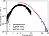 |
Fig. 2. XRISM Resolve and NuSTAR spectra for interval p2 fitted with Model 1 (hot*(bb+compt); see text). |
A prominent feature at ∼6.66 keV is present only in intervals p0 and p4, most likely due to the presence of the intercombination line of Fe XXV or Fe XXIV. In addition, the Lyα1 line shows an apparent blue wing in p0 and a double peak, reminiscent of two components with different velocities, in p4.
The larger column density of Fe XXVI in intervals p0 and p4 is confirmed by the presence of transitions up to Lyγ in those intervals. This larger column density could be caused by a plasma with lower ionisation for which ions that were fully stripped in intervals p1–p3 have now gained an electron and become visible.
Finally, the ratio of the lines in the Fe XXVI spin-orbit doublet shows some differences among intervals. This can point to different solid angles and fraction of scattered emission of the plasma. However, the fact that Lyα2 is deeper than Lyα1 for interval p2 (against the expected 1:2 ratio for Lyα2:Lyα1) may also point to saturation effects derived from large column densities.
3.3.2. Fits to individual species
To evaluate the effect of saturation on the lines in the fits with photoionised plasmas, we first performed fits to Fe XXV and Fe XXVI lines separately and for two different energy ranges: the 6.5−9 keV energy range, which includes all important transitions, and the 7.5−9 keV energy range, which does not include the Kα (Heα for Fe XXV or Lyα for Fe XXVI) components that we suspect are saturated. For this, we used the slab component in spex, in which the column density of each species can be fitted independently by taking the width and shift of lines into account. This component treats the absorption by a thin slab composed of different ions in a simplified manner and is a good approximation as long as the slab is not too large (Kaastra et al. 2002). To improve the measurement of the line shifts, we also used the Ni XXVII, and Ni XXVIII species that we do not expect to be saturated. Due to the very narrow energy range used for this test, we used a simplified continuum of a blackbody with temperature and normalisation as free parameters for each interval. Table 2 shows the results of the fits for all intervals for the 7.5−9 keV energy range.
Spectral fits of Fe XXV, Fe XXVI, Ni XXVII, and Ni XXVIII species for p0–p4 intervals with the slab component (see text).
When the Kα transitions are included in the fit, the fitted column densities are lower, and the Kβ transitions are not well fitted, indicating line saturation that is not being accounted for with this simple model; this is likely because the presence of scattered radiation does not allow the absorption lines to reach zero flux. Because of this saturation effect, we first focused on the values obtained from the fits to the 7.5−9 keV energy range, which allowed us to obtain a first estimate of the column densities and velocities with this simple model.
An increase of column density of both Fe XXV and Fe XXVI is observed in intervals p0 and p4, as expected from Fig. 3. In addition, a clear modulation is observed in the shift of the lines, with a maximum of ∼450 km s−1 observed during p2.
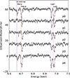 |
Fig. 3. Residuals in Fe Kα energy range for intervals p0–p4 after fitting the continuum. The y-scale has been shifted for p0–p3 for clarity. |
We note that we also attempted to fit each species separately. However, due to the larger uncertainties of the width and shift of the lines in the fits to the individual species, we cannot make any definite conclusion at this stage on whether the location of the individual species is different. Therefore, we only show the joint fit to the Fe Kβ, Ni XXVII, and Ni XXVIII lines, which allowed us to reduce the uncertainties in the velocity shift compared to those obtained when fitting each species individually.
3.3.3. Fits with photoionised models
To provide a more detailed characterisation of the ionised plasma, we next substituted the slab component by the pion component in spex (Mehdipour et al. 2016). This component uses the ionising radiation from the continuum component self-consistently, so the ionisation balance and the spectrum of the photoionised plasma always correspond to the fitted continuum; this is particularly adequate when broadband continua are available, as was the case in this work. We first allowed the column density, ionisation parameter, velocity width, and velocity shift of the pion component to vary (hot*pion1*(bb+comt) in spex, hereafter Model 2a). This model significantly improves the fit compared to Model 1 for all intervals (Δ C-stat. between 183 and 930 for 4 additional d.o.f.), with the largest improvement observed for intervals p0 and p4. However, as indicated before, the line ratio of the Fe XXVI spin-orbit doublet differs from the expected 2:1 ratio in all intervals and even inverts in p1, p2, and p4. Therefore, we also tried variations of Model 2a leaving the covering factor (Model 2b) or the solid angle (Model 2c) as free parameters in the pion component. A covering factor under one implies that the ‘uncovered’ continuum emission does not undergo absorption by the photoionised plasma and therefore mimics scattered continuum by the photoionised plasma. In contrast, a solid angle larger than zero includes emission from the absorbing plasma but does not include the scattered continuum. In particular, in Model 2c the emitting plasma is forced to have the same parameters (column density, ionisation parameter, velocity broadening, and velocity shift) as the absorbing plasma. This implies that we only include emission from the plasma that is also absorbing, and not from plasma that is, for example, in other orbital phases and impossible to see via absorption. We find that the two modified models improve the fits in general. For p4, the improvement is large, with Δ C-stat. of 138/108 for Models 2b and 2c for one additional d.o.f., respectively. For intervals p0–p3, the improvement is less prominent, with Δ C-stat. between ∼12 and 45 for one additional d.o.f. The results of the fit for Models 2b and 2c are shown in Tables 3 and 4, respectively. Fig. 4 shows the fit with the different models in the relevant Fe K region for all intervals.
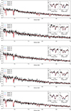 |
Fig. 4. Spectra for intervals p0 to p4 (top to bottom, respectively) with Models 2a, 2b and 2c overplotted in cyan, blue and red, respectively (see Tables 3 and 4 for fitted parameters). The insets show a detail of the Fe XXV and Fe XXVI Kα regions highlighting the different prediction of the three models for the Fe XXVI spin-orbit doublet ratio. |
Spectral fits of p0–p4 intervals with Model 2b (see text).
Spectral fits of p0–p4 intervals with Model 2c (see text).
Looking at interval p4, the improvement of Models 2b and 2c with respect to 2a is due to the former models being able to capture the high column density of the absorber. As indicated in previous section, the column density for Fe XXV and Fe XXVI is the highest for this interval based on fits to the Kβ transitions. The Kα lines are saturated, but Model 2a is not able to account for that because the lines do not reach zero intensity, likely due to scattered emission from the wind3 setting a ‘floor’ for the lines higher than zero. In contrast, both Models 2b and 2c ‘set such a floor’, with Model 2b doing it via the uncovered emission and Model 2c via plasma re-emission. Interestingly, these two models give similar improvements in C-stat. Model 2c is able to better account for the stronger Lyα2 line compared to Lyα1 in p2, but it also predicts a stronger Lyα2 line in p0 and p3, in which it is not observed. Model 2b provides a better overall fit to p4, although the structure (double-peak) of the Lyα1 transition is better accounted for in Model 2c.
Despite the described limitations, Models 2b and 2c generally provide a good description of the data. Allowing both the covering factor and the solid angle to vary at the same time only introduces improvements of the fit of Δ C-stat. = 2−3 for one additional d.o.f.. We also attempted to verify Model 2b by substituting the covering factor (i.e. leaving it at one) by an independently added diffuse scattered component (hot*pion*(bb+comt)+hot(bb+comt), Model 3). This model provides fits of similar quality to Model 2b (with Δ C-stat. = 0−9 for one additional d.o.f.). We also tried to add a plasma-re-emission component with parameters independent of the absorbing plasma to Model 3 to account for the averaging of plasma emission from other parts of the disc, but we only obtained a fit improvement for intervals p1 and p3, indicating that we may have reached some degeneracy in the fits. Overall, we observe scattering fractions of ∼20−30%, which match the amount of ‘uncovered’ emission in Model 2b of 17−35% and the solid angle of ∼10−20% in Model 2c well, thus indicating that with the current data we cannot distinguish further between alternative models. A potential exception is interval p0, for which a blue wing in the Lyα1 transition is not accounted for by Models 2b–2c (see below).
During p1–p3, the ionisation and column density of the absorber are consistent among the three intervals within the errors, and the velocity width is generally small (∼50−110 km s−1) and shows a trend of increasing width from p1 to p3. The most remarkable change among these intervals is the blueshift of the absorber, which changes as a function of phase, indicating orbital modulation and reproducing the behaviour already observed in the fits to the individual lines in the previous section.
For intervals p0 and p4, as we leave and approach the dipping phase, respectively, the ionisation of the observer significantly decreases compared to p1–p3. This decrease of ionisation may account for the increase of column density in Fe XXV and Fe XXVI observed in Table 2. For p0 the shift of the absorber is also remarkably larger (by ∼45 km s−1) for Models 2b–2c compared to that found with fits to the individual lines. This and the lower ionisation of the plasma for these intervals may be pointing out to the presence of additional absorbers.
Therefore, we next attempted to add a second absorber for p0 (for which the differences in log ξ and v are larger) to test the hypothesis that the lower ionisation of the plasma is actually caused by a mix of two plasmas, one highly ionised and similar to that found in p1–p3 and another one with lower ionisation resulting from, for example, some material from the dipping phase spreading outside of such a phase. To constrain the fit we fixed log ξ = 4 erg cm s−1 and σv = 50 km s−1 for the first absorber, under the assumption that such an ionised absorber does not significantly change among intervals. Adding a second absorber significantly improves the quality of the fit (ΔC-stat. = 38 and 68 for 3 d.o.f. with respect to Models 2b and 2c, respectively) by partially fitting the blue wing of the Lyα1 line (see Table 5 and Fig. 5). The two absorbers had velocities of ∼−310 and −140 km s−1 at this point; thus, the low-ionisation absorber adopts a velocity closer to that obtained with the fit to the Kβ lines, although we suspect that we have reached some degeneracy in the fits. We also attempted to add a second absorber for p4, but in this case the fit does not significantly improve with respect to that with one absorber.
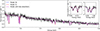 |
Fig. 5. Spectrum for interval p0 with the model with two absorbers displayed in Table 5 overplotted in magenta for comparison with Models 2b and 2c (which have only one absorber, overplotted in blue and in red), respectively (see Tables 3, 4 and 5 for fitted parameters). The insets show details of the Fe XXV and Fe XXVI Kα regions highlighting the different predictions of the three models for the Fe XXVI spin-orbit doublet ratio. |
4. Discussion
The unprecedented resolution of the microcalorimeter Resolve on board XRISM enabled us to determine for the first time a significant blueshift in the highly photoionised absorber previously seen in 4U 1624−49, indicating the presence of an outflow with a column density of ∼1−2 × 1023 cm−2. A phase-resolved analysis shows that the highly ionised plasma is present in all intervals of the persistent emission. The plasma consistently shows a blueshift in all intervals, and the value is modulated by the orbital phase. The velocity width is generally low, down to values of 50 km s−1 in p1, indicating minimal sheer and/or turbulence, although it increases up to ∼150 km s−1 in p4, perhaps due to to an increase of turbulence as we approach the dipping phase. Solid angles of 10−20% are found with Model 2c, which is consistent with an equatorial wind, and with estimates from the solid angle of the wind in the LMXB GX 13+1 (Xrism Collaboration 2025). With Model 2b, we find covering factors of ∼65−83%, which are smaller for p2 and p3 compared to p0 and p4; that is, the uncovered (or scattered) emission is larger for p2 and p3. If we only fit the XRISM Resolve data with an additional scattered component, we find scattering fractions of 20−30%, which are again larger for p2 and p3 compared to p0 and p4. We interpret this as p2 and p3 (at orbital phases 0.30−0.45 and 0.45−0.60, respectively) seeing more diffuse scattered emission from the opposite part of the disc (phases 0.80−0.95 and 0.95−1.10) due to the opacity of additional material present during the dipping phase, which especially affects p2. However, we emphasise that in reality we expect both scattered continuum and plasma re-emission (including that from plasma in other parts of the disc). Therefore, the overall scattering fraction is likely to be slightly less than that found when only one of the components (continuum scattering or plasma re-emission) is included. Interval p1 is an outlier with respect to such trends, but it also shows continuum parameters deviating from those seen during the other intervals. We attribute the outlier behaviour of p1 to the worse statistics of that interval because of observation 2 largely missing such a phase, or to a higher short-term flux during observation 1 (see Fig. 1). Moreover, fits with the continuum tied among intervals p1–p3 result in similar values for the absorbers to those observed in Models 2b–2c. Therefore, overall changes in the scattering and absorption in the line of sight, rather than source intrinsic variability, are likely to fully cause the variability across the orbital phase and naturally explain why the light curves remain stable over periods of days.
In interval p0, a second, lower ionisation plasma appears with a lower outflow velocity than the highly ionised plasma. Since in p0 we leave the dipping phase, such a plasma may be the less ionised component typically seen during dips (Díaz Trigo et al. 2006), which spreads over to p0 (see Caruso et al., in prep. for the detailed analysis of the dips). Introducing this second absorber allows the highly ionised plasma to better account for the blue wing of the Fe XXVI Lyα1 transition (although not completely). We note that blue wings associated with the Fe XXVI Lyα1 transition are apparent in other XRISM observations of LMXBs (see Fig. 6 of Tsujimoto et al. 2025). The phase-resolved analysis performed here indicates that despite blue wings being predicted by magnetic-wind models (e.g. Fukumura et al. 2017), such an association is unlikely in this case, since the wing should be seen across all phase-resolved spectra. Instead, since blue wings are more apparent in observations in which high plasma opacities are found (Xrism Collaboration 2025), we suggest that our relatively simple models assuming optically thin, slab-like plasmas are not able to fully account for the complexity of radiation transfer and scattering effects at high opacities. We emphasise that sources such as 4U 1624−49 are ideal for understanding these effects for the first time; this is due to their stable luminosity and accretion state allowing phase-resolved studies that isolate the phenomenology due to the orbital dependence of the photoionised plasmas.
4.1. Radial velocity
The radial-velocity (RV) dependence on the orbital phase shows a clear sinusoidal pattern (see Fig. 6). However, the values of the velocity for interval p0 significantly differ for the different models. We measure −150 ± 19 km s−1 when using the Fe XXV and Fe XXVI Kβ transitions (Table 2) and −194 ± 8 km s−1 when using Model 2c (Table 4). However, the largest difference is found for the fit with two pion components, in which the highly ionised component (with ionisation and velocity width similar to the p1–p3 intervals) results in an outflow velocity of −307 ± 44 km s−1 (Table 5). Fitting the data with a sine curve thus results in different values for the amplitude and the offset. We obtain RV amplitudes of 229 ± 14 km s−1, 200 ± 6 km s−1, and 177 ± 9 km s−1 and RV offsets of −245 ± 8 km s−1, −270 ± 4 km s−1, and −285 ± 7 km s−1 for the three outlined methods, respectively.
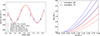 |
Fig. 6. Left: Best-fit values of velocity shift of the highly ionised absorber as a function of orbital phase as determined with three different methods (see text) and the best-fit model (red) using the values from Model 2c with two absorbers for p0 (dark blue). Right: Allowed masses for companion star for two different inclinations based on the best-fit model from the RV curve. |
Spectral fits of the p0 interval with the hot*pion2*pion1*(bb+comt) model.
The RV offset is large, regardless of the method, and even after considering the sum of the gain uncertainty and XRISM motion around the Earth (averaging to 0 km s−1), the Earth’s motion around the Sun (23.8 and 23.0 km s−1 during the first and second observations, respectively) and the Sun’s motion with respect to the Local Standard of Rest (2.8 km s−1). Since the companion of 4U 1624−49 is not well characterised due to the high extinction, we instead used that 4U 1624−49 follows the Galactic rotation except for the natal kick and that the Galactic rotation curve is flat at 220 km s−1 (e.g. Mróz et al. 2019) to determine the estimated velocity. At a distance of ∼15 kpc (Xiang et al. 2007), the relative velocity of 4U 1624−49 is then −3 km s−1. Assuming a natal kick of 54 km s−1 (Hobbs et al. 2005) and accounting for all motions, we obtain a velocity of the absorber of ∼200−320 km s−1, thus firmly establishing the presence of a highly ionised outflow in 4U 1624−49.
We next used the RV amplitude to set some constraints on the mass of the companion. We determine the mass function as f = K3 Porb/2πG, where K is the semi-amplitude of the RV curve and G is the gravitational constant. This results in values of f of 1.08, 0.71, and 0.50 M⊙ for the three methods. We assumed an inclination between 60° and 75° from the presence of absorption dips and the absence of eclipses (Frank et al. 1987). Using the relation  , we were then able to determine the mass of the companion as a function of the NS mass. For plausible values of the NS mass of 1.3−1.5 M⊙, we obtained a mass for the companion star near to 1 M⊙ only when two absorbers were considered for p0: namely, a mass of the companion of 1.3−1.4 M⊙ for an inclination of 75°. In contrast, for a mass function of 0.71 the corresponding companion star masses are > 1.8 M⊙. Therefore, the scenario in which a second intervening absorber with lower velocity appears in the line of sight between the wind and us is more supportive of 4U 1624−49 being a LMXB, although an intermediate X-ray binary could be a possibility for one absorber.
We note that the while K corresponds to the RV semi-amplitude of the NS, in reality we measured absorption in a wind launched far from the NS. However, we estimate that this does not introduce systematics in the measurement due to the fact that we used absorption lines and that the wind is most likely axisymmetric and centred around the NS. While a precessing disc could still introduce some asymmetry, such a disc has not been claimed so far.
Finally, we also note that the zero orbital phase is offset by ∼0.1 in the RV curve, indicating that with our definition of zero phase (see Sect. 3.3), p0 would be almost centred around the eclipse. Methods including Doppler tomography may help us clarify the emission zones further.
4.2. Origin of the wind
Based on the orbital modulation and the RV analysis performed in Sect. 4.1, we estimate the velocity of the outflow to be ∼200−320 km s−1. The cleanest characterisation of the outflow can be made at the orbital phase farthest from the dip, that is, during interval p2, due to the absence of other intervening absorbers. Therefore, we used the source luminosity, and column density and ionisation of the absorber obtained during that interval to estimate the launching radius of the outflow.
The luminosity of 4U 1624−49 reaches ∼6 × 1037 erg s−1 in these observations, corresponding to 0.32 LEdd for a typical NS mass of 1.4 M⊙. Using log ξ = Ln−1r−2, where n and r are the density and the launching radius of the wind, respectively, and considering Δr/r ≤ 1, we obtain that the wind is launched at a distance of ∼3.9 × 1010 cm. Considering a Compton radius of 1011 cm for a Compton temperature of ∼107 K (see Eq. 2.7 in Begelman et al. 1983), it follows that the wind is being launched at ∼0.39 of the Compton radius, in the region allowed for Compton heated winds. This is only slightly larger than the location estimated for the origin of the Fe XXVI absorption lines of 3 × 1010 cm based on previous phase-resolved analysis with Chandra/HETGS, for which no significant line shifts were observed (Xiang et al. 2009).
At such a large radius, the gravitational and transverse Doppler shift are expected to be negligible. Thus, the observed velocity is expected to correspond to the escape velocity of the wind. However, at a radius of 3.9 × 1010 cm, the escape velocity, estimated as  , where G is the gravitational constant, M is the mass of the NS, and r is the estimated wind-launching radius, is ∼980 km s−1; this is more than three times the outflow estimated velocity. This could indicate projection effects, albeit implying seeing the wind at a large offset angle, or some deceleration of the wind after launch. A third possibility is that the bulk of the ion column densities for the relevant ions is at a radius larger than the launching radius. In that case, the blueshift of the lines would be dominated by those at the radius where the column density peaks (see Tomaru et al. 2020, Fig. 6).
Remarkably, the width of the lines is only ∼50−70 km s−1 during p0–p2. This indicates that no stratification is present, thus supporting the origin of the wind as thermal pressure with the bulk of the wind located over a small range of radii. Moreover, the lines are also narrow when compared to other X-ray binaries already observed with XRISM (Tsujimoto et al. 2025). However, the changes observed throughout the orbit emphasise the need for phase-resolved spectroscopy to precisely determine the line widths. Not only do spectra aggregated throughout the orbit artificially broaden the lines due to the sum of different line shifts, we also demonstrate that at phases close to the dipping events additional absorbers and/or turbulence increase the line widths, which could be misinterpreted if their origin is uniquely attributed to the outflow. In addition, a larger width could arise due to saturation of the lines derived from large column densities if not properly accounted for.
We note that additional absorbers may not uniquely be related to dipping events locked in phase. For example, the light curve during intervals p0 and p4 does not show any strong absorption events reminiscent of dips. However, the spectroscopic analysis already reveals an increase in the column density of the absorber derived from a decrease of its ionisation probably due to mixing with material from the accretion stream or the bulge. If additional absorbers are behind the increase of the line width in p4, this could also explain the larger widths observed for the black hole 4U 1630−47 (Miller et al. 2025), for which an additional absorber was also seen in part of the orbit.
We finally estimated the mass outflow rate by making use of the precise knowledge of the luminosity (made possible by the accurate distance and the broadband spectral energy distribution measurements), and the measured ionisation parameter and solid angle. Again, we used the interval p2 with the most reliable parameters and obtain a mass-outflow rate of Ṁ ∼ nmpr2vout = 5−10 × 1016 g s−1 (with the higher estimate taking into account the outflow from both sides of the disc). This mass outflow rate is comparable to that estimated for GX 13+1 at a similar Eddington luminosity (Ueda et al. 2004).
4.3. Comparison to other systems
The XRISM PV phase included observations of two other high-inclination LMXBs for which winds had been already reported, GX 13+1 (e.g. Ueda et al. 2004) and Cir X-1 (e.g. Brandt & Schulz 2000).
For GX 13+1, previous observations at 0.3−0.4 LEdd had repeatedly shown a wind (Ueda et al. 2004; Allen et al. 2018) with a relatively high and changing column density (Díaz Trigo et al. 2012). The XRISM observation, during which the source had a luminosity near Eddington, revealed an unprecedented increase in the column density, making the wind optically thick and creating significant obscuration (Xrism Collaboration 2025). Interestingly, the wind observed in 4U 1624−49 is similar to that from previous observations of GX 13+1, indicating that at similar luminosities, winds are alike in terms of opacity, ionisation, and outflow velocity. Cir X-1 also showed a luminosity of ∼0.4 LEdd during the XRISM PV phase observation, and again the outflow velocity was ∼300 km s−1, although higher velocities had been observed in previous Chandra observations at higher luminosities (Brandt & Schulz 2000; Schulz & Brandt 2002).
Thus, remarkably, the outflow velocities observed for GX 13+1, Cir X-1, and 4U 1624−49 are very similar for luminosities of 0.3−0.4 LEdd, despite the large differences in the orbital period of these systems, ranging from 24 days to less than one day. Small differences could arise due to velocity projections for slightly different inclinations or different systemic velocities. However, the general trend points to these winds being launched via the same thermal-radiative pressure mechanism, for which the launching radius only depends on the spectral hardness and the source luminosity.
Similarly to what was observed by Chandra for Cir X-1, higher luminosities would result in higher outflow velocities (Brandt & Schulz 2000; Schulz et al. 2008), and therefore the higher luminosity of GX 13+1 in the XRISM observation would result in the appearance of a faster, broader outflow component (Xrism Collaboration 2025). However, we emphasise that blue wings are not necessarily associated with fast components, since for 4U 1624−49 a blue wing for the Fe XXVI Lyα1 component of the spin-orbit doublet is phase-dependent. If such a wing were due to the structure of the wind, and assuming that the wind would be axisymmetric, we would also expect to see it at other phases. An alternative origin for the blue wing could be the superposition of lower ionization, high column density, material from the accretion disc rim, and the accretion disc wind. In intervals approaching the absorption dip, the mixing of such components can result in different profiles depending on the line saturation and the velocity superposition of the two components. An increase of turbulence as we approach the dip could also explain the increase of line widths.
A strong scattering component is common to all the observed systems. This results in absorption lines not reaching zero intensity despite the large column densities. Including a scattered component in broadband spectra is, however, difficult due to the energy dependence of Compton scattering not being taken into account in a model that simply adds a fraction of the initial continuum. For 4U 1624−49, we find that allowing for a covering factor of the wind less than one improves significantly the fits, and we attribute it to the uncovered emission mimicking the scattered component. Overall, scattering fractions between 5 and 30% are reported and are consistent with the opacity expected from the wind and additional material at the disc rim.
Besides the scattered continuum, we expect that re-emission from the plasma reaches us from the entire disc, and therefore the re-emission should in principle correspond to relatively broad emission lines with lower velocity than the absorption lines. This seems to be the case for GX 13+1 (Xrism Collaboration 2025), which is consistent with interpretations based on previous low-resolution observations (Díaz Trigo et al. 2012). In contrast, for 4U 1624−49, we find that the changes in the ratio of the Fe XXVI spin-orbit doublet require a narrow-line re-emission to take place.
4.4. Limitations
The overall spectral analysis results in a relatively simple physical picture according to which a highly ionised thermal-radiative outflow is modulated by orbital motions and mixes with lower ionisation plasmas near the dipping phase, as shown for the particular case of p0. However, some additional plasma structure has likely not been captured with this simple model. Despite the excellent statistics of the observations presented here, the need to perform phase-resolved spectroscopy naturally reduces the overall statistics of each spectrum. The remaining small residuals indicate that we may be reaching the limit of these data when it comes to disentangling the highly ionised wind from the lower ionisation plasma expected from the accretion stream or material spreading from the bulge that causes the absorption during dips.
Acknowledgments
MDT thanks A. Gnarini and S. Bianchi for providing an accurate ephemeris for the dips of the IXPE observation and R. Tomaru for discussions on thermal winds. TY acknowledges support by NASA under award number 80GSFC24M0006. We thank the referee for a constructive and insightful report. MS acknowledges support by Grants-in-Aid for Scientific Research 23K03459 from the Ministry of Education, Culture, Sports, Science and Technology (MEXT) of Japan, and by Ehime University Grant-in-Aid Research Empowerment Program.
References
- Allen, J. L., Schulz, N. S., Homan, J., et al. 2018, ApJ, 861, 26 [Google Scholar]
- Begelman, M. C., McKee, C. F., & Shields, G. A. 1983, ApJ, 271, 70 [CrossRef] [Google Scholar]
- Boirin, L., Méndez, M., Díaz Trigo, M., Parmar, A. N., & Kaastra, J. 2005, A&A, 436, 195 [NASA ADS] [CrossRef] [EDP Sciences] [Google Scholar]
- Brandt, W. N., & Schulz, N. S. 2000, ApJ, 544, L123 [Google Scholar]
- Díaz Trigo, M., & Boirin, L. 2016, Astron. Nachr., 337, 368 [Google Scholar]
- Díaz Trigo, M., Parmar, A. N., Boirin, L., Méndez, M., & Kaastra, J. 2006, A&A, 445, 179 [NASA ADS] [CrossRef] [EDP Sciences] [Google Scholar]
- Díaz Trigo, M., Sidoli, L., Boirin, L., & Parmar, A. N. 2012, A&A, 543, A50 [NASA ADS] [CrossRef] [EDP Sciences] [Google Scholar]
- Fender, R., & Muñoz-Darias, T. 2016, Lect. Notes Phys., 905, 65 [NASA ADS] [CrossRef] [Google Scholar]
- Frank, J., King, A. R., & Lasota, J. P. 1987, A&A, 178, 137 [NASA ADS] [Google Scholar]
- Fukumura, K., Kazanas, D., Shrader, C., et al. 2017, Nat. Astron., 1, 0062 [NASA ADS] [CrossRef] [Google Scholar]
- Gnarini, A., Lynne Saade, M., Ursini, F., et al. 2024, A&A, 690, A230 [NASA ADS] [CrossRef] [EDP Sciences] [Google Scholar]
- Hobbs, G., Lorimer, D. R., Lyne, A. G., & Kramer, M. 2005, MNRAS, 360, 974 [Google Scholar]
- Kaastra, J. S., & Bleeker, J. A. M. 2016, A&A, 587, A151 [NASA ADS] [CrossRef] [EDP Sciences] [Google Scholar]
- Kaastra, J. S., Steenbrugge, K. C., Raassen, A. J. J., et al. 2002, A&A, 386, 427 [NASA ADS] [CrossRef] [EDP Sciences] [Google Scholar]
- Kilbourne, C. A., Sawada, M., Tsujimoto, M., et al. 2018, PASJ, 70, 18 [Google Scholar]
- Mehdipour, M., Kaastra, J. S., & Kallman, T. 2016, A&A, 596, A65 [NASA ADS] [CrossRef] [EDP Sciences] [Google Scholar]
- Miller, J. M., Raymond, J., Fabian, A., et al. 2006, Nature, 441, 953 [NASA ADS] [CrossRef] [Google Scholar]
- Miller, J. M., Mizumoto, M., Shidatsu, M., et al. 2025, ApJ, 988, L28 [Google Scholar]
- Mróz, P., Udalski, A., Skowron, D. M., et al. 2019, ApJ, 870, L10 [Google Scholar]
- Muñoz-Darias, T., Díaz Trigo, M., Done, C., Ponti, G., & Tomaru, R. 2026, Space Sci. Rev., submitted [arXiv:2601.05319] [Google Scholar]
- Neilsen, J., & Homan, J. 2012, ApJ, 750, 27 [NASA ADS] [CrossRef] [Google Scholar]
- Parmar, A. N., Oosterbroek, T., Boirin, L., & Lumb, D. 2002, A&A, 386, 910 [NASA ADS] [CrossRef] [EDP Sciences] [Google Scholar]
- Ponti, G., Fender, R. P., Begelman, M. C., et al. 2012, MNRAS, 422, L11 [NASA ADS] [CrossRef] [Google Scholar]
- Porter, F. S., Kilbourne, C. A., Chiao, M. P., et al. 2025, J. Astron. Telesc. Instrum. Syst., 11, 042016 [Google Scholar]
- Schulz, N. S., & Brandt, W. N. 2002, ApJ, 572, 971 [Google Scholar]
- Schulz, N. S., Kallman, T. E., Galloway, D. K., & Brandt, W. N. 2008, ApJ, 672, 1091 [Google Scholar]
- Smale, A. P., Church, M. J., & Bałucińska-Church, M. 2001, ApJ, 550, 962 [NASA ADS] [CrossRef] [Google Scholar]
- Tashiro, M., Kelley, R., Watanabe, S., et al. 2025, PASJ, 77, S1 [Google Scholar]
- Tomaru, R., Done, C., Ohsuga, K., Odaka, H., & Takahashi, T. 2020, MNRAS, 497, 4970 [NASA ADS] [CrossRef] [Google Scholar]
- Trueba, N., Miller, J. M., Fabian, A. C., et al. 2020, ApJ, 899, L16 [Google Scholar]
- Tsujimoto, M., Enoto, T., Díaz Trigo, M., et al. 2025, PASJ, accepted [arXiv:2503.08254] [Google Scholar]
- Ueda, Y., Murakami, H., Yamaoka, K., Dotani, T., & Ebisawa, K. 2004, ApJ, 609, 325 [Google Scholar]
- Wachter, S., Wellhouse, J. W., Patel, S. K., et al. 2005, ApJ, 621, 393 [NASA ADS] [CrossRef] [Google Scholar]
- Woods, D. T., Klein, R. I., Castor, J. I., McKee, C. F., & Bell, J. B. 1996, ApJ, 461, 767 [NASA ADS] [CrossRef] [Google Scholar]
- Xiang, J., Lee, J. C., & Nowak, M. A. 2007, ApJ, 660, 1309 [Google Scholar]
- Xiang, J., Lee, J. C., Nowak, M. A., Wilms, J., & Schulz, N. S. 2009, ApJ, 701, 984 [NASA ADS] [CrossRef] [Google Scholar]
- Xrism Collaboration (Audard, M., et al.) 2025, Nature, 646, 57 [Google Scholar]
We remark that emission from scattering in the wind is local to the source. This component is different to the previously observed dust scattered emission (see Sects. 1 and 3.2), which arises through scattering of the overall source emission in dust clouds in the interstellar medium along the line of sight.
All Tables
Spectral fits of Fe XXV, Fe XXVI, Ni XXVII, and Ni XXVIII species for p0–p4 intervals with the slab component (see text).
All Figures
|
Fig. 1. XRISM Resolve and NuSTAR light curves in the 2−10 keV and 4−30 keV energy range, respectively, for observations 1 (top) and 2 (bottom) showing absorption dips at the start and end of the observations. The binning is 25 s in each panel. The thick tick marks at the top axis mark the start and end of phase-resolved intervals. |
| In the text | |
|
Fig. 2. XRISM Resolve and NuSTAR spectra for interval p2 fitted with Model 1 (hot*(bb+compt); see text). |
| In the text | |
|
Fig. 3. Residuals in Fe Kα energy range for intervals p0–p4 after fitting the continuum. The y-scale has been shifted for p0–p3 for clarity. |
| In the text | |
|
Fig. 4. Spectra for intervals p0 to p4 (top to bottom, respectively) with Models 2a, 2b and 2c overplotted in cyan, blue and red, respectively (see Tables 3 and 4 for fitted parameters). The insets show a detail of the Fe XXV and Fe XXVI Kα regions highlighting the different prediction of the three models for the Fe XXVI spin-orbit doublet ratio. |
| In the text | |
|
Fig. 5. Spectrum for interval p0 with the model with two absorbers displayed in Table 5 overplotted in magenta for comparison with Models 2b and 2c (which have only one absorber, overplotted in blue and in red), respectively (see Tables 3, 4 and 5 for fitted parameters). The insets show details of the Fe XXV and Fe XXVI Kα regions highlighting the different predictions of the three models for the Fe XXVI spin-orbit doublet ratio. |
| In the text | |
|
Fig. 6. Left: Best-fit values of velocity shift of the highly ionised absorber as a function of orbital phase as determined with three different methods (see text) and the best-fit model (red) using the values from Model 2c with two absorbers for p0 (dark blue). Right: Allowed masses for companion star for two different inclinations based on the best-fit model from the RV curve. |
| In the text | |
Current usage metrics show cumulative count of Article Views (full-text article views including HTML views, PDF and ePub downloads, according to the available data) and Abstracts Views on Vision4Press platform.
Data correspond to usage on the plateform after 2015. The current usage metrics is available 48-96 hours after online publication and is updated daily on week days.
Initial download of the metrics may take a while.