© The Authors 2026

1. Introduction

Satellite measurements near 1 au from the Sun and beyond have revealed that solar wind (SW) turbulence is weakly compressible, with density fluctuations that are typically less than 10% of the background density, and subsonic velocity fluctuations δu, with turbulent sonic Mach numbers M_S = δu/c_S ≲ 0.1, where c_S is the sound speed (Roberts et al. 1987; Montgomery et al. 1987; Matthaeus et al. 1990, 1991). These observations stimulated the development of nearly incompressible (NI) models of SW turbulence, based on the M_S ≪ 1 assumption. In the M_S ≪ 1 regime, compressible magnetohydrodynamic (MHD) equations can be expanded about a low-frequency incompressible state, with small amplitude high-frequency compressible corrections quasi-linearly coupled to the dominant incompressible flow (Matthaeus & Brown 1988; Matthaeus et al. 1991).

The SW dynamics is also affected by the strong interplanetary magnetic field, making turbulence anisotropic (Shebalin et al. 1983; Horbury et al. 2008; Wicks et al. 2010; Adhikari et al. 2024), and sub-Alfvénic, with turbulent Alfvén Mach numbers M_A = δu/c_A ≪ 1, where c_A is the Alfvén speed. Early NI models assumed M_A ∼ 𝒪(1), but extensions were developed that incorporate the M_A ≪ 1 condition, together with M_S ≪ 1 and varying plasma beta β = 2 c_S²/c_A² (Zank & Matthaeus 1992b, 1993; Bhattacharjee et al. 1998; Hunana & Zank 2010; Zank et al. 2017). The main conclusion drawn from these NI models is that subsonic sub-Alfvénic turbulence exhibits a 2D + slab structure, meaning that turbulent fluctuations consist of a majority of low-frequency 2D incompressible component, plus a minority of high-frequency 3D waves. Alongside NI models, purely incompressible theories of MHD turbulence have also been developed, including critically balanced turbulence (Goldreich & Sridhar 1995; TenBarge & Howes 2012) and reflection-driven turbulence (Verdini et al. 2009; Chandran & Perez 2019), successfully describing some of the main features of the weakly compressible SW turbulence.

The NI turbulent regime described so far potentially breaks down near the Sun, where turbulent velocity fluctuations are expected to increase in amplitude (Cranmer et al. 2017; Adhikari et al. 2020, 2022), and β is small (Kasper et al. 2021), implying c_S ≪ c_A. This results in a larger M_S, suggesting that turbulence might become more compressible near the Sun. Parker Solar Probe (PSP) measurements have recently shown that SW turbulence becomes transonic at about 11 R_⊙ (solar radii) from the Sun, where M_S ∼ 1 and M_A ≪ 1 (Zhao et al. 2025). This transition from a subsonic to a transonic turbulent regime is accompanied by a significant increase in density fluctuations, up to more than 20% of the background density.

Recent MHD simulations of subsonic turbulence have revealed that turbulent fluctuations mainly consist of low-frequency quasi-2D modes, rather than waves (Gan et al. 2022; Arrò et al. 2025). Low-frequency fluctuations are typically interpreted as coherent structures (Karimabadi et al. 2013; Pezzi et al. 2017; Papini et al. 2021; Arrò et al. 2023, 2024; Espinoza-Troni et al. 2025) produced by an inverse energy cascade (Arrò et al. 2025). The prevalence of low-frequency quasi-2D fluctuations over Alfvén waves (AWs), slow modes (SMs), and fast modes (FMs) is consistent with NI models of turbulence (Zank & Matthaeus 1992b, 1993; Zank et al. 2017), and with SW observations (Perrone et al. 2016; Roberts et al. 2017; Zhao et al. 2023; Zank et al. 2024). However, it is unclear whether this picture of turbulence continues to hold also in the newly observed M_S ∼ 𝒪(1) near-Sun regime, and to our knowledge, no model of transonic SW turbulence has ever been developed.

In this work, we studied transonic sub-Alfvénic turbulence using a 3D MHD simulation initialized with typical near-Sun SW parameters. We find that even in the transonic regime, turbulence is dominated by low-frequency quasi-2D incompressible structures, while compressible fluctuations are a minor component in the form of low-frequency SMs and high-frequency FMs. These results are consistent with a new MHD model of transonic sub-Alfvénic turbulence (TsAT) that we derived, showing that turbulence in the M_S ∼ 𝒪(1), M_A ≪ 1 regime is effectively NI, with a 2D + slab structure, similarly to subsonic turbulence.

2. Simulation setup

We performed our simulation using the MHD code Athena++ (Stone et al. 2020). We considered a domain of size L_z = 3L_y = 3L_x = 6 π (in arbitrary units L₀), sampled by a uniform periodic mesh with 256 × 512² points. The plasma is initially at rest, with uniform density ρ₀ and guide field ${\mathbf{B}}_0=B_0\widehat{\mathbf{z}}$. Pressure P is isothermal, with β = 2 c_S²/c_A² = 0.045. Turbulence is driven using the Langevin antenna method (TenBarge et al. 2014), with driving frequency ω₀ = 0.8 τ_A⁻¹ and decorrelation rate γ₀ = −0.7 τ_A⁻¹ (where τ_A = L₀/c_A). Injected velocity and magnetic field fluctuations are incompressible¹ and polarized in the plane perpendicular to B₀, with 1 ≤ k_∥L_z/2π ≤ 3 and 1 ≤ k_⊥L_x/2π ≤ 4, where k_∥ and k_⊥ are wavenumbers parallel and perpendicular to B₀. Viscous and resistive dissipation are included, with kinetic and magnetic Reynolds numbers R_e = R_m = 4000. The continuous driving produces a quasi-stationary turbulent state after about 20 τ_A, characterized by density, velocity, and magnetic field fluctuations with rms amplitudes δρ_rms/ρ₀ ≃ 0.22, δu_rms/c_A = M_A ≃ 0.155, and δB_rms/B₀ ≃ 0.153. The turbulent regime we considered is that of strong turbulence, as magnetic and velocity fluctuations are large enough to make nonlinear effects dominant. Velocity fluctuations are transonic, with M_S = δu_rms/c_S ≃ 1.03. We drive turbulence to be imbalanced, with cross-helicity ${\sigma }_C=⟨2\mathbf{u}·\delta \mathbf{B}/\sqrt{\rho }⟩/⟨u^2+\delta B^2/\rho ⟩\simeq 0.64$, where δB = B − B₀, and ⟨ ⋅ ⟩ is the box average. Imbalanced turbulence with σ_C > 0 is obtained by injecting more energy in the form of fluctuations with k_∥ > 0, and less energy into modes with k_∥ < 0 (TenBarge et al. 2014). These parameters are consistent with observations of near-Sun transonic sub-Alfvénic turbulence (Zhao et al. 2025).

3. Results

In this section we analyze the spectral properties of our turbulence simulation in wavenumber-frequency space, investigating the presence of waves and structures. Then we derive a new MHD model of transonic sub-Alfvénic turbulence to interpret our numerical results.

Figure 1 shows the temporal evolution of magnetic and kinetic energy variations ΔE_mag = E_mag(t)−E_mag(0) and ΔE_kin = E_kin(t)−E_kin(0) (in ρ₀ c_A² L₀³ units). We see that both energies grow and saturate after about 20 τ_A, indicating that turbulence has reached a quasi-stationary state (green shaded area). Figures 2a and b show (k_∥,  ω) and (k_⊥,  ω) projections of the magnetic field wavenumber-frequency spectrum P_B (where ω is the frequency), calculated over time interval [20 τ_A,  120 τ_A], with data sampled every Δt = 0.1 τ_A. The two projections correspond to P_B(k_∥,  ω) = ∫P_B(k_⊥,  k_∥,  ω) dk_⊥ and P_B(k_⊥,  ω) = ∫P_B(k_⊥,  k_∥,  ω) dk_∥. Similarly to subsonic turbulence, we find that in the transonic regime most magnetic field fluctuations correspond to low ω modes, while AWs, SMs, and FMs (dashed lines) are a minor component. Low ω fluctuations are highly anisotropic, with a much wider distribution in k_⊥ than in k_∥, implying a quasi-2D geometry. Since low ω fluctuations do not follow the dispersion relations of waves, we call them non-wave modes (NWMs). The spectrum P_B(k_∥,  ω) is skewed toward positive ω because of the high σ_C, making turbulence imbalanced (Lugones et al. 2019; Arrò et al. 2025). The observed energy distribution is consistent with critically balanced turbulence, as discussed in more detail in Appendix A. Figures 2c–d show (k_∥,  ω) and (k_⊥,  ω) projections of the density wavenumber-frequency spectrum P_ρ. We see that even density fluctuations mainly consist of low ω quasi-2D NWMs, dominating over SMs and FMs. To understand whether NWMs are incompressible or compressible, we analyzed the velocity wavenumber-frequency spectrum, separating the velocity field u into its incompressible and compressible components, u_i and u_c, with ∇ ⋅ u_i = 0 and ∇ × u_c = 0 (Bhatia et al. 2012). The ratio of the rms amplitudes of u_c to u_i is δu_c, rms/δu_i, rms ≃ 0.15, meaning that incompressible fluctuations are globally stronger than compressible ones. Figures 2e and f show (k_∥,  ω) and (k_⊥,  ω) projections of the incompressible velocity spectrum P_ui, while panels (g) and (h) show the corresponding projections of the compressible velocity spectrum P_uc. We find that u_i is almost entirely made up of NWMs, with a small contribution from AWs, and little to no energy associated with SMs and FMs. On the other hand, u_c essentially consists of SMs and FMs. The (k_∥,  ω) projection of P_uc, panel (g), reveals the presence of SMs at low ω, and a regular wavy pattern extending toward higher ω, corresponding to the projection of FMs in the (k_∥,  ω) plane. The (k_⊥,  ω) projection of P_uc, panel (h), shows the presence of high-frequency FMs, and some energy distributed around low ω, corresponding to the projection of SMs in the (k_⊥,  ω) plane. Low-frequency SMs extend over a much narrower k_⊥ range and are much weaker in amplitude than incompressible NWMs observed over the same frequency range in P_ui. Therefore, we find that NWMs are incompressible and account for the majority of magnetic and density fluctuations.

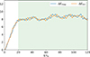Fig. 1. Temporal evolution of magnetic and kinetic energy variations ΔEmag and ΔEkin. The green shaded area represents the time interval used to calculate wavenumber-frequency spectra.

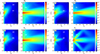Fig. 2. (k∥,  ω) and (k⊥,  ω) projections of PB (a)–(b), Pρ (c)–(d), Pui (e)–(f), and Puc (g)–(h). The dashed lines indicate dispersion relations of Alfvén waves (AW) and slow modes (SM) for k⊥ = 0, and fast modes (FM) for k∥ = 0.

A more quantitative estimate of the relative energy content of NWMs with respect to MHD waves can be obtained using the method described in Gan et al. (2022). This method consists in using wavenumber-frequency spectra, identifying as waves all those modes whose frequencies lie within 10% above and below the theoretical frequencies calculated from MHD dispersion relations of AWs, SMs, and FMs. The remaining energy is considered to be associated with NWMs. For this analysis, we excluded fluctuations lying in the injection range 1 ≤ k_∥L_z/2π ≤ 3, 1 ≤ k_⊥L_x/2π ≤ 4, as they are produced by the driver and do not develop as a consequence of the turbulent cascade. Using this approach, we find that AWs contain 36.79% of the total energy, SMs and FMs represent 1.02% and 0.53% of fluctuations, while the remaining 61.66% is made up of NWMs. This analysis shows the dominance of NWMs with respect to MHD waves, but we point out that the method we employed overestimates the energy content of AWs and SMs. The reason for this is that the dispersion relations of AWs and SMs at low k_∥ correspond to modes with very small ω that overlap with NWMs, lying in the same frequency range. Hence, part of the energy that this method considers to be associated with AWs and SMs in reality comes from NWMs.

To further assess the relative importance of waves with respect to NWMs, we compared the frequency spectra of u, u_i, and u_c at different propagation directions. Figure 3a shows the total velocity spectrum P_u, together with P_ui and P_uc, as functions of ω, for quasi-parallel modes with (k_⊥ = 1,  k_∥ = 10). We see that P_u has four peaks, two of which correspond to forward and backward propagating low-frequency SMs (black vertical dashed lines), with P_u ≃ P_uc, while the other two smaller peaks correspond to a superposition of high-frequency FMs and AWs (red and blue vertical dashed lines), with P_u ≃ P_ui. Thus, parallel propagating fluctuations are dominated by low ω compressible SMs, with a smaller high ω incompressible contribution from FMs and AWs. In Figure 3b we compare P_u, P_ui, and P_uc for quasi-perpendicular modes with (k_⊥ = 25,  k_∥ = 5). In this case, P_u ≃ P_ui, with a low ω peak that does not match the frequency of waves, and with negligible high ω compressible contributions from FMs. The largest peak corresponds to incompressible NWMs, representing the majority of perpendicular fluctuations. Finally, Figure 3c shows P_u, P_ui, and P_uc for oblique modes with (k_⊥ = 8,  k_∥ = 8). At this propagation direction, low frequencies are dominated by SMs, with P_ui ≃ P_uc, while higher frequencies show a significant contribution from AWs, with P_u ≃ P_ui, and from FMs, with P_ui ≃ P_uc. Hence, modes with k_⊥ ≫ k_∥ mainly consist of incompressible NWMs, while parallel and oblique fluctuations are essentially low-frequency SMs and high-frequency AWs and FMs.

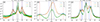Fig. 3. Frequency spectra of u, ui, and uc at (k⊥ = 1,  k∥ = 10) (a), (k⊥ = 25,  k∥ = 5) (b), and (k⊥ = 8,  k∥ = 8) (c). The vertical dashed lines indicate the corresponding frequencies of Alfvén waves (blue), slow modes (black), and fast modes (red).

Overall, we find that transonic sub-Alfvénic turbulence is mostly incompressible, with low-frequency quasi-2D NWMs dominating over waves. This seemingly counterintuitive behavior can be understood by taking the M_S ∼ 𝒪(1), M_A ≪ 1 limit of compressible MHD equations. Following the method outlined in Zank & Matthaeus (1993), we consider the normalized MHD equations

$$\begin{array}{cc}\hfill [{\partial }_t+(\mathbf{u}·\mathrm{\nabla })]\rho & =-\rho (\mathrm{\nabla }·\mathbf{u}),\hfill \end{array}$$(1)

$$\begin{array}{cc}\hfill \rho [{\partial }_t+(\mathbf{u}·\mathrm{\nabla })]\mathbf{u}& =-\frac{\mathrm{\nabla }P}{M_S^2}+\frac{1}{M_A^2}(\mathrm{\nabla }\times \mathbf{B})\times \mathbf{B},\hfill \end{array}$$(2)

$$\begin{array}{cc}\hfill [{\partial }_t+(\mathbf{u}·\mathrm{\nabla })]P& =-\gamma P(\mathrm{\nabla }·\mathbf{u}),\hfill \end{array}$$(3)

$$\begin{array}{cc}\hfill [{\partial }_t+(\mathbf{u}·\mathrm{\nabla })]\mathbf{B}& =(\mathbf{B}·\mathrm{\nabla })\mathbf{u}-\mathbf{B}(\mathrm{\nabla }·\mathbf{u}),\hfill \end{array}$$(4)

with γ being the polytropic index. In looking for turbulent solutions to these equations, three timescales are identified, namely T_T = λ/U₀, associated with the convective turbulent dynamics (where λ is a characteristic length scale of turbulence), the acoustic timescale T_S = λ/c_S, and the Alfvénic timescale T_A = λ/c_A. In the M_S ∼ 𝒪(1), M_A = ϵ ≪ 1 regime, Equation (2) becomes

$$\begin{array}{c}\hfill \rho [{\partial }_t+(\mathbf{u}·\mathrm{\nabla })]\mathbf{u}=-\mathrm{\nabla }P+\frac{1}{{ϵ}^2}(\mathrm{\nabla }\times \mathbf{B})\times \mathbf{B},\end{array}$$(5)

with T_T/T_S ∼ 1/M_S ∼ 𝒪(1) and T_T/T_A ∼ 1/M_A ≫ 1, implying that turbulence and SMs evolve on similar slow timescales, while AWs and FMs are much faster. With such timescale separation, we can assume that turbulent solutions consist of two components, a majority low-frequency turbulent state, and a minority component containing high-frequency fluctuations. Following this ansatz, the strategy is to find a low-frequency solution to MHD equations in the ϵ → 0 limit, and then to introduce small amplitude corrections, thus building an approximated solution valid for small but finite ϵ. The majority low-frequency component, labeled ∞, can be obtained using Kreiss’s theorem (Kreiss 1980), stating that time derivatives of low-frequency solutions must be independent of ϵ. We thus consider a low-frequency solution of the form

$$\begin{array}{c}\hfill \rho ={\rho }_0+ϵ{\rho }^{\infty },\mathbf{u}={\mathbf{u}}^{\infty },P=P_0+ϵP^{\infty },\mathbf{B}={\mathbf{B}}_0+ϵ{\mathbf{B}}^{\infty },\end{array}$$(6)

where ρ₀, P₀, and ${\mathbf{B}}_0=B_0\widehat{\mathbf{z}}$ are constants. Starting from ρ, its time derivative gives

$$\begin{array}{c}\hfill {\partial }_t{\rho }^{\infty }=-\mathrm{\nabla }·({\rho }^{\infty }{\mathbf{u}}^{\infty })-\frac{{\rho }_0}{ϵ}(\mathrm{\nabla }·{\mathbf{u}}^{\infty }).\end{array}$$(7)

In order for ∂_tρ^∞ to be independent of ϵ, u^∞ must be incompressible, i.e., ∇ ⋅ u^∞ = 0. Incompressibility results in the sourceless advection equation

$$\begin{array}{c}\hfill {\partial }_t{\rho }^{\infty }+({\mathbf{u}}^{\infty }·\mathrm{\nabla }){\rho }^{\infty }=0,\end{array}$$(8)

implying that if density fluctuations ρ^∞ are present in initial conditions, they are advected as a passive scalar, but no dynamical generation of ρ^∞ is possible. This allows us to set ρ^∞ = 0. Analogously, ∂_tP corresponds to a sourceless advection equation for P^∞, and we set P^∞ = 0. As we show later, density and pressure fluctuations are determined by the small amplitude compressible corrections to the ∞ component. The time derivative of u gives

$$\begin{array}{cc}\hfill {\partial }_t{\mathbf{u}}^{\infty }& =-({\mathbf{u}}^{\infty }·\mathrm{\nabla }){\mathbf{u}}^{\infty }+\frac{1}{{\rho }_0}(\mathrm{\nabla }\times {\mathbf{B}}^{\infty })\times {\mathbf{B}}^{\infty }\hfill \\ \hfill & +\frac{1}{ϵ{\rho }_0}[({\mathbf{B}}_0·\mathrm{\nabla }){\mathbf{B}}^{\infty }-\mathrm{\nabla }({\mathbf{B}}_0·{\mathbf{B}}^{\infty })],\hfill \end{array}$$(9)

which is independent of ϵ only if

$$\begin{array}{c}\hfill ({\mathbf{B}}_0·\mathrm{\nabla }){\mathbf{B}}^{\infty }=\mathrm{\nabla }({\mathbf{B}}_0·{\mathbf{B}}^{\infty }).\end{array}$$(10)

The above condition implies ∂_zB_x^∞ = ∂_xB_z^∞ and ∂_zB_y^∞ = ∂_yB_z^∞, from which it follows that

$$\begin{array}{c}\hfill (\mathrm{\nabla }\times {\mathbf{B}}^{\infty })\times {\mathbf{B}}^{\infty }=({\mathrm{\nabla }}_{\perp }\times {\mathbf{B}}_{\perp }^{\infty })\times {\mathbf{B}}_{\perp }^{\infty },\end{array}$$(11)

where ∇_⊥ = (∂_x,  ∂_y,  0) and ${\mathbf{B}}_{\perp }^{\infty }=(B_x^{\infty },B_y^{\infty },0)$. Finally, the time derivative of B gives

$$\begin{array}{c}\hfill {\partial }_t{\mathbf{B}}^{\infty }=-({\mathbf{u}}^{\infty }·\mathrm{\nabla }){\mathbf{B}}^{\infty }+({\mathbf{B}}^{\infty }·\mathrm{\nabla }){\mathbf{u}}^{\infty }+\frac{1}{ϵ}({\mathbf{B}}_0·\mathrm{\nabla }){\mathbf{u}}^{\infty },\end{array}$$(12)

where the term containing ϵ vanishes only if

$$\begin{array}{c}\hfill ({\mathbf{B}}_0·\mathrm{\nabla }){\mathbf{u}}^{\infty }=0\to {\partial }_z{\mathbf{u}}^{\infty }=0,\end{array}$$(13)

implying that u^∞ is 2D. Combining all the above results, we obtain the equations

$$\begin{array}{cc}& {\mathrm{\nabla }}_{\perp }·{\mathbf{u}}_{\perp }^{\infty }=0,\hfill \end{array}$$(14)

$$\begin{array}{cc}& {\rho }_0[{\partial }_t+({\mathbf{u}}_{\perp }^{\infty }·{\mathrm{\nabla }}_{\perp })]{\mathbf{u}}_{\perp }^{\infty }=({\mathrm{\nabla }}_{\perp }\times {\mathbf{B}}_{\perp }^{\infty })\times {\mathbf{B}}_{\perp }^{\infty },\hfill \end{array}$$(15)

$$\begin{array}{cc}& [{\partial }_t+({\mathbf{u}}_{\perp }^{\infty }·{\mathrm{\nabla }}_{\perp })]{\mathbf{B}}_{\perp }^{\infty }=({\mathbf{B}}_{\perp }^{\infty }·{\mathrm{\nabla }}_{\perp }){\mathbf{u}}_{\perp }^{\infty },\hfill \end{array}$$(16)

where ${\mathbf{u}}_{\perp }^{\infty }=(u_x^{\infty },u_y^{\infty },0)$, plus the sourceless advection equation

$$\begin{array}{c}\hfill [{\partial }_t+({\mathbf{u}}_{\perp }^{\infty }·{\mathrm{\nabla }}_{\perp })]u_z^{\infty }=0,\end{array}$$(17)

which allows us to set u_z^∞ = 0, and equation

$$\begin{array}{c}\hfill [{\partial }_t+({\mathbf{u}}_{\perp }^{\infty }·{\mathrm{\nabla }}_{\perp })]B_z^{\infty }=({\mathbf{B}}_{\perp }^{\infty }·{\mathrm{\nabla }}_{\perp })u_z^{\infty },\end{array}$$(18)

which implies B_z^∞ = 0 since u_z^∞ = 0. The closed system (14)–(16) corresponds to 2D cold incompressible MHD², describing the dynamics of the ∞ component. A major difference with respect to subsonic models is that pressure fluctuations do not affect the dynamics of the majority ∞ component.

We now introduce small amplitude corrections to the ∞ component, labeled ★, of the form

$$\begin{array}{cc}\hfill \rho & ={\rho }_0+ϵ{\rho }^{★},\mathbf{u}={\mathbf{u}}_{\perp }^{\infty }+ϵ{\mathbf{u}}^{★},\hfill \\ \hfill P& =P_0+ϵP^{★},\mathbf{B}={\mathbf{B}}_0+ϵ{\mathbf{B}}_{\perp }^{\infty }+{ϵ}^2{\mathbf{B}}^{★}.\hfill \end{array}$$(19)

Substituting the above expansion into Equations (1), (3)–(5), and subtracting (14)–(16), we obtain the leading-order equations for the ★ component

$$\begin{array}{cc}& [{\partial }_t+({\mathbf{u}}_{\perp }^{\infty }·{\mathrm{\nabla }}_{\perp })]{\rho }^{★}=-{\rho }_0(\mathrm{\nabla }·{\mathbf{u}}^{★}),\hfill \end{array}$$(20)

$$\begin{array}{cc}& {\rho }_0[{\partial }_t+({\mathbf{u}}_{\perp }^{\infty }·{\mathrm{\nabla }}_{\perp })]{\mathbf{u}}^{★}+{\rho }_0({\mathbf{u}}_{\perp }^{★}·{\mathrm{\nabla }}_{\perp }){\mathbf{u}}_{\perp }^{\infty }=-\mathrm{\nabla }{P}^{★}+\hfill \\ \hfill & -\frac{{\rho }^{★}}{{\rho }_0}[({\mathrm{\nabla }}_{\perp }\times {\mathbf{B}}_{\perp }^{\infty })\times {\mathbf{B}}_{\perp }^{\infty }]+({\mathbf{B}}_{\perp }^{\infty }·{\mathrm{\nabla }}_{\perp }){\mathbf{B}}^{★}+({\mathbf{B}}_{\perp }^{★}·{\mathrm{\nabla }}_{\perp }){\mathbf{B}}_{\perp }^{\infty }+\hfill \end{array}$$(21)

$$\begin{array}{cc}& -\mathrm{\nabla }({\mathbf{B}}_{\perp }^{\infty }·{\mathbf{B}}_{\perp }^{★})+\frac{1}{ϵ}[({\mathbf{B}}_0·\mathrm{\nabla }){\mathbf{B}}^{★}-\mathrm{\nabla }({\mathbf{B}}_0·{\mathbf{B}}^{★})],\hfill \\ \hfill & [{\partial }_t+({\mathbf{u}}_{\perp }^{\infty }·{\mathrm{\nabla }}_{\perp })]P^{★}=-\gamma P_0(\mathrm{\nabla }·{\mathbf{u}}^{★}),\hfill \end{array}$$(22)

$$\begin{array}{cc}& [{\partial }_t+({\mathbf{u}}_{\perp }^{\infty }·{\mathrm{\nabla }}_{\perp })]{\mathbf{B}}^{★}=\mathrm{\nabla }\times ({\mathbf{u}}^{★}\times {\mathbf{B}}_{\perp }^{\infty })+({\mathbf{B}}_{\perp }^{★}·{\mathrm{\nabla }}_{\perp }){\mathbf{u}}_{\perp }^{\infty }\hfill \\ \hfill & +\frac{1}{ϵ}[({\mathbf{B}}_0·\mathrm{\nabla }){\mathbf{u}}^{★}-{\mathbf{B}}_0(\mathrm{\nabla }·{\mathbf{u}}^{★})],\hfill \end{array}$$(23)

where higher-order powers of ϵ have been neglected.

Equations (14)–(16) and (20)–(23) represent the transonic sub-Alfvénic limit of compressible MHD³. The structure of these equations reveals several properties of transonic sub-Alfvénic turbulence. We see that the majority ∞ component is strictly 2D, incompressible, and contains only low frequencies. On the other hand, the minority ★ component is 3D, compressible, and contains both low and high frequencies since the time derivatives in Eqs. (20)–(23) include both 𝒪(1) and 𝒪(1/ϵ) terms, corresponding to timescales T_S ∼ T_T and T_A, respectively. The physical nature of the ★ component is better understood by noting that the solutions to Eqs. (20)–(23) in the absence of the ∞ component correspond to waves with dispersion relations

$$\begin{array}{cc}\hfill {\omega }_A^2& =k^2\frac{c_A^2}{{ϵ}^2}{cos}^2\theta ,\hfill \end{array}$$(24)

$$\begin{array}{cc}\hfill {\omega }_{\pm }^2& =\frac{k^2}{2}[c_M^2\pm \sqrt{c_M^4-4\frac{c_S^2{c}_A^2}{{ϵ}^2}{cos}^2\theta }],\hfill \end{array}$$(25)

where k = |k|, cos θ = k ⋅ B₀/k B₀, and c_M² = c_S² + c_A²/ϵ². The subscripts “A”, “−”, and “+” indicate AWs, SMs, and FMs. Since ϵ ≪ 1, we get

$$\begin{array}{c}\hfill {\omega }_{-}^2\simeq k^2{c}_S^2{cos}^2\theta ,{\omega }_{+}^2\simeq k^2\frac{c_A^2}{{ϵ}^2}·\end{array}$$(26)

Hence, the solutions we find correspond to low-frequency SMs, with ω₋ ∼ 𝒪(1), and high-frequency AWs and FMs, with ω_A ∼ ω₊ ∼ 𝒪(1/ϵ). In the presence of a nonzero ∞ component, the ★ component couples to the majority incompressible flow via the quasi-linear terms in Eqs. (20)–(23). This coupling induces a frequency broadening around the eigenfrequencies of the above AWs, SMs, and FMs solutions (see, e.g., Yuen et al. 2025). Thus, combining the ∞ and ★ components, we get a turbulent solution with a quasi-2D geometry, where most of the energy is stored in low-frequency 2D incompressible fluctuations, and a smaller amount of energy is associated with frequency broadened waves, consisting of low-frequency SMs and high-frequency AWs and FMs. Hence, our model shows that transonic sub-Alfvénic turbulence has a 2D + slab (quasi-2D) geometry and is effectively NI, since the compressible component of the velocity u^★ is of order 𝒪(ϵ) with respect to the main incompressible flow ${\mathbf{u}}_{\perp }^{\infty }$. All these properties predicted by our reduced model are in good agreement with our numerical results. We note that by slab component we mean the frequency broadened MHD waves, contained in the ★ component of the solution. However, in addition to the slab, the ★ component also contains 2D-like features, inherited from the ∞ component via the quasi-linear coupling. Thus, the ★ component contains slab fluctuations, but it should not be interpreted as being pure slab. In this sense, we use this slab terminology in analogy with previous works. Furthermore, we note that Equations (14)–(16) are fully nonlinear, while Equations (20)–(23) are quasi-linear, meaning that the ∞ component is the main actor in the turbulent cascade, as compared to the ★ component. This explains why the low-frequency NWMs observed in our simulation exhibit a broadband k_⊥ energy distribution, while the waves have relatively small wavenumbers, thus suggesting a weaker contribution to the cascade.

The origin and properties of density and pressure fluctuations in transonic sub-Alfvénic turbulence can be inferred from Equations (20) and (22). We see that ρ^★ and P^★ are generated by the ★ component via compressible source terms proportional to ∇ ⋅ u^★. These source terms are 𝒪(1) since they contain contributions from both low-frequency SMs and high-frequency FMs. This is a major difference with respect to subsonic models, where density and pressure source terms are 𝒪(1/ϵ), as both SMs and FMs are high-frequency waves in the subsonic regime. After being generated by SMs and FMs, density and pressure fluctuations are advected by the incompressible turbulent flow ${\mathbf{u}}_{\perp }^{\infty }$. As discussed in Montgomery et al. (1987) and Zank et al. (2017), this advection implies that ρ^★ and P^★ have spectral properties similar to ${\mathbf{u}}_{\perp }^{\infty }$. This is consistent with the fact that P_ρ in our simulation does not contain only SMs and FMs, but also NWMs corresponding to incompressible velocity fluctuations (see Figure 2). Low-frequency density NWMs potentially include zero-frequency entropy modes (Zank et al. 2023, 2024). An important relation between ρ^★ and P^★ is found by combining (20) and (22), which gives

$$\begin{array}{c}\hfill [{\partial }_t+({\mathbf{u}}_{\perp }^{\infty }·{\mathrm{\nabla }}_{\perp })](\frac{{\rho }^{★}}{{\rho }_0}-\frac{P^{★}}{\gamma P_0})=0,\end{array}$$(27)

implying a linear correlation between pressure and density fluctuations along ${\mathbf{u}}_{\perp }^{\infty }$ streamlines, known as the sound relation:

$$\begin{array}{c}\hfill \delta P^{★}=(\gamma P_0/{\rho }_0)\delta {\rho }^{★}=c_S^2\delta {\rho }^{★}.\end{array}$$(28)

This is another major difference with respect to subsonic models, where a low-frequency P^∞ is present, affecting the dynamics of the ∞ incompressible flow, and related to ρ^★ by a pseudosound relation of the form δP^∞ + δP^★ = c_S² δρ^★. Equation (28) justifies the use of an isothermal closure in our simulation.

We specify that with our simulation setup it is the turbulent forcing that would initially produce B^★ and incompressible u^★ fluctuations, with the forcing acting as a source term in Equations (21) and (23). These initial magnetic and incompressible velocity fluctuations would then drive compressible u^★ fluctuations with ∇ ⋅ u^★ ≠ 0, and in turn density and pressure fluctuations ρ^★ and P^★. This way, density fluctuations would develop as a natural consequence of the turbulent cascade, even if our incompressible turbulent driver does not directly inject density fluctuations. This effect is known as the MHD Lighthill principle (Zank & Matthaeus 1993) and can be mediated by various physical mechanisms, such as the parametric decay instability, which generates SMs from injected AWs.

4. Discussion and conclusions

In this work we investigated the properties of transonic sub-Alfvénic turbulence using a 3D MHD simulation initialized with near-Sun SW parameters, as observed by PSP. Our analysis shows that transonic turbulence is weakly compressible, mainly consisting of low-frequency quasi-2D incompressible fluctuations, with minor compressible contributions corresponding to frequency broadened SMs and FMs. These numerical result are in good agreement with the new MHD model of transonic sub-Alfvénic turbulence (TsAT) that we have derived. Our model shows that in the M_S ∼ 𝒪(1), M_A ≪ 1 regime, turbulent solutions to compressible MHD equations consist of a majority low-frequency 2D incompressible component, plus a minority 3D compressible contribution containing low-frequency SMs, and high-frequency AWs and FMs.

The main conclusion of our work is that transonic sub-Alfvénic turbulence lies in the NI realm, similarly to subsonic turbulence⁴. This arguably unexpected result can be understood via the following intuitive argument. We can imagine that the formation of compressible fluctuations is determined by the competition between two mechanisms: on the one hand, turbulence tries to locally produce large density fluctuations on timescales T_T; on the other hand, compressible SMs and FMs tend to diffuse away density perturbations, propagating them throughout the plasma. The transonic sub-Alfvénic M_S ∼ 𝒪(1), M_A ≪ 1 regime implies a temporal ordering where turbulence and SMs evolve on a similar timescale T_T ∼ T_S, while FMs propagate on the much faster timescale T_A. Consequently, SMs are not fast enough to diffuse away density fluctuations produced by turbulence, but FMs are still able to counter the formation of compressible fluctuations, since T_A ≪ T_T. This simple argument explains why transonic sub-Alfvénic turbulence is effectively NI. We note that despite its NI nature, transonic turbulence exhibits density fluctuations ρ^★/ρ₀ ∼ 𝒪(ϵ)∼𝒪(M_A), and is thus more compressible than subsonic turbulence, where ρ^★/ρ₀ ∼ 𝒪(ϵ²)∼𝒪(M_A²) (Zank & Matthaeus 1993). This different density ordering ultimately results from the fact that the subsonic M_S,  M_A ≪ 1 regime implies T_S,  T_A ≪ T_T, meaning that both SMs and FMs contribute to the diffusion of density fluctuations, while in the transonic regime the diffusion process is less efficient, since it is mediated only by FMs. We expect that a strong compressible dynamics with δρ/ρ₀ ∼ 𝒪(1) would occur only when turbulence is not just supersonic, but also super-Alfvénic, with T_T ≪ T_S,  T_A.

To summarize, we derived a new model that extends existing NI theories of SW turbulence, relaxing the subsonic assumption M_S ≪ 1. We found that turbulence is NI and has a 2D + slab (quasi-2D) geometry, not only in the subsonic limit M_S ≪ 1, but also in the transonic regime M_S ∼ 𝒪(1), as long as it remains sub-Alfvénic (M_A ≪ 1). Hence, our results suggest that turbulence retains a NI and quasi-2D nature also in the near-Sun SW, and possibly in the solar corona as well, where the M_A ≪ 1 condition is enforced by the strong local magnetic field, even if turbulence becomes transonic (Zank et al. 2018; Adhikari et al. 2020, 2022). Our results have potential implications for the theoretical and numerical modeling of near-Sun SW turbulence and its coupling with the solar corona. Our work is also potentially relevant for astrophysical applications where transonic sub-Alfvénic turbulence is expected to occur, as in the interstellar medium (Cho & Lazarian 2002, 2003).

A few remarks are needed regarding the derivation of our TsAT model. We looked for turbulent solutions to compressible MHD Equations (1), (3)–(5) in the M_A = ϵ ≪ 1 regime, assuming that the real solution Ψ can be approximated as Ψ ≃ Ψ₀ + ϵ Ψ₁, where Ψ₀ is a particular low-frequency solution valid for ϵ → 0, while Ψ₁ represents small amplitude corrections containing high-frequency fluctuations. The choice of Ψ₀ is not unique in principle. Here we used Kreiss’s theorem to obtain a Ψ₀ that does not contain AWs and magnetosonic modes, whose dispersion relations (24)–(25) depend on ϵ (these waves are then reintroduced via Ψ₁). This choice was intentional, but it is also possible to retain low-frequency AWs and magnetosonic modes in Ψ₀. To do so, we wrote wavenumbers as k = k_S + ϵ k_L, where k_S represents small scales, while k_L is associated with long-wavelength fluctuations. Consequently, MHD waves with dispersion relations (24)–(25) can be split into two families, one including low-frequency long-wavelength modes, with k ≃ ϵ k_L and ω(k_L)∼𝒪(1), and the other containing high-frequency short-wavelength fluctuations, with k ≃ k_S and ω(k_S)∼𝒪(1/ϵ). Hence, by introducing two distinct length scales, the low-frequency long-wavelength branch of MHD waves can be included into Ψ₀ using Kreiss’s theorem, as discussed in Zank & Matthaeus (1992a), where this approach was used to derive reduced MHD (RMHD). A similar method, involving a multiple length scale ordering, was used in Schekochihin et al. (2009) to derive a NI version of RMHD that retains the physics of SMs and their associated density fluctuations. Moving low-frequency MHD waves from Ψ₁ to Ψ₀ leads to slightly different equations than those we derived, but with analogous physical properties. Another important caveat concerning our derivation is that the approach we used to introduce corrections Ψ₁ to Ψ₀ is not a standard perturbation method, since it leads to the stiff Equations (20)–(23), where the 𝒪(1) and 𝒪(1/ϵ) terms are mixed. This issue can be avoided by using multiple timescale perturbation theory, producing a hierarchy of distinct equations for each order in ϵ, as discussed in Matthaeus & Brown (1988). However, the method we used has the advantage of giving a closed system of equations that is simple to interpret and provides important physical insights into the transonic sub-Alfvénic turbulent regime.

Finally, we specify that our results deal with inertial range turbulence at MHD scales, but kinetic scale dissipation has not been addressed. The higher level of compressibility characterizing transonic sub-Alfvénic turbulence may affect the anisotropic heating of ions and electrons via resonant wave-particle interactions (Cerri et al. 2021; Verscharen et al. 2022; Squire et al. 2022; Pezzini et al. 2024, 2026), influencing dissipation and particle acceleration (Cerri et al. 2016; Hadid et al. 2017; Zhdankin 2021; Arrò et al. 2022; Adhikari et al. 2025). Moreover, it has been shown that SMs and FMs are quickly damped at kinetic scales in the SW (e.g., Li et al. 2001), potentially reducing the overall compressibility of small-scale turbulent fluctuations and influencing dissipation (Howes et al. 2012; Klein et al. 2012; Narita & Marsch 2015; Verscharen et al. 2017). The kinetic properties of transonic sub-Alfvénic turbulence will be investigated in future works.

Acknowledgments

G. A. acknowledges useful feedback from the anonymous referee that helped improving the quality of the paper. Research presented in this article was supported by the Laboratory Directed Research and Development program of Los Alamos National Laboratory under project number 20258088CT-SES. This research used resources provided by the Los Alamos National Laboratory Institutional Computing Program, which is supported by the U.S. Department of Energy National Nuclear Security Administration under Contract No. 89233218CNA000001. G.P.Z., L.Z., and L.A. acknowledge the partial support of a NASA PSP contract SV4-84017, an NSF EPSCoR RII-Track-1 Cooperative Agreement OIA-2148653, and a NASA IMAP contract 80GSFC19C0027.

References

Appendix A: Wavenumber-frequency signatures of critically balanced turbulence

To check if our wavenumber-frequency spectra are consistent with critically balanced turbulence, we use the method employed in TenBarge & Howes (2012), comparing the critical balance curve ω_CB ∼ k_⊥^2/3, with the normalized spectrum P_u(k_⊥,  ω)/P_u(k_⊥,  0), where P_u(k_⊥,  ω) has been obtained integrating P_u(k_⊥,  k_∥,  ω) over k_∥. According to TenBarge & Howes (2012), if turbulence is in critical balance, most of the normalized spectral power should lie below ω_CB. We find that this is the case in our simulation as well, as seen in Figure A.1, showing that the vast majority of the normalized energy lies within ω_CB and −ω_CB (black dashed lines). The asymmetry in the energy distribution is due to the fact that our turbulence run is imbalanced.

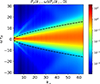Fig. A.1. Normalized velocity spectrum Pu(k⊥,  ω)/Pu(k⊥,  0) compared to the theoretical prediction for critically balanced turbulence ωCB ∼ k⊥2/3 (dashed black line).

All Figures

	Fig. 1. Temporal evolution of magnetic and kinetic energy variations ΔEmag and ΔEkin. The green shaded area represents the time interval used to calculate wavenumber-frequency spectra.
In the text

	Fig. 2. (k∥,  ω) and (k⊥,  ω) projections of PB (a)–(b), Pρ (c)–(d), Pui (e)–(f), and Puc (g)–(h). The dashed lines indicate dispersion relations of Alfvén waves (AW) and slow modes (SM) for k⊥ = 0, and fast modes (FM) for k∥ = 0.
In the text

	Fig. 3. Frequency spectra of u, ui, and uc at (k⊥ = 1,  k∥ = 10) (a), (k⊥ = 25,  k∥ = 5) (b), and (k⊥ = 8,  k∥ = 8) (c). The vertical dashed lines indicate the corresponding frequencies of Alfvén waves (blue), slow modes (black), and fast modes (red).
In the text

	Fig. A.1. Normalized velocity spectrum Pu(k⊥,  ω)/Pu(k⊥,  0) compared to the theoretical prediction for critically balanced turbulence ωCB ∼ k⊥2/3 (dashed black line).
In the text

References

- Adhikari, L., Zank, G. P., & Zhao, L.-L. 2020, ApJ, 901, 102 [Google Scholar]
- Adhikari, L., Zank, G. P., Telloni, D., & Zhao, L.-L. 2022, ApJ, 937, L29 [NASA ADS] [CrossRef] [Google Scholar]
- Adhikari, L., Zank, G. P., Zhao, L., et al. 2024, ApJ, 965, 94 [Google Scholar]
- Adhikari, S., Yang, Y., & Matthaeus, W. H. 2025, Phys. Plasmas, submitted [arXiv:2503.11825] [Google Scholar]
- Arrò, G., Califano, F., & Lapenta, G. 2022, A&A, 668, A33 [NASA ADS] [CrossRef] [EDP Sciences] [Google Scholar]
- Arrò, G., Pucci, F., Califano, F., Innocenti, M. E., & Lapenta, G. 2023, ApJ, 958, 11 [Google Scholar]
- Arrò, G., Califano, F., Pucci, F., Karlsson, T., & Li, H. 2024, ApJ, 970, L6 [Google Scholar]
- Arrò, G., Li, H., & Matthaeus, W. H. 2025, PRL, 134, 235201 [Google Scholar]
- Bhatia, H., Norgard, G., Pascucci, V., & Bremer, P.-T. 2012, IEEE TVCG, 19, 1386 [Google Scholar]
- Bhattacharjee, A., Ng, C., & Spangler, S. 1998, ApJ, 494, 409 [Google Scholar]
- Cerri, S. S., Califano, F., Jenko, F., Told, D., & Rincon, F. 2016, ApJ, 822, L12 [NASA ADS] [CrossRef] [Google Scholar]
- Cerri, S. S., Arzamasskiy, L., & Kunz, M. W. 2021, ApJ, 916, 120 [NASA ADS] [CrossRef] [Google Scholar]
- Chandran, B. D., & Perez, J. C. 2019, JPP, 85, 905850409 [Google Scholar]
- Cho, J., & Lazarian, A. 2002, PRL, 88, 245001 [Google Scholar]
- Cho, J., & Lazarian, A. 2003, MNRAS, 345, 325 [NASA ADS] [CrossRef] [Google Scholar]
- Cranmer, S. R., Gibson, S. E., & Riley, P. 2017, SSR, 212, 1345 [Google Scholar]
- Espinoza-Troni, J., Arrò, G., Asenjo, F. A., & Moya, P. S. 2025, ApJ, 986, 228 [Google Scholar]
- Gan, Z., Li, H., Fu, X., & Du, S. 2022, ApJ, 926, 222 [NASA ADS] [CrossRef] [Google Scholar]
- Goldreich, P., & Sridhar, S. 1995, ApJ, 438, 763 [Google Scholar]
- Hadid, L., Sahraoui, F., & Galtier, S. 2017, ApJ, 838, 9 [NASA ADS] [CrossRef] [Google Scholar]
- Horbury, T. S., Forman, M., & Oughton, S. 2008, PRL, 101, 175005 [Google Scholar]
- Howes, G., Bale, S., Klein, K., et al. 2012, ApJ, 753, L19 [NASA ADS] [CrossRef] [Google Scholar]
- Hunana, P., & Zank, G. 2010, ApJ, 718, 148 [Google Scholar]
- Karimabadi, H., Roytershteyn, V., Wan, M., et al. 2013, PoP, 20 [Google Scholar]
- Kasper, J., Klein, K., Lichko, E., et al. 2021, PRL, 127, 255101 [Google Scholar]
- Klein, K., Howes, G., TenBarge, J., et al. 2012, ApJ, 755, 159 [NASA ADS] [CrossRef] [Google Scholar]
- Kreiss, H.-O. 1980, CPAM, 33, 399 [Google Scholar]
- Li, H., Gary, S. P., & Stawicki, O. 2001, GRL, 28, 1347 [Google Scholar]
- Lugones, R., Dmitruk, P., Mininni, P. D., Pouquet, A., & Matthaeus, W. H. 2019, PoP, 26, 12 [Google Scholar]
- Matthaeus, W. H., & Brown, M. 1988, PF, 31, 3634 [Google Scholar]
- Matthaeus, W. H., Goldstein, M. L., & Roberts, D. A. 1990, JGR, 95, 20673 [Google Scholar]
- Matthaeus, W. H., Klein, L. W., Ghosh, S., & Brown, M. R. 1991, JGR, 96, 5421 [Google Scholar]
- Montgomery, D., Brown, M. R., & Matthaeus, W. 1987, JGR, 92, 282 [Google Scholar]
- Narita, Y., & Marsch, E. 2015, ApJ, 805, 24 [NASA ADS] [CrossRef] [Google Scholar]
- Papini, E., Cicone, A., Franci, L., et al. 2021, ApJ, 917, L12 [Google Scholar]
- Perrone, D., Alexandrova, O., Mangeney, A., et al. 2016, ApJ, 826, 196 [NASA ADS] [CrossRef] [Google Scholar]
- Pezzi, O., Malara, F., Servidio, S., et al. 2017, Phys. Rev. E, 96, 023201 [NASA ADS] [CrossRef] [Google Scholar]
- Pezzini, L., Zhukov, A. N., Bacchini, F., et al. 2024, ApJ, 975, 37 [NASA ADS] [CrossRef] [Google Scholar]
- Pezzini, L., Bacchini, F., Zhukov, A. N., Arrò, G., & Lopez, R. A. 2026, ApJ, 997, 158 [Google Scholar]
- Roberts, D., Klein, L., Goldstein, M., & Matthaeus, W. 1987, JGR, 92, 11021 [Google Scholar]
- Roberts, O., Narita, Y., Li, X., Escoubet, C., & Laakso, H. 2017, JGR, 122, 6940 [Google Scholar]
- Schekochihin, A., Cowley, S. C., Dorland, W., et al. 2009, ApJSS, 182, 310 [Google Scholar]
- Shebalin, J. V., Matthaeus, W. H., & Montgomery, D. 1983, JPP, 29, 525 [Google Scholar]
- Squire, J., Meyrand, R., Kunz, M. W., et al. 2022, NA, 6, 715 [Google Scholar]
- Stone, J. M., Tomida, K., White, C. J., & Felker, K. G. 2020, ApJSS, 249, 4 [Google Scholar]
- TenBarge, J., & Howes, G. 2012, PoP, 19, 5 [Google Scholar]
- TenBarge, J., Howes, G. G., Dorland, W., & Hammett, G. W. 2014, CPC, 185, 578 [Google Scholar]
- Verdini, A., Velli, M., & Buchlin, E. 2009, ApJ, 700, L39 [NASA ADS] [CrossRef] [Google Scholar]
- Verscharen, D., Chen, C. H., & Wicks, R. T. 2017, ApJ, 840, 106 [NASA ADS] [CrossRef] [Google Scholar]
- Verscharen, D., Chandran, B. D., Boella, E., et al. 2022, FASS, 9, 951628 [Google Scholar]
- Wicks, R., Horbury, T., Chen, C., & Schekochihin, A. 2010, MNRAS, 407, L31 [NASA ADS] [CrossRef] [Google Scholar]
- Yuen, K. H., Li, H., & Yan, H. 2025, ApJ, 986, 221 [Google Scholar]
- Zank, G., & Matthaeus, W. 1992a, JPP, 48, 85 [Google Scholar]
- Zank, G., & Matthaeus, W. 1992b, JGR, 97, 17189 [Google Scholar]
- Zank, G. P., & Matthaeus, W. 1993, Phys. Fluids A, 5, 257 [Google Scholar]
- Zank, G., Adhikari, L., Hunana, P., et al. 2017, ApJ, 835, 147 [Google Scholar]
- Zank, G., Adhikari, L., Hunana, P., et al. 2018, ApJ, 854, 32 [NASA ADS] [CrossRef] [Google Scholar]
- Zank, G. P., Zhao, L.-L., Adhikari, L., et al. 2023, ApJSS, 268, 18 [Google Scholar]
- Zank, G. P., Zhao, L.-L., Adhikari, L., et al. 2024, ApJ, 966, 75 [NASA ADS] [CrossRef] [Google Scholar]
- Zhao, L.-L., Zank, G., Nakanotani, M., & Adhikari, L. 2023, ApJ, 944, 98 [Google Scholar]
- Zhao, L.-L., Silwal, A., Zhu, X., Li, H., & Zank, G. 2025, ApJ, 979, L4 [Google Scholar]
- Zhdankin, V. 2021, ApJ, 922, 172 [Google Scholar]
No density fluctuations are injected by our driver, they develop as a consequence of the turbulent cascade.
In the case of turbulence developing over a large-scale inhomogeneous background, the equation  is replaced by a more general incompressibility condition (see, e.g., Zank et al. 2017).
Equations (14)–(16) and (20)–(23) can be rewritten in dimensional units by setting ϵ = MA and by using the normalization described in Zank et al. (2017).
We specify that by “nearly incompressible” we mean that the velocity field is mostly solenoidal, with |uc|≪|ui|, even if density fluctuations can be considered to be relatively large, with δρrms/ρ0 ≃ 0.22.