Hunting for methanol in the water-rich, planet-forming disk around HL Tau

A. Soave; M. Leemker; S. Facchini; L. Maud; K. L. J. Rygl; L. Testi

doi:10.1051/0004-6361/202558485

Open Access

Issue		A&A Volume 708, April 2026


Article Number		A375
Number of page(s)		14
Section		Interstellar and circumstellar matter
DOI		https://doi.org/10.1051/0004-6361/202558485
Published online		24 April 2026

A&A, 708, A375 (2026)

Hunting for methanol in the water-rich, planet-forming disk around HL Tau

A. Soave¹^,2^★, M. Leemker³, S. Facchini³, L. Maud⁴, K. L. J. Rygl⁵ and L. Testi¹^,6

¹ Alma Mater Studiorum - Università di Bologna, Dipartimento di Fisica e Astronomia "Augusto Righi", Via Gobetti 93/2, 40129 Bologna, Italy
² INAF – Osservatorio di Astrofisica e Scienza dello Spazio, Via P. Gobetti 93/3, 40129 Bologna, Italy
³ Dipartimento di Fisica, Università degli Studi di Milano, Via Celoria 16, 20133 Milano, Italy
⁴ European Southern Observatory, Karl-Schwarzschild Str. 2, 85748 Garching bei München, Germany
⁵ INAF – Istituto di Radioastronomia & Italian ALMA Regional Centre, Via P. Gobetti 101, 40129 Bologna, Italy
⁶ INAF – Osservatorio Astrofisico di Arcetri, Largo E. Fermi 5, 50125 Firenze, Italy

^★ Corresponding author: This email address is being protected from spambots. You need JavaScript enabled to view it.

Received: 9 December 2025
Accepted: 20 February 2026

Abstract

Context. Methanol, the simplest complex organic molecule found in space, is considered a key compound for the formation of chemical species of prebiotic interest. Methanol detections in protoplanetary disks remain scarce, even though it is frequently detected in the material surrounding other young stellar objects (YSOs).

Aims. We investigated the presence of methanol in the protoplanetary disk around the HL Tau protostar, motivated by the detection of spatially resolved warm water emission.

Methods. Given the similar volatilities of methanol and water, thermally desorbed gas-phase methanol is expected to emit from the same region of the HL Tau disk where water vapor has been observed. Accordingly, we selected and imaged the most promising ALMA archival observations to search for rotational methanol lines.

Results. We find no methanol emission in the analyzed archival datasets. Assuming optically thin emission and local thermodynamic equilibrium (LTE), we derive stringent upper limits on the methanol column density for different excitation temperatures: <7.2 × 10¹⁴ cm⁻² at 100 K and <1.8 × 10¹⁵ cm⁻² at 200 K, assuming a circular emitting region with a radius of 17 au (~0.12"). Furthermore, we obtain a stringent upper limit on the methanol-to-water column density ratio (<0.55 × 10⁻³ at 100 K and <1.4 × 10⁻³ at 200 K), which is, on average, an order of magnitude lower than the values measured for other YSOs and Solar System comets.

Conclusions. We argue that the most likely explanation for the methanol nondetection in HL Tau is the presence of optically thick dust in the central region of the disk, which obscures part of the methanol emission. The upper limit on the methanol-to-water ratio in the HL Tau disk is at least an order of magnitude smaller than most clouds, YSOs, and comets, possibly due to radiative transfer and/or excitation effects, or to a different chemical evolution compared to the other sources.

Key words: astrochemistry / protoplanetary disks / stars: individual: HL Tau / ISM: molecules / submillimeter: planetary systems

© The Authors 2026

Open Access article, published by EDP Sciences, under the terms of the Creative Commons Attribution License (https://creativecommons.org/licenses/by/4.0), which permits unrestricted use, distribution, and reproduction in any medium, provided the original work is properly cited.

This article is published in open access under the Subscribe to Open model. This email address is being protected from spambots. You need JavaScript enabled to view it. to support open access publication.

1 Introduction

Formed inside the cold and dense environment of the interstellar medium (ISM), complex organic molecules (COMs) are species that contain both carbon and hydrogen with at least six atoms (Herbst & van Dishoeck 2009; Ceccarelli et al. 2023). Among them, methanol (CH₃OH), the simplest possible alcohol, is of great interest from a prebiotic point of view. Indeed, laboratory experiments show that photochemical reactions of UV-irradiated CH₃OH molecules can lead to the assembly of more complex organic compounds (Öberg et al. 2009; Fedoseev et al. 2016; Chuang et al. 2017). Emission lines tracing gas-phase methanol and absorption features tracing methanol ices, as well as other COMs, are commonly detected in a wide range of astrophysical sources, from molecular clouds in star-forming regions to class II young stellar objects (YSOs; Boogert et al. 2015; Chen et al. 2023; Jørgensen et al. 2020; Law et al. 2025; McClure et al. 2023; McGuire 2022; Pontoppidan et al. 2003; Öberg et al. 2023; Scibelli & Shirley 2020). With the revolutionary capabilities of the ALMA radiointerferometer, and following the first detection of methyl cyanide in the MWC 480 disk (CH₃CN; Öberg et al. 2015), COMs are now detected in protoplanetary disks. Nevertheless, despite being ubiquitously present in younger YSOs, gas-phase CH₃OH remains an elusive species, detected in only seven protoplanetary disks to date (Walsh et al. 2016; van't Hoff et al. 2018; van der Marel et al. 2021; Booth et al. 2021, 2023; Booth et al. 2025, 2026).

This low detection rate of gas-phase CH₃OH in protoplanetary disks can be attributed to the fact that the bulk of methanol is locked onto the icy surface of dust grains throughout most of the disk (Walsh et al. 2014) and thermally desorbs at the methanol snow line close to the protostar. The line marks the disk midplane location where temperatures reach the CH₃OH desorption temperature of ~120 K (Penteado et al. 2017; Minissale et al. 2022). Recent studies suggest that, at least for warmer protoplanetary disks around Herbig Ae/Be stars, the CH₃OH reservoir is inherited from the natal molecular cloud (Booth et al. 2021), where methanol forms efficiently on the surface of dust grains via hydrogenation of carbon monoxide (CO; Fuchs et al. 2009) and/or via radical-molecule H-atom abstraction reaction (Santos et al. 2022). Moreover, recent evidence from a few disks suggests that the bulk of ices is inherited from the earliest phases of star and planet formation without undergoing extensive chemical processing. Observations of freshly sublimated water, whose deuteration level is a sensitive tracer of chemical processing in ices, in the L1551 IRS5 class I source and the V883 Ori disk reveal isotopic ratios similar to those found in protostellar envelopes (Andreu et al. 2023; Tobin et al. 2023; Leemker et al. 2025). Because there is no efficient methanol gas-phase formation pathway, and disk temperatures are too high for CO to freeze out, the gas-phase CH₃OH must originate from the sublimation of these pristine ices (Garrod & Herbst 2006; Geppert et al. 2006).

Observationally, Walsh et al. (2016) detected CH₃OH for the first time in the TW Hya protoplanetary disk. Subsequent observations of methanol lines, supported by thermochemical modeling, indicate that nonthermal desorption processes, primarily photodesorption, release CH₃OH into the gas phase (Ilee et al. 2026). Methanol emission is also found in the V883 Ori protoplanetary disk, a YSO whose FU Orionis-type star is undergoing an accretion burst, shifting the water snow line out to ~80 au in the outer disk (van't Hoff et al. 2018; Lee et al. 2019; Leemker et al. 2021; Tobin et al. 2023; Lee et al. 2024; Jeong et al. 2025; Wang et al. 2025; Zeng et al. 2025). In this case, the molecules detected in the gas phase within the snow line are believed to directly trace the thermally sublimated ice coating the dust grains. Methanol is also found in several transition protoplanetary disks around Herbig stars: HD 100546 (Booth et al. 2021, 2024a; Evans et al. 2025), IRS 48 (van der Marel et al. 2021; Brunken et al. 2022; Booth et al. 2024b; Temmink et al. 2025), HD 169142 (Booth et al. 2023), HD 100453 (Booth et al. 2025, 2026), and CQ Tau (Booth et al. 2026). In these Herbig sources with CH₃OH detections, the desorption mechanism is thermal, driven by the high temperatures reached by the directly irradiated cavity walls and, possibly, by subsequent vertical cycling of the grains (van der Marel et al. 2021). Carney et al. (2019) and Yamato et al. (2024) also derived stringent upper limits on the methanol column density for the full disks around the Herbig stars HD 163296 and the MWC 480. Similarly, Podio et al. (2019) derived tight constraints on the methanol budget in the younger DG Tau A disk, which is still in a transitional stage between a class I and II YSOs.

To better constrain the chemical processing and evolution of the methanol budget in protoplanetary disks, it is often useful to compare its abundance to that of other closely related molecules, such as water (H₂O). This is the case because methanol and water have similar volatilities, with an approximate desorption temperature of 120 and 150 K, respectively (Penteado et al. 2017; Minissale et al. 2022). Methanol and water therefore sublimate into the gas phase from the icy surfaces of dust grains in the same disk region, and consequently their snow lines are close to one another. Moreover, the methanol-to-water column density ratio is a useful diagnostic of the degree of chemical processing after ice sublimation during the evolution of YSOs, from young, still deeply embedded protostars to class II disks. This ratio is predicted to decrease with time due to two effects: firstly, CH₃OH forms efficiently only on dust grain surfaces in the ISM, whereas other gas formation routes may be effective for water (van Dishoeck et al. 2013); secondly, methanol is photodissociated twice as fast as water (Heays et al. 2017).

Given the close relation between the desorption temperatures of methanol and water, protoplanetary disks where gas-phase water is detected could potentially show signs of methanol emission. The HL Tau protoplanetary disk is therefore a promising candidate for the search for methanol, due to the recent discovery of three spectrally and spatially resolved H₂O lines that emit primarily from within 17 au of the central star and are likely to trace warm water (Facchini et al. 2024; Leemker et al. 2026). HL Tau is a young protostar (≲ 1 Myr) located in the Taurus star-forming region at a distance of ~140 pc (Galli et al. 2018). Yen et al. (2019) estimated its mass to be 2.1 M_⊙ using dynamical measurements. The protoplanetary disk around HL Tau, which was the first to be imaged at high angular resolution with ALMA (ALMA Partnership 2015), is rich in substructures and shows a multitude of rings and gaps (Stephens et al. 2023). The HL Tau system is classified as a YSO in a transition phase between class I and class II, due to the ongoing interaction between the envelope and the protoplanetary disk, as also traced by the presence of a streamer and an accretion shock seen with S-bearing molecules (Yen et al. 2019; Garufi et al. 2022; Leemker et al. 2026).

In this paper, we present our analysis of ALMA archival observations to constrain the methanol budget in the HL Tau protoplanetary disk. We introduce the methods and the ALMA observations in Sect. 2. Sect. 3 details the methanol nondetections and the derived upper limits on the methanol column density. In Sect. 4, we benchmark the HL Tau methanol-to-water column density ratio with that measured for other YSOs and comets. We also compare the upper limit on the methanol abundance found in HL Tau with that measured in disks with CH₃OH detections, taking advantage of available DALI thermochemical models. Additionally, we search for possible correlations between the sulfur monoxide (SO)-to-methanol line flux ratio and stellar luminosity in protoplanetary disks. This study allows us to connect the organic budget and the chemical complexity of the disk with sulfur chemistry. Lastly, we summarize our conclusions in Sect. 5.

2 Observations

2.1 Dataset selection criteria

Due to its asymmetric three-dimensional geometric shape, the methanol molecule has access to a large number of possible rotational transitions at temperatures close to its desorption temperature of ~120 K. Thus, nearly every ALMA archival observation of HL Tau covers at least one methanol transition. We therefore selected only datasets covering CH₃OH transitions predicted to be bright, assuming local thermodynamic equilibrium (LTE) and optically thin emission.

Under these assumptions, it is possible to relate $N_{u}^{thin}$ $Mathematical equation: $N_{\rm{u}}^{{\rm{thin}}}$$ , the column density of the atoms or molecules excited in the upper energy level E_u, to S_v, the flux density integrated over a velocity range ΔV: $N_{u}^{thin} = \frac{4 π}{A_{ul} h c} \frac{S_{v} Δ V}{Ω} .$ $Mathematical equation: $N_{\rm{u}}^{{\rm{thin}}} = {{4\pi } \over {{A_{{\rm{ul}}}}hc}}{{{S_v}\Delta V} \over \Omega }.$$ (1)

Here, c is the speed of light, h is the Planck constant, v is the frequency, A_ul is the Einstein coefficient of the transition, and Ω is the solid angle subtended by the emitting area of the source. Applying the natural logarithm to both sides of the Boltzmann equation after inserting Eq. (1), yields $l n (\frac{N_{u}^{thin}}{g_{u}}) = \ln N_{T} - \ln Q (T_{ex}) - \frac{E_{u}}{k T_{ex}} .$ $Mathematical equation: $ln\left( {{{N_{\rm{u}}^{{\rm{thin}}}} \over {{g_{\rm{u}}}}}} \right) = \ln {N_{\rm{T}}} - \ln Q\left( {{T_{{\rm{ex}}}}} \right) - {{{E_{\rm{u}}}} \over {k{T_{{\rm{ex}}}}}}.$$ (2)

The expression above links the excitation temperature, T_ex, and the average column density of the emitting species, N_T, to the ratio between $N_{u}^{thin}$ $Mathematical equation: $N_{\rm{u}}^{{\rm{thin}}}$$ and the degeneracy of the upper energy level, g_u. Here, Q(T_ex) denotes the partition function of the considered atom or molecule, and k is the Boltzmann constant. Thus, the expected line flux S_vΔV can be estimated using the following expression, derived from combining Eqs. (1) and (2): $\begin{array}{l} S_{v} Δ V & = & \frac{h c Ω}{4 π} \frac{A_{ul} g_{u}}{Q (T_{ex})} N_{T} exp (- \frac{E_{u}}{k T_{ex}}) \\ \propto & \frac{A_{ul} g_{u}}{Q (T_{ex})} exp (- \frac{E_{u}}{k T_{ex}}) . \end{array}$ $Mathematical equation: $\matrix{{{S_v}\Delta V} \hfill & = \hfill & {{{hc\Omega } \over {4\pi }}{{{A_{{\rm{ul}}}}{g_{\rm{u}}}} \over {Q\left( {{T_{{\rm{ex}}}}} \right)}}{N_T}{\rm{exp}}\left( { - {{{E_{\rm{u}}}} \over {k{T_{{\rm{ex}}}}}}} \right)} \hfill \cr {} \hfill & \propto \hfill & {{{{A_{{\rm{ul}}}}{g_{\rm{u}}}} \over {Q\left( {{T_{{\rm{ex}}}}} \right)}}{\rm{exp}}\left( { - {{{E_{\rm{u}}}} \over {k{T_{{\rm{ex}}}}}}} \right).} \hfill \cr }$$ (3)

Applying Eq. (3) to the CH₃OH line list from the CDMS database (Müller et al. 2001, 2005; Endres et al. 2016; Xu et al. 2008), we ranked all methanol rotational transitions within the 70–700 GHz frequency interval according to their expected line strength for an assumed T_ex = 150 K. We chose this value as a representative value T_ex for methanol based on that computed for the thermally desorbed CH₃OH reservoir in the HD 100546 disk (Evans et al. 2025) and on the temperature derived from the two water transitions with the lowest E_u in HL Tau (Facchini et al. 2024).

To identify the best observational programs for methanol detection, taking into account at the same time both the intrinsic properties of the molecular transitions and the technical features of the observation, we employed built-in methods from the Alminer library (Ahmadi & Hacar 2023) to cross-correlate the ranked CH₃OH line list with the ALMA archive. We first gathered every HL Tau observation that covered at least one methanol transition, rejecting those with coarse spectral (>5 km s⁻¹) or angular (>3″) resolution. These cut-offs were chosen to restrict our query only to frequency division mode (FDM) observations conducted with the 12-m array. The list of these CH₃OH lines was then ranked in decreasing order based on the ratio of the expected line flux, calculated using Eq. (3) and the line sensitivity of the observations. We selected all datasets covering at least one methanol transition with an estimated ratio within one third of the maximum value found for the lines in the 70–700 GHz interval. Table 1 summarizes the methanol lines (identified by their quantum numbers) that we imaged and analyzed. Three lines (7_(1,6)−7_(0,7) A, 9_(1,8)−9_(0,9) A, and 6_(1,5)−6_(0,6) A) were observed by more than one program.

Table 1

Relevant spectroscopic line properties of the targeted CH₃OH transitions, as well as the beam size, beam position angle (PA), and channel rms in the imaged line cubes.

2.2 Observations properties and line imaging

The dataset covering the selected CH₃OH lines belongs to Band 7 ALMA observations from three programs: 2017.1.01178.S (PI: E. Humphreys), 2022.1.00905.S (PI: S. Facchini), and 2019.1.00393.S (PI: K. Zhang). Detailed information on the observing set, calibrators, and spectral settings for each of these programs is presented in Appendix A. In Appendix B, we discuss the bandpass calibration of the observations from program 2022.1.00905.S, which are not thermal-noise limited but limited by spectral dynamical range.

We imaged the transitions in Table 1 using the CASA software package, version CASA 6.5.4-9 (CASA Team 2022). We began by subtracting the continuum emission of the HL Tau disk using the CASA task uvcontsub, fitting a first order polynomial after flagging channels covering bright lines. We then imaged each spectral window using tclean, setting the parameter niter to one. With no detectable methanol emission, we reconstructed dirty (niter = 0) cubes of all methanol lines in our sample, imaging 100 channels around the frequency of each CH₃OH transition. We chose a 1 km s⁻¹ channel spacing, close to the maximum velocity resolution allowed by the 976 kHz channel spectral windows (see Appendix A), without primary beam correction. We imaged the lines with Briggs weighting (Briggs 1995), setting the robust parameter to two to boost the sensitivity of the resulting data cubes at the expense of lower angular resolution. Because the B7 observations of program 2017.1.01178.S were taken at a very high angular resolution of 0.04″–0.08″, limiting the sensitivity to extended emission, we applied a 0.3″ uv-taper.

Table 1 reports the beam axes and the channel rms of the imaged line cubes. We evaluated the noise using the estimate_RMS function of the GoFish package (Teague 2019), which computes the line cube rms in a user-defined annular region. We used the first and last ten channels, as visual inspection of the data confirmed that they were line-free. We set the inner and outer radii to 3″ and 8″, respectively, to avoid including the emission from the disk.

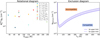Fig. 1

Left: rotational diagram built from the methanol nondetections. In the legend, each transition is labelled by its quantum numbers. For lines covered in multiple programs, the year of the program is also shown. Right: exclusion diagram showing excitation temperatures and total column densities compatible with the 3_σ and 5_σ upper limits on the total CH₃OH column density (the 3_σ limits are shown in the left panel).

2.3 Line stacking

We also stacked four CH₃OH lines from the 2017.1.01178.S program in the uv-plane: 6_(1.5)–6_(0.6) A, E_u = 63.71 K; 7_(1.6)–7(_0,7) A, E_u = 80.09 K; 9_(1,8)–9_(0,9) A, E_u = 119.88 K; and 10_(−0,10)−9_(−1,8) E, E_u = 140.60 K. Because stacking multiple lines in the frequency domain is not possible, the procedure first involved regridding the data with the CASA task cvel2 in velocity mode, assigning the systemic velocity of the system to the frequency of each line. We then concatenated the datasets into a single dataset and imaged it using the same parameters as described above, obtaining a channel rms of 1.18 mJy/beam. Because the two CH₃OH transitions in program 2019.1.00393.S (7_(1,7)−6_(1,6) A, E_u = 78.97 K; 12_(1,11)−12_(0,12) A, E_u = 197.08 K) belonged to the same spectral window, we also stacked these two lines together. The resulting data cube has an improved channel rms of 1.60 mJy/beam compared with individual values >2.2 mJy/beam.

3 Results

For each data cube covering the targeted methanol lines, we extracted spectra from a circular area centered on HL Tau with a radius of 0.7" using tools from the GoFish library. This mask corresponds to the spatial location of the H₂O emission in this disk (Facchini et al. 2024; Leemker et al. 2026). Figures F.1, F.2, and F.3 display the spectra of the lines covered in programs 2017.1.01178.S, 2022.1.00905.S, and 2019.1.00393.S, respectively. We detect no methanol emission in any of the 13 analyzed spectra. From this point onward, we exclude the stacked two data cubes from programs 2017.1.01178.S and 2019.1.00393.S, because the upper energy levels of the combined transitions differ by more than 60 K.

Following the methods of van't Hoff et al. (2020), when a line is not detected, it is still possible to derive the 3σ upper limit on $N_{u}^{thin}$ $Mathematical equation: $N_{\rm{u}}^{{\rm{thin}}}$$ from the spectrum rms (σ_spectrum), replacing S_vΔV in Eq. (1) with the the 3σ upper limit on the integrated line flux: $3 σ_{S_{v} Δ V} = 3 \times 1.1 \sqrt{Δ V δ V} \times σ_{spectrum} .$ $Mathematical equation: $3{\sigma _{{S_v}\Delta V}} = 3 \times 1.1\sqrt {\Delta V\delta V} \times {\sigma _{{\rm{spectrum}}}}.$$ (4)

Here, ΔV is the expected line width and δV is the spectral resolution, both in km s⁻¹. The 1.1 multiplicative factor accounts for the 10% uncertainty in the flux calibration of ALMA Band 7 (B7; Francis et al. 2020). In our analysis, we estimate σ_spectram as the mean of the rms in the spectra extracted from 50 random, nonoverlapping, emission-free circular regions of radius 0.7″. Table 2 reports the spectral noise estimated with this method.

To compute the 3σ upper limits on $N_{u}^{thin}$ $Mathematical equation: $N_{\rm{u}}^{{\rm{thin}}}$$ using Eqs. (1) and (4), we assumed a line width ΔV of 10 km s⁻¹, corresponding to the approximate width of the detected water line with the lowest E_u, and that the emitting area Ω is confined within the 17 au snow line constrained by Facchini et al. (2024). This assumption is motivated by the consideration that, if CH₃OH is thermally desorbed from the surface of dust grains in the disk, the main gas-phase methanol reservoir should be co-spatial with the water reservoir. The left panel of Fig. 1 shows how the upper limits $N_{u}^{thin}$ $Mathematical equation: $N_{\rm{u}}^{{\rm{thin}}}$$ , divided by g_u, vary with the E_u of each methanol transition in the rotational diagram. We note that a factor-of-two difference in the assumed ΔV would translate into a 40% difference in this upper limit. In contrast, an uncertainty of a factor of two in the radius of the circular emitting area Ω would result in a factor-of-four difference in $N_{u}^{thin}$ $Mathematical equation: $N_{\rm{u}}^{{\rm{thin}}}$$ ; this effect cancels out when computing the column density ratio with other molecules, because we assume that both molecules emit from the same region.

Since none of the imaged CH₃OH lines is detected, we computed the upper limits on the CH₃OH column density, $N_{{CH}_{3} OH}$ $Mathematical equation: ${N_{{\rm{C}}{{\rm{H}}_3}{\rm{OH}}}}$$ , following the procedure outlined in Goldsmith & Langer (1999) and assuming T_ex following Eq. (2). The right panel of Fig. 1 shows an exclusion diagram indicating the regions in the (T_ex, $N_{{CH}_{3} OH}$ $Mathematical equation: ${N_{{\rm{C}}{{\rm{H}}_3}{\rm{OH}}}}$$ ) parameter space compatible with the derived upper limits on the methanol column density. To create this figure, we combined the 3σ and 5σ upper limits on $N_{u}^{thin}$ $Mathematical equation: $N_{\rm{u}}^{{\rm{thin}}}$$ , varying the assumed excitation temperature from a nonphysical T_ex of 0–700 K, close to the maximum rotational temperature found by Facchini et al. (2024) for the three detected HL Tau water lines. For temperatures below 20 K, the exclusion diagram does not provide a meaningful constraint on the methanol column density, whereas at a temperature of ~38 K, it yields the lowest 3σ upper limit $(N_{{CH}_{3} OH} < 4.0 \times 10^{14} {cm}^{- 2})$ $Mathematical equation: $\left( {{N_{{\rm{C}}{{\rm{H}}_3}{\rm{OH}}}} < 4.0 \times {{10}^{14}}{\rm{c}}{{\rm{m}}^{ - 2}}} \right)$$ .

Table 2 reports the 3σ upper limits on N_T assuming three likely excitation temperatures for thermalized methanol emission. The true CH₃OH T_ex is expected to lie within the 100–200 K interval, based on the binding energy of CH₃OH to water ice (Penteado et al. 2017; Minissale et al. 2022) and the methanol excitation temperature measured via rotational diagram analysis in the HD 100453 and HD 100546 protoplanetary disks (Booth et al. 2025; Evans et al. 2025). Within this temperature interval, the 6_(1,5)–6_(0,6) A line from program 2022.1.00905.S provides the most stringent constraint on the methanol column density in the HL Tau disk, ranging from 7.2 × 10¹⁴ cm⁻² (T_ex = 100 K) − 1.8 × 10¹⁵ cm⁻² (T_ex=200 K).

These values are one to two orders of magnitude higher than the upper limit measured in the HL Tau disk by Garufi et al. (2021), using the 5_(0,5)−4_(0,4) A line at 241.79 GHz. This methanol transition is slightly colder (log₁₀A_ul = −4.22 and E_u = 34.81 K) than the 6_(1,5)−6_(0,6) A line (log₁₀A_ul = −3.47 and E_u = 63.71 K). The range of column density upper limits (1.9–7.5×10¹³ cm⁻²) was estimated assuming an excitation temperature of 20 K and 100 K, while an annular region with inner and outer radius of 55 and 250 au, respectively, was assumed for the methanol emitting area. Since $N_{{CH}_{3} OH}$ $Mathematical equation: ${N_{{\rm{C}}{{\rm{H}}_3}{\rm{OH}}}}$$ is inversely proportional to Ω, the difference between our values and those of Garufi et al. (2021) can be explained by our assumed emitting area (a circular region of radius 17 au), which is ~200 times smaller.

Table 2

Upper limits at the 3σ level on the disk-integrated CH₃OH flux and CH₃OH column density for various assumed excitation temperatures.

4 Discussion

4.1 Methanol-to-water column density ratio

From the collapse of a molecular cloud to the formation of a pro-toplanetary disk, the methanol budget remains closely tied to that of water due to their similar volatilities. Consequently, constraining the variation of the methanol-to-water column density ratio, both in the ices and in the gas phase, provides valuable insights into the degree of chemical processing that these two molecules undergo during the evolution of a YSO.

Figure 2 presents the CH₃OH/H₂O column density ratio measured for several clouds, YSOs, namely low- and high-mass YSOs (referred to as LYSOs and MYSOs, respectively), protoplanetary disks and Solar System comets, which are believed to be the remnants of the planet formation mechanisms that shaped our planetary system more than 4 Gyr ago (Oort 1950). This plot combines measurements obtained with different telescopes, targeting molecules in both the gas and ice phases. The values for molecular clouds, LYSOs, and MYSOs, measured by observing the ice absorption feature in the infrared (IR) spectra of background stars or of protostars themselves, are from Whittet et al. (2011) and references therein. We also used recent CH₃OH/H₂O ratios for two clouds and four LYSOs observed with JWST (McClure et al. 2023; Chen et al. 2024; Rocha et al. 2024, 2025). For LYSOs, radio-interferometric observations of gas-phase CH₃OH and $H_{2}^{18} O$ $Mathematical equation: ${\rm{H}}_2^{18}{\rm{O}}$$ yield column density ratios consistent with those found in the ices (Jensen et al. 2021; Jacobsen et al. 2019; Manigand et al. 2020; Persson et al. 2013; Okoda et al. 2024). The values for the comets, obtained with IR spectroscopy, are taken from the references listed in the review by Mumma & Charnley (2011), while the specific ratio for the 67P/Churyumov-Gerasimenko comet comes from the ROSINA mass spectrometer aboard the Rosetta spacecraft during an outgassing event of the comet near its perihelion (Rubin et al. 2019). Finally, we derived the values for the protoplanetary disks by combining gas-phase methanol column densities from the literature (see Table C.1, except for HL Tau) with water vapor column density measurements or upper limits also reported in the literature. The water column density upper limits for HD 100546 (Pirovano et al. 2022) and IRS 48 (Leemker et al. 2023) are based on Herschel far-IR data, whereas the values for V883 Ori (Tobin et al. 2023) and HL Tau (Facchini et al. 2024; Leemker et al. 2026) were measured at submillimeter wavelengths with ALMA. Water has also been detected in the DG Tau A protoplanetary disk in the far-IR with Herschel (Podio et al. 2013). We obtained the upper limit on the methanol-to-water ratio for this source by converting the total water vapor mass estimated from thermochemical modeling into a water column density and combining it with the methanol column density upper limit from Podio et al. (2019), scaled to the same emitting area. In the plot, we report three values for HL Tau, derived assuming a methanol excitation temperature of 100, 168, and 200 K and dividing by the water column density from Facchini et al. (2024) for an emitting area of ~ 17 au.

Assuming optically thin emission for all sources, Figure 2 shows how the CH₃OH/H₂O ratio varies over time. The ratio remains approximately constant for molecular clouds and class 0/1 YSOs still embedded in their collapsing envelopes, but it is on average a factor of five lower for Solar System comets.

Protoplanetary disks present a different picture: the five sources with measurements or upper limits display a large scatter, spanning more than five orders of magnitude. The V883 Ori disk is the only source with a methanol-to-water ratio consistent with clouds, LYSOs, and MYSOs. In this source, the central protostar is undergoing an accretion burst, effectively shifting the water snow line in the outer disk. The emission of freshly sublimated water and methanol originates from an annular region, due to the highly optically thick dust that resides in the center of the disk and, possibly, to a depletion of COM abundances in the inner disk (Lee et al. 2019; Leemker et al. 2021; Tobin et al. 2023; Yamato et al. 2024). The similarity between the gas-phase methanol-to-water column density ratio measured in the V883 Ori disk and that observed in the ices of other YSOs further supports the conclusion that the bulk of the icy material is inherited by disks from the ISM, without undergoing extensive chemical reprocessing (Booth et al. 2021; Tobin et al. 2023; Leemker et al. 2025).

In contrast, the disk around the 1RS 48 stars displays a ratio approximately two orders of magnitude higher, suggesting a potential different chemical evolution compared to V883 Ori. The high CH₃OH/H₂O ratio (≳5; Leemker et al. 2023) in the 1RS 48 system may be partially explained by subthermal excitation of methanol, which invalidates the LTE assumption used to derive the CH₃OH column density (Temmink et al. 2025).

Moreover, 1RS 48 is a peculiar source, hosting a large, asym-mettical, crescent-shaped dust trap located at 60-80 au from the central star (van der Marel et al. 2013). Emission from several COMs and oxygen-bearing molecules associated with the thermal desorption of ice has been detected (van der Marel et al. 2021; Brunken et al. 2022; Leemker et al. 2023; Booth et al. 2024b). Therefore, the high CH₃OH/H₂O ratio may result from a different chemical composition of the ices in the trap, from other effects that alter the ratio once the two species sublimate into the gas phase, or from differences in the wavelength ranges of the probed water and methanol emission lines (van der Marel et al. 2021; Leemker et al. 2023). Similarly, the upper and lower limit for the DG Tau A and HD 100546 disks are derived, respectively, from H₂O observations with Herschel in the far-IR and CH₃OH observations with ALMA in the (sub-)millimeter range. For these three disks, the water column density was computed from thermochemical models.

In contrast, the CH₃OH/H₂O ratio in the HL Tau disk comes from ALMA radio-interferomettic observations at similar wavelengths, as in the case of the V883 Ori disk. This approach enables a direct comparison between the two disks in a similar region of the electromagnetic specttum. By combining the upper limit on the methanol column density reported in Table 2 with the water column density measured by Facchini et al. (2024), we find a methanol-to-water column density ratio upper limit for HL Tau (<0.55 × 10⁻³ at 100 K and <1.4 × 10⁻³ at 200 K) that is one order of magnitude lower than that measured for other YSOs and for most Solar System comets. This ratio can be explained by radiative transfer effects or by a chemical difference.

Focusing on the first scenario, we neglect the wavelength dependence of the dust opacity, since the methanol and water column densities were computed from lines with roughly the same frequency. Following the discussion in Isella et al. (2016) and Weaver et al. (2018), we consider the following possibilities:

Both the CH₃OH and H₂O emission are either optically thin or become optically thick below τ_dust = 1, while the dust remains optically thick. Only the line photons that escape are emitted from the disk layer where τ_dust ≲ 1. Because the same disk region is probed, we do not expect major changes in the CH₃OH/H₂O column density ratio due to radiative transfer effects.
Water is optically thick above the surface where the continuum becomes optically thick, while methanol remains optically thin. In this case, the water column density is underestimated not only because part of the H₂O reservoir is hidden by optically thick dust, but also because of the optical depth of the line itself and continuum oversubtraction. This effect would further reduce the methanol-to-water column density ratio.
The water and methanol emission is optically thick above the τ_dust = 1 surface, making the values for the column densities unrepresentative of the true CH₃OH and H₂O. To test whether the CH₃OH lines could be optically thick, we estimate the maximum emitting area that an optically thick methanol reservoir could have while still being undetected. Using the channel rms in kelvin for each line cube and assuming a methanol excitation temperature of ~120 K, we computed the 3σ upper limit on the maximum methanol emitting area $A_{{CH}_{3} OH}$ $Mathematical equation: ${A_{{\rm{C}}{{\rm{H}}_3}{\rm{OH}}}}$$ as $A_{{CH}_{3} OH} = (3 \cdot σ_{channel rms} / T_{e x})$ $Mathematical equation: ${A_{{\rm{C}}{{\rm{H}}_3}{\rm{OH}}}} = \left( {3 \cdot {\sigma _{{\rm{channel rms}}}}/{T_{ex}}} \right)$$ . A_beam, where A_beam is the beam area. The tightest constraint on $A_{{CH}_{3} OH}$ $Mathematical equation: ${A_{{\rm{C}}{{\rm{H}}_3}{\rm{OH}}}}$$ is given by the 6_(1,5)–6_(0,6) A line from program 2022.1.00905.S. To be both optically thick and undetected simultaneously, the methanol emission would need to originate from a circular region with a radius ≲ 1.2 au. Because this radius is four times smaller than the estimated location of the water snow line in the disk (~ 5 au), it is unlikely that the methanol emission is optically thick (Guerra-Alvarado et al. 2024).
If water is masing, the methanol-to-water column density ratio in HL Tau would be higher. This scenario could occur if the high H₂O energy levels are overpopulated relative to the LTE scenario, causing the water column density derived by Facchini et al. (2024) to overestimate the actual H₂O column density. Although masing cannot be completely excluded, Leemker et al. (2026) recently showed that water is likely only weakly masing in the HL Tau disk.

Instead, if we assume that the stringent upper limit on the methanol-to-water ratio represents the true methanol and water bulk abundance in the disk, we likely trace a chemical effect and/or methanol depletion. A decrease in this ratio during YSO evolution is expected if the molecules desorb into the gas phase after the bulk of the ice reservoir is inherited from the earliest phases of star and planet formation (Booth et al. 2021; Tobin et al. 2023; Leemker et al. 2025). Methanol forms efficiently on the surface of ISM dust grains and dissociates twice as fast as water, which, conversely, can also form in the gas if the temperature exceeds 300 K. Combining these mechanisms, the gas-phase CH₃OH/H₂O ratio is expected to remain constant or decrease over time. A similar effect would occur if the water emission in HL Tau arises from a wind associated with the CO-traced outflow (Bacciotti et al. 2025): both H₂O and CH₃OH would dissociate rapidly, but higher temperatures would reform H₂O directly in the gas phase.

In summary, we have described the radiative transfer and chemical effects that could explain the low upper limit on the methanol-to-water column density ratio in the HL Tau pro-toplanetary disk. Nevertheless, other explanations, such as an intrinsically low CH₃OH abundance, cannot be excluded.

Fig. 2

Methanol-to-water (CH₃OH/H₂O) column density ratios reported in the literature for a wide range of clouds, YSOs, and Solar System comets (see Sect. 4.1 for references). The values for molecular clouds, LYSOs, and MYSOs reflect the ice composition, whereas the ratios were measured in the gas-phase for protoplanetary disks and comets. Open symbols indicate protoplanetary disks in which the upper or lower limit on the methanol-to-water column density ratio was estimated by combining measurements taken at different wavelength ranges. Upward triangles for the HD 100546 and the IRS 48 disks indicate lower limits, whereas downward triangles for DG Tau A and HL Tau indicate upper limits. HL Tau values were obtained by dividing the 3σ upper limit on the $N_{{CH}_{3} OH}$ $Mathematical equation: ${N_{{\rm{C}}{{\rm{H}}_3}{\rm{OH}}}}$$ for the three assumed excitation temperatures in Table 2 by the water column density measured by Facchini et al. (2024).

4.2 Methanol budget in protoplanetary disks and the effect of optically thick dust

Comparing the stringent upper limit on the methanol column density in the HL Tau disk with measurements in other pro-toplanetary disks can shed light on why we did not detect CH₃OH in this source. In addition to disks with constraints on both methanol and water column densities, CH₃OH has been observed in the TW Hya, HD 169142, HD 100453, and CQ Tau disks, all of which are transition disks (Walsh et al. 2016; Booth et al. 2021; Booth et al. 2025, 2026). Table C.1 summarizes the mass and luminosity of stars hosted by disks with methanol detection, as well as the CH₃OH column density values corresponding to the given excitation temperatures. We also report the stellar parameters of HL Tau and the CH₃OH column density upper limit, obtained for an assumed excitation temperature of 168 K.

To account for differences in methanol emission across our sample - for example, due to variations in the emitting area – we adopted the CH₃OH abundance, defined as the ratio of methanol to hydrogen column densities, as a common quantity for comparison. Because most disks have methanol column densities derived assuming an emitting area confined within the snow line, we also computed the corresponding hydrogen column density within this region using thermochemical models. For this purpose, we used published DALI (Bruderer et al. 2009, 2012; Bruderer 2013) models of these systems to estimate the average hydrogen column density ( $N_{h}^{snow} = N_{H}^{snow} + 2 N_{H_{2}}^{snow}$ $Mathematical equation: $N_{\rm{h}}^{{\rm{snow}}} = N_{\rm{H}}^{{\rm{snow}}} + 2N_{{{\rm{H}}_2}}^{{\rm{snow}}}$$ ), present in both atomic and molecular form, within the gas inside the CH₃OH snow line (r_snow). The procedure used to estimate $N_{h}^{snow}$ $Mathematical equation: $N_{\rm{h}}^{{\rm{snow}}}$$ for each disk is described in Appendix C. For the HD 100453, CQ Tau, and DG Tau A disks, however, we could not determine the hydrogen column density within the snow line because no thermochemical model was available. Moreover, we excluded the TW Hya disk from our analysis because our assumption of thermally desorbed methanol does not apply to this source. In this case, the detected gas-phase methanol reservoir originates beyond the snow line, where thermal desorption is negligible, and it is most likely released from dust grain surfaces via photodesorption (Walsh et al. 2016; Ilee et al. 2026).

Using Fig. 3, we searched for trends between the $N_{{CH}_{3} OH} / N_{h}^{snow}$ $Mathematical equation: ${N_{{\rm{C}}{{\rm{H}}_3}{\rm{OH}}}}/N_{\rm{h}}^{{\rm{snow}}}$$ ratio and the properties of the disk region where the thermally sublimated methanol reservoir is expected to reside. We used the (sub-)millimeter continuum flux density (left panel) and the gas mass M_snow (right panel) as proxies for these properties, both computed within the snow line. The method used to derive M_snow from the DALI thermochemical models is described in Appendix C, while Appendix D lists the ALMA Band 7 archival programs used to integrate the continuum flux inside r_snow. All flux densities are scaled to a common distance of 140 pc.

In both panels of Fig. 3, HL Tau does not follow the trend of transition disks hosting Herbig stars, which exhibit a $N_{{CH}_{3} OH} / N_{h}^{snow}$ $Mathematical equation: ${N_{{\rm{C}}{{\rm{H}}_3}{\rm{OH}}}}/N_{\rm{h}}^{{\rm{snow}}}$$ ratio at least three orders of magnitude higher than the upper limit derived for HL Tau. The presence of a central cavity could explain why methanol and other COMs are detected in transition disks: stellar radiation directly irradiates and heats the inner edge of the cavity wall, releasing into the gas phase material previously locked in the icy mantles of dust grains. Moreover, inside the cavity, methanol emission is less severely obscured by dust.

The V883 Ori protoplanetary disk shows a $N_{{CH}_{3} OH} / N_{h}^{snow}$ $Mathematical equation: ${N_{{\rm{C}}{{\rm{H}}_3}{\rm{OH}}}}/N_{\rm{h}}^{{\rm{snow}}}$$ ratio similar to that of other transition disks but exhibits a much higher millimeter flux density and gas mass within the snow line. These values arise from the distinct thermal structure of the disk, which was heated by a recent accretion outburst of the central FU Orionis-type protostar, currently reaching a luminosity of ~200 L_⊙ (Pickering 1890; Furlan et al. 2016). As a consequence, the water snow line shifted outward to ~80 au from the star, effectively releasing icy material from dust grains within this radius (van't Hoff et al. 2018; Leemker et al. 2021; Tobin et al. 2023; Wang et al. 2025).

Conversely, according to r_snow estimated from the DALI thermochemical model, methanol in the HL Tau disk should be thermally desorbed only in the inner disk within ~4 au from the central star. Several multiwavelength studies show that, at a frequency of ~300 GHz, dust in HL Tau remains highly optically thick inside 60 au or 90 au, depending on the assumed grain porosity (Carrasco-González et al. 2019; Guerra-Alvarado et al. 2024; Ueda et al. 2025). Optically thick dust can have a dramatic effect on line emission (Isella et al. 2016; Weaver et al. 2018; De Simone et al. 2020), as shown for the V883 Ori protoplanetary disk, where methanol and water emission are not centtally peaked because the dust remains optically thick out to a radius of ~40 au (Cieza et al. 2016; Houge et al. 2024). Therefore, optically thick dust can alter line emission and thus the CH₃OH abundance derived from observations, possibly explaining the methanol nondetection in HL Tau. Nonetheless, differences in the chemical composition of the disks in our sample cannot be excluded. Longer wavelength (e.g., centimeter) observations can further help investigate the effect of dust attenuation on COM line emission at (sub-)millimeter wavelength (De Simone et al. 2020).

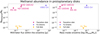Fig. 3

Ratio of methanol to average hydrogen column density versus Band 7 continuum flux integrated within the methanol snow line (left panel) and versus mass enclosed within r_snow (right panel). For the HL Tau disk, we show the 3σ upper limit on the $N_{{CH}_{3} OH}$ $Mathematical equation: ${N_{{\rm{C}}{{\rm{H}}_3}{\rm{OH}}}}$$ , assuming an excitation temperature of 168 K. The low methanol abundance upper limit in the HL Tau disk is likely due to differences in dust optical depth and stellar luminosity compared with other disks in our sample.

4.3 Sources with methanol and sulfur monoxide emission

Investigating the connection between sulfur and COM chemistry in protoplanetary disks can provide insight into the common condition that leads to sublimation of these species from ices. All protoplanetary disks with methanol detections also host gas-phase sulfur monoxide reservoirs, indicating shocks or sufficiently high temperatures to allow SO to desorb and/or form through gas-phase chemistry reactions (van Gelder et al. 2021). The latter is probably the case for HD 100546 (Booth et al. 2023; Booth et al. 2024a), HD 169142 (Booth et al. 2023; Law et al. 2023), HD 100453 (Booth et al. 2026), 1RS 48 (Booth et al. 2024b; Temmink et al. 2025), CQ Tau (Booth et al. 2026; Zagaria et al. 2025), and V883 Ori (Ruíz-Rodríguez et al. 2022). Additionally, in the disks around HD 100546 and HD 169142, SO could potentially trace the presence of an embedded planet. In all these sources, the CH₃OH and SO emission originates from a similar disk region enclosed within the water snow line. In TW Hya, however, the SO emission is asymmetric and localized in the southeast region of the disk, most likely due to an outflow driven by an embedded proto-planet in one of the gaps (Yoshida et al. 2024). Several sulfur monoxide lines have also been detected in the HL Tau system, tracing both the extended streamer seen in HCO⁺ and the accretion shock where the streamer impacts the disk (Garufi et al. 2022; Leemker et al. 2026). Moreover, higher-excitation SO transitions show that sulfur monoxide emission also originates from the inner disk of HL Tau, likely from SO molecules spiraling toward the star after being released from dust grains in the accretion shock. Similarly, volatile SO and SO₂ are released into the gas phase on the northwest side of the DG Tau A disk at the intersection with the streamer (Garufi et al. 2022).

To compare methanol and sulfur monoxide emission in disks where the two molecules present a similar spatial distribution, we followed the methodology described by Zagaria et al. (2025), rescaling both the integrated CH₃OH and SO line fluxes to the same ttansition and the same distance of 140 pc according to Eq. (E.1). The chosen reference lines are the J_N = 6₅−5₄ SO transition (as in Zagaria et al. 2025) and the 6_(1,5)−6_(0,6) A CH₃OH line because it provides the most stringent upper limit on the methanol column density in HL Tau. We assumed an LTE temperature of 50 K for SO, while for methanol we adopted the T_ex values listed in Table C.1 for each disk. For HL Tau, we considered the disk-integrated SO line flux from the high upper-energy level J_N = 15₁₅−14₁₄ transition presented in Garufi et al. (2022), since the emission mostly originates from the central part of the disk where CH₃OH should be thermally desorbed. Table E.1 lists the fluxes of the chosen methanol and sulfur monoxide transitions, as well their rescaled values for each disk. Due to the different morphology of the CH₃OH and SO emission in the disk, we did not include TW Hya in our analysis. The same consideration also applies to DG Tau A, where the SO emission originates from the northwest region of the disk, while the thermally desorbed methanol reservoir (which is not detected) is thought to reside in the inner disk.

Figure 4 shows how the methanol-to-sulfur monoxide flux ratio varies as a function of stellar luminosity for the disks in our sample. We do not observe correlation. Once again, the ratio for HL Tau is at least one order of magnitude lower than that in other protoplanetary disks, suggesting that the inner disk region where both chemical species are thermally desorbed from dust grains is depleted in gas-phase methanol. Another possible explanation is that the measured ratio for HL Tau reflects the chemical composition of the region where the streamer impacts the disk. Indeed, although the emission from the high-excitation SO transitions originates from the inner disk, the bulk of this volatile sulfur-bearing molecule reservoir likely comes from SO liberated by the accretion shock and then rapidly redistributed near the protostar. Because the estimated drifting timescale is shorter than the chemical reprocessing timescale required to alter the SO and SO₂ abundances set by the accretion shock (Garufi et al. 2022), the upper limit on the methanol-to-sulfur monoxide flux ratio in HL Tau would trace the chemical composition of the region where the streamer impacts the disk, under the assumption that also methanol is released into the gas phase by the shock and transported inward as SO.

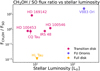Fig. 4

Methanol-to-sulfur monoxide line flux ratio versus stellar luminosity. The sample includes HL Tau, and all protoplanetary disks in which SO and CH₃OH are both detected and originate from a similar region of the disk enclosed within the water snow line.

5 Summary

In this work, we present an analysis of ALMA archival data of the HL Tau protoplanetary disk covering bright predicted methanol transitions. Our main findings are as follows:

We did not detect methanol in any of the datasets. Assuming that gas-phase methanol is thermalized and emitting within the water snow line, we derive the most stringent upper limit to date on the CH₃OH column density in this disk (<7.2 × 10¹⁴ cm⁻² at 100 K and < 1.8 × 10¹⁵ cm⁻² at 200 K). Furthermore, the low CH₃OH abundance compared with transition disks and V883 Ori suggests that the bulk of gas-phase methanol is hidden by optically thick dust in the HL Tau disk;
We computed the upper limit on the methanol-to-water column density ratio, finding values of <0.55 × 10⁻³ at 100 K and <1.4 × 10⁻³ at 200 K, which are an order of magnitude lower than those measured in other YSOs;
In the region where the streamer impacts the disk, the methanol-to-sulfur monoxide flux ratio in HL Tau is at least two orders of magnitude lower than that in other disks with CH₃OH detections;
We show that, when searching for weak lines on top of a bright continuum source, special care must be taken to optimize the signal-to-noise ratio per channel of the bandpass calibrator to avoid introducing noise into the scientific target.

Acknowledgements

We are grateful to the anonymous referee for the constructive comments and suggestions. We thank Luna Rampinelli for the useful discussions and Luke Keyte for sharing the HD 169142 disk model. This paper makes use of the following ALMA data: 2012.1.00799.S, 2013.1.00100.S, 2015.1.00806.S, 2016.1.00629.S, 2016.1.00728.S, 2017.1.01178.S, 2019.1.00393.S and 2022.1.00905.S. ALMA is a partnership of ESO (representing its member states), NSF (USA) and NINS (Japan), together with NRC (Canada), NSTC and ASIAA (Taiwan), and KASI (Republic of Korea), in cooperation with the Republic of Chile. The Joint ALMA Observatory is operated by ESO, AUI/NRAO and NAOJ. A.S. and LT work was partly supported by the Italian Ministero dell'Istruzione, Università e Ricerca through the grant Progetti Premiali 2012 – iALMA (CUP C52I13000140001). This project has received funding from the European Union's Horizon 2020 research and innovation programme through the European Research Council (ERC) ERC Synergy Grant ECOGAL (grant 855130). Views and opinions expressed are however those of the author(s) only and do not necessarily reflect those of the European Union or the European Research Council Executive Agency. Neither the European Union nor the granting authority can be held responsible for them. M.L. and S.F. are funded by the European Union (ERC, UNVEIL, 101076613). Views and opinions expressed are however those of the author(s) only and do not necessarily reflect those of the European Union or the European Research Council. Neither the European Union nor the granting authority can be held responsible for them. S.F. acknowledges financial contribution from PRIN-MUR 2022YP5ACE.

References

Ahmadi, A., & Hacar, A. 2023, ALminer: ALMA archive mining and visualization toolkit, Astrophysics Source Code Library [record ascl:2306.025] [Google Scholar]
ALMA Partnership (Brogan, C. L., et al.) 2015, ApJ, 808, L3 [Google Scholar]
Andreu, A., Coutens, A., Cruz-Sáenz de Miera, F., et al. 2023, A&A, 677, L17 [NASA ADS] [CrossRef] [EDP Sciences] [Google Scholar]
Bacciotti, F., Nony, T., Podio, L., et al. 2025, A&A, 704, A157 [NASA ADS] [CrossRef] [EDP Sciences] [Google Scholar]
Boogert, A. C. A., Gerakines, P. A., & Whittet, D. C. B. 2015, ARA&A, 53, 541 [Google Scholar]
Booth, A. S., Walsh, C., van Scheltinga, J. T., et al. 2021, Nat. Astron., 5, 684 [NASA ADS] [CrossRef] [Google Scholar]
Booth, A. S., Ilee, J. D., Walsh, C., et al. 2023, A&A, 669, A53 [Google Scholar]
Booth, A. S., Law, C. J., Temmink, M., Leemker, M., & Macias, E. 2023, A&A, 678, A146 [NASA ADS] [CrossRef] [EDP Sciences] [Google Scholar]
Booth, A. S., Leemker, M., van Dishoeck, E. F., et al. 2024a, AJ, 167, 164 [NASA ADS] [CrossRef] [Google Scholar]
Booth, A. S., Temmink, M., van Dishoeck, E. F., et al. 2024b, AJ, 167, 165 [NASA ADS] [CrossRef] [Google Scholar]
Booth, A. S., Wölfer, L., Temmink, M., et al. 2025, ApJ, 986, L9 [Google Scholar]
Booth, A. S., Calahan, J., Temmink, M., et al. 2026, AJ, 171, 128 [Google Scholar]
Briggs, D. S. 1995, PhD thesis, New Mexico Institute of Mining and Technology [Google Scholar]
Bruderer, S. 2013, A&A, 559, A46 [NASA ADS] [CrossRef] [EDP Sciences] [Google Scholar]
Bruderer, S., Doty, S. D., & Benz, A. O. 2009, ApJS, 183, 179 [Google Scholar]
Bruderer, S., van Dishoeck, E. F., Doty, S. D., & Herczeg, G. J. 2012, A&A, 541, A91 [NASA ADS] [CrossRef] [EDP Sciences] [Google Scholar]
Bruderer, S., van der Marel, N., van Dishoeck, E. F., & van Kempen, T. A. 2014, A&A, 562, A26 [NASA ADS] [CrossRef] [EDP Sciences] [Google Scholar]
Brunken, N. G. C., Booth, A. S., Leemker, M., et al. 2022, A&A, 659, A29 [NASA ADS] [CrossRef] [EDP Sciences] [Google Scholar]
Carney, M. T., Hogerheijde, M. R., Guzmán, V. V., et al. 2019, A&A, 623, A124 [NASA ADS] [CrossRef] [EDP Sciences] [Google Scholar]
Carrasco-González, C., Sierra, A., Flock, M., et al. 2019, ApJ, 883, 71 [Google Scholar]
CASA Team (Bean, B., et al.) 2022, PASP, 134, 114501 [NASA ADS] [CrossRef] [Google Scholar]
Ceccarelli, C., Codella, C., Balucani, N., et al. 2023, in Astronomical Society of the Pacific Conference Series, 534, Protostars and Planets VII, ed. S. Inutsuka, Y. Aikawa, T. Muto, K. Tomida, & M. Tamura, 379 [NASA ADS] [Google Scholar]
Chen, Y., van Gelder, M. L., Nazari, P., et al. 2023, A&A, 678, A137 [NASA ADS] [CrossRef] [EDP Sciences] [Google Scholar]
Chen, Y., Rocha, W. R. M., van Dishoeck, E. F., et al. 2024, A&A, 690, A205 [NASA ADS] [CrossRef] [EDP Sciences] [Google Scholar]
Chuang, K. J., Fedoseev, G., Qasim, D., et al. 2017, MNRAS, 467, 2552 [NASA ADS] [Google Scholar]
Cieza, L. A., Casassus, S., Tobin, J., et al. 2016, Nature, 535, 258 [Google Scholar]
De Simone, M., Ceccarelli, C., Codella, C., et al. 2020, ApJ, 896, L3 [NASA ADS] [CrossRef] [Google Scholar]
Endres, C. P., Schlemmer, S., Schilke, P., Stutzki, J., & Müller, H. S. 2016, J. Mol. Spectrosc., 327, 95 [NASA ADS] [CrossRef] [Google Scholar]
Evans, L., Booth, A. S., Walsh, C., et al. 2025, ApJ, 982, 62 [Google Scholar]
Facchini, S., Testi, L., Humphreys, E., et al. 2024, Nat. Astron., 8, 587 [Google Scholar]
Fedoseev, G., Chuang, K. J., van Dishoeck, E. F., Ioppolo, S., & Linnartz, H. 2016, MNRAS, 460, 4297 [Google Scholar]
Francis, L., & van der Marel, N. 2020, ApJ, 892, 111 [Google Scholar]
Francis, L., Johnstone, D., Herczeg, G., Hunter, T. R., & Harsono, D. 2020, AJ, 160, 270 [NASA ADS] [CrossRef] [Google Scholar]
Fuchs, G. W., Cuppen, H. M., Ioppolo, S., et al. 2009, A&A, 505, 629 [NASA ADS] [CrossRef] [EDP Sciences] [Google Scholar]
Furlan, E., Fischer, W. J., Ali, B., et al. 2016, ApJS, 224, 5 [Google Scholar]
Gaia Collaboration (Brown, A. G. A., et al.) 2021, A&A, 649, A1 [NASA ADS] [CrossRef] [EDP Sciences] [Google Scholar]
Galli, P. A. B., Loinard, L., Ortiz-Léon, G. N., et al. 2018, ApJ, 859, 33 [Google Scholar]
Garrod, R. T., & Herbst, E. 2006, A&A, 457, 927 [NASA ADS] [CrossRef] [EDP Sciences] [Google Scholar]
Garufi, A., Podio, L., Codella, C., et al. 2021, A&A, 645, A145 [EDP Sciences] [Google Scholar]
Garufi, A., Podio, L., Codella, C., et al. 2022, A&A, 658, A104 [CrossRef] [EDP Sciences] [Google Scholar]
Geppert, W. D., Hamberg, M., Thomas, R. D., et al. 2006, Faraday Discuss., 133, 177 [Google Scholar]
Goldsmith, P. F., & Langer, W. D. 1999, ApJ, 517, 209 [Google Scholar]
Guerra-Alvarado, O. M., Carrasco-González, C., Macías, E., et al. 2024, A&A, 686, A298 [NASA ADS] [CrossRef] [EDP Sciences] [Google Scholar]
Hartmann, L., Calvet, N., Gullbring, E., & D’Alessio, P. 1998, ApJ, 495, 385 [Google Scholar]
Heays, A. N., Bosman, A. D., & van Dishoeck, E. F. 2017, A&A, 602, A105 [NASA ADS] [CrossRef] [EDP Sciences] [Google Scholar]
Herbst, E., & van Dishoeck, E. F. 2009, ARA&A, 47, 427 [Google Scholar]
Houge, A., Macías, E., & Krijt, S. 2024, MNRAS, 527, 9668 [Google Scholar]
Ilee, J. D., Walsh, C., & Calahan, J. K. 2026, AJ, 171, 3 [Google Scholar]
Isella, A., Guidi, G., Testi, L., et al. 2016, Phys. Rev. Lett., 117, 251101 [NASA ADS] [CrossRef] [Google Scholar]
Jacobsen, S. K., Jørgensen, J. K., Di Francesco, J., et al. 2019, A&A, 629, A29 [NASA ADS] [CrossRef] [EDP Sciences] [Google Scholar]
Jensen, S. S., Jørgensen, J. K., Kristensen, L. E., et al. 2021, A&A, 650, A172 [EDP Sciences] [Google Scholar]
Jeong, J.-H., Lee, J.-E., Lee, S., et al. 2025, ApJS, 276, 49 [Google Scholar]
Jørgensen, J. K., Belloche, A., & Garrod, R. T. 2020, ARA&A, 58, 727 [Google Scholar]
Kama, M., Bruderer, S., van Dishoeck, E. F., et al. 2016, A&A, 592, A83 [NASA ADS] [CrossRef] [EDP Sciences] [Google Scholar]
Kepley, A. A., Tsutsumi, T., Brogan, C. L., et al. 2020, PASP, 132, 024505 [Google Scholar]
Keyte, L., Kama, M., Booth, A. S., et al. 2023, Nat. Astron., 7, 684 [NASA ADS] [CrossRef] [Google Scholar]
Keyte, L., Kama, M., Booth, A. S., Law, C. J., & Leemker, M. 2024, MNRAS, 534, 3576 [Google Scholar]
Law, C. J., Booth, A. S., & Öberg, K. I. 2023, ApJ, 952, L19 [NASA ADS] [CrossRef] [Google Scholar]
Law, C. J., Zhang, Q., Frommer, A. C., et al. 2025, ApJS, 276, 54 [Google Scholar]
Lee, J.-E., Lee, S., Baek, G., et al. 2019, Nat. Astron., 3, 314 [Google Scholar]
Lee, J.-E., Kim, C.-H., Lee, S., et al. 2024, ApJ, 966, 119 [NASA ADS] [CrossRef] [Google Scholar]
Leemker, M., van’t Hoff, M. L. R., Trapman, L., et al. 2021, A&A, 646, A3 [EDP Sciences] [Google Scholar]
Leemker, M., Booth, A. S., van Dishoeck, E. F., et al. 2023, A&A, 673, A7 [NASA ADS] [CrossRef] [EDP Sciences] [Google Scholar]
Leemker, M., Booth, A. S., van Dishoeck, E. F., Wölfer, L., & Dent, B. 2024, A&A, 687, A299 [NASA ADS] [CrossRef] [EDP Sciences] [Google Scholar]
Leemker, M., Tobin, J. J., Facchini, S., et al. 2025, Nat. Astron., 9, 1486 [Google Scholar]
Leemker, M., Facchini, S., Curone, P., et al. 2026, A&A, 705, A193 [NASA ADS] [CrossRef] [EDP Sciences] [Google Scholar]
Liu, Y., Henning, T., Carrasco-González, C., et al. 2017, A&A, 607, A74 [NASA ADS] [CrossRef] [EDP Sciences] [Google Scholar]
Lynden-Bell, D., & Pringle, J. E. 1974, MNRAS, 168, 603 [Google Scholar]
Macías, E., Espaillat, C. C., Osorio, M., et al. 2019, ApJ, 881, 159 [CrossRef] [Google Scholar]
Manigand, S., Jørgensen, J. K., Calcutt, H., et al. 2020, A&A, 635, A48 [NASA ADS] [CrossRef] [EDP Sciences] [Google Scholar]
McGuire, B. A. 2022, ApJS, 259, 30 [NASA ADS] [CrossRef] [Google Scholar]
McClure, M. K., Rocha, W. R. M., Pontoppidan, K. M., et al. 2023, Nat. Astron., 7, 431 [NASA ADS] [CrossRef] [Google Scholar]
Minissale, M., Aikawa, Y., Bergin, E., et al. 2022, ACS Earth Space Chem., 6, 597 [NASA ADS] [CrossRef] [Google Scholar]
Müller, H. S. P., Thorwirth, S., Roth, D. A., & Winnewisser, G. 2001, A&A, 370, L49 [Google Scholar]
Müller, H. S. P., Schlöder, F., Stutzki, J., & Winnewisser, G. 2005, J. Mol. Struct., 742, 215 [Google Scholar]
Mumma, M. J., & Charnley, S. B. 2011, ARA&A, 49, 471 [Google Scholar]
Öberg, K. I., Garrod, R. T., van Dishoeck, E. F., & Linnartz, H. 2009, A&A, 504, 891 [NASA ADS] [CrossRef] [EDP Sciences] [Google Scholar]
Öberg, K. I., Guzmán, V. V., Furuya, K., et al. 2015, Nature, 520, 198 [Google Scholar]
Öberg, K. I., Facchini, S., & Anderson, D. E. 2023, ARA&A, 61, 287 [Google Scholar]
Okoda, Y., Oya, Y., Sakai, N., et al. 2024, ApJ, 970, 28 [Google Scholar]
Oort, J. H. 1950, Bull. Astron. Inst. Netherlands, 11, 91 [NASA ADS] [Google Scholar]
Penteado, E. M., Walsh, C., & Cuppen, H. M. 2017, ApJ, 844, 71 [Google Scholar]
Persson, M. V., Jørgensen, J. K., & van Dishoeck, E. F. 2013, A&A, 549, L3 [NASA ADS] [CrossRef] [EDP Sciences] [Google Scholar]
Pickering, E. C. 1890, Ann. Harvard Coll. Observ., 18, 1 [Google Scholar]
Pineda, J. E., Szulágyi, J., Quanz, S. P., et al. 2019, ApJ, 871, 48 [Google Scholar]
Pirovano, L. M., Fedele, D., van Dishoeck, E. F., et al. 2022, A&A, 665, A45 [NASA ADS] [CrossRef] [EDP Sciences] [Google Scholar]
Podio, L., Kamp, I., Codella, C., et al. 2013, ApJ, 766, L5 [NASA ADS] [CrossRef] [Google Scholar]
Podio, L., Bacciotti, F., Fedele, D., et al. 2019, A&A, 623, L6 [NASA ADS] [CrossRef] [EDP Sciences] [Google Scholar]
Pontoppidan, K. M., Dartois, E., van Dishoeck, E. F., Thi, W.-F., & d’Hendecourt, L. 2003, A&A, 404, L17 [NASA ADS] [CrossRef] [EDP Sciences] [Google Scholar]
Rocha, W. R. M., van Dishoeck, E. F., Ressler, M. E., et al. 2024, A&A, 683, A124 [NASA ADS] [CrossRef] [EDP Sciences] [Google Scholar]
Rocha, W. R. M., McClure, M. K., Sturm, J. A., et al. 2025, A&A, 693, A288 [NASA ADS] [CrossRef] [EDP Sciences] [Google Scholar]
Rubin, M., Altwegg, K., Balsiger, H., et al. 2019, MNRAS, 489, 594 [Google Scholar]
Ruíz-Rodríguez, D. A., Williams, J. P., Kastner, J. H., et al. 2022, MNRAS, 515, 2646 [CrossRef] [Google Scholar]
Santos, J. C., Chuang, K.-J., Lamberts, T., et al. 2022, ApJ, 931, L33 [NASA ADS] [CrossRef] [Google Scholar]
Scibelli, S., & Shirley, Y. 2020, ApJ, 891, 73 [NASA ADS] [CrossRef] [Google Scholar]
Stephens, I. W., Lin, Z.-Y. D., Fernández-López, M., et al. 2023, Nature, 623, 705 [NASA ADS] [CrossRef] [Google Scholar]
Teague, R. 2019, J. Open Source Softw., 4, 1632 [NASA ADS] [CrossRef] [Google Scholar]
Temmink, M., Booth, A. S., Leemker, M., et al. 2025, A&A, 693, A101 [NASA ADS] [CrossRef] [EDP Sciences] [Google Scholar]
Tobin, J. J., van’t Hoff, M. L. R., Leemker, M., et al. 2023, Nature, 615, 227 [NASA ADS] [CrossRef] [Google Scholar]
Ueda, T., Andrews, S. M., Carrasco-González, C., et al. 2025, ApJ, 990, 183 [Google Scholar]
van der Marel, N., van Dishoeck, E. F., Bruderer, S., et al. 2013, Science, 340, 1199 [Google Scholar]
van der Marel, N., van Dishoeck, E. F., Bruderer, S., et al. 2016, A&A, 585, A58 [NASA ADS] [CrossRef] [EDP Sciences] [Google Scholar]
van der Marel, N., Booth, A. S., Leemker, M., van Dishoeck, E. F., & Ohashi, S. 2021, A&A, 651, L5 [NASA ADS] [CrossRef] [EDP Sciences] [Google Scholar]
van Dishoeck, E. F., Herbst, E., & Neufeld, D. A. 2013, Chem. Rev., 113, 9043 [Google Scholar]
van Gelder, M. L., Tabone, B., van Dishoeck, E. F., & Godard, B. 2021, A&A, 653, A159 [CrossRef] [EDP Sciences] [Google Scholar]
van ’t Hoff, M. L. R., Tobin, J. J., Trapman, L., et al. 2018, ApJ, 864, L23 [Google Scholar]
van’t Hoff, M. L. R., Harsono, D., Tobin, J. J., et al. 2020, ApJ, 901, 166 [Google Scholar]
Vioque, M., Oudmaijer, R. D., Baines, D., Mendigutía, I., & Pérez-Martínez, R. 2018, A&A, 620, A128 [NASA ADS] [CrossRef] [EDP Sciences] [Google Scholar]
Walsh, C., Millar, T. J., Nomura, H., et al. 2014, A&A, 563, A33 [NASA ADS] [CrossRef] [EDP Sciences] [Google Scholar]
Walsh, C., Loomis, R. A., Öberg, K. I., et al. 2016, ApJ, 823, L10 [NASA ADS] [CrossRef] [Google Scholar]
Wang, Y., Ormel, C. W., Mori, S., & Bai, X.-N. 2025, A&A, 696, A38 [NASA ADS] [CrossRef] [EDP Sciences] [Google Scholar]
Weaver, E., Isella, A., & Boehler, Y. 2018, ApJ, 853, 113 [Google Scholar]
Whittet, D. C. B., Cook, A. M., Herbst, E., Chiar, J. E., & Shenoy, S. S. 2011, ApJ, 742, 28 [Google Scholar]
Xu, L.-H., Fisher, J., Lees, R. M., et al. 2008, J. Mol. Spectrosc., 251, 305 [NASA ADS] [CrossRef] [Google Scholar]
Yamato, Y., Aikawa, Y., Guzmán, V. V., et al. 2024, ApJ, 974, 83 [Google Scholar]
Yen, H.-W., Gu, P.-G., Hirano, N., et al. 2019, ApJ, 880, 69 [NASA ADS] [CrossRef] [Google Scholar]
Yoshida, T. C., Nomura, H., Law, C. J., et al. 2024, ApJ, 971, L15 [Google Scholar]
Zagaria, F., Jiang, H., Cataldi, G., et al. 2025, ApJ, 989, 30 [Google Scholar]
Zeng, S., Jeong, J.-H., Oyama, T., et al. 2025, AJ, 170, 33 [Google Scholar]

Appendix A Calibration of the observations

The dataset covering the selected CH3OH lines belong to Band 7 ALMA observations from three programs: 2017.1.01178.S (PI: Humphreys, E.), 2022.1.00905.S (PI: Facchini, S.) and 2019.1.00393.S (PI: Zhang, K.). Within the program 2017.1.01178.S, HL Tau has been observed in four execution blocks, two of which being in Band 7. The first Band 7 execution block was observed on November 24, 2017, with an integration time of 34 minutes and with an array configuration of 49 antennas, whose baselines ranged from 92 m to 8.5 km. J0431+1731 was used for phase calibration, and J0538-4405 for bandpass and flux calibration. The second execution block was observed for 31 minutes on August 12, 2019. In this case, 48 antennas with a maximum separation of 3.6 km were employed. The phase calibration and the flux/bandpass calibration relied, respectively, on the sources J0440+1437 and J0519-4546. The chosen spectral set-up, consisting in four spectral windows (spws) in FDM mode, was similar for both observations. Three of the spws have 1920 channels with a width of 976 kHz (~ 0.9 km s¹), for a total 1.875 GHz bandwidth, while the other one was set to an higher spectral resolution of 244 kHz (~ 0.2 km s⁻¹).

Within the program 2022.1.00905.S, HL Tau has been targeted by 41/45 antennas during two execution blocks observed in October 12 (EB0) and 15 (EB1), 2022, for a total integration time of 100 minutes. The maximum baseline was of 500 m, providing a more moderate resolution of ~ 0.8″ when compared to those achieved by the other two programs. The spectral set-up consisted of two low resolution spws with a channel width of 976 kHz (~ 0.9 km s⁻¹), and in two high resolution spws with a channel width of 244 kHz (~ 0.2 km s⁻¹), for a bandwidth of, respectively, 1.875 and 0.469 GHz. J0423-0120 was used as flux and bandpass calibrator, while J0431+1731 was used for phase referencing. More specific information on the self-calibration performed combining together the B7 datasets from program 2017.1.01178.S and 2022.1.00905.S are included in Facchini et al. (2024).

Lastly, the two execution blocks from program 2019.1.00393.S took place on January 3 and on May 5, 2022, for a total integration time of 43 minutes. The array configuration was comprised of 38/39 antennas, with baselines ranging from 15 m to 782 m. Out of the six spws, three were configured with a high spectral resolution of 122 kHz (~ 0.1 km s⁻¹), while the channel width for the remaining ones was of 244 and 976 kHz. J0510+1800 was used for flux and bandpass calibration, while J0431+1731 was used for phase calibration.

Appendix B Calibration of program 2022.1.00905.S observations

In searching for weak lines in targets with strong continuum emission -such as is the case for the HL Tau protoplanetary disk - , ideally one would need to achieve a bandpass signal-to-noise-ratio (SNR) at least five times higher than the expected target SNR per channel. Otherwise the SNR of the bandpass will impose a spectral dynamic range limit, meaning that weak lines will not be detectable given the bandpass solution SNR with respect to the target source strength.

This issue is evident in the observations from program 2022.1.00905.S. To illustrate it, we first tcleaned HL Tau with a 2 km s⁻¹ channel spacing and with a robust parameter of 2. The auto-multithresh algorithm (Kepley et al. 2020) was used to clean down to a 3σ level. The image cube indicates a peak flux of ~ 0.8 Jy beam⁻¹ per channel with a noise of ~ 0.7 mJy beam⁻¹ per channel, i.e., a spectral SNR in the image of ~ 1100. Then we also tcleaned the bandpass calibrator using the same parameters, achieving a spectral SNR of ~ 2000 (given the peak flux of ~ 3 Jy beam⁻¹ per channel and a rms of ~ 1.5 mJy beam⁻¹ per channel), which is just two times higher than that of the science target when solving for the bandpass at the same spectral resolution. Likewise, the antenna based solutions are of the same ratio. This would effectively hide any weak line in the noise.

Figure B.1 illustrates how this limited dynamic range affects the broad band observations from program 2022.1.00905.S. It shows the integrated spectrum from the image cube extracted over a 1″ circular area centered on HL Tau for the same spectral window (spw) observed in the two execution blocks EB0 and EB1. The native pipeline reduction is set to achieve at least an antenna based SNR of 50 per channel, and in the case of the wide band 1.875 GHz spw we use, there is no channel averaging as each channel has an estimated 170 SNR. The moving average performed on the integrated spectra from the image cube highlights a flux variation of ~ 0.003 Jy, effectively hindering a robust detection of any weak line.

To boost the dynamical range, we performed a new bandpass calibration binning together 38 channels per solution, improving six times the previous reached bandpass signal-to-noise ratio per channel, which should be sufficient for the bandpass noise not to limit the target. However, as the attempted calibration with more channel binning does not remove the intrinsic bandpass features on the source spectra, we decided to resort for our analysis to the original standard ALMA pipeline calibration, motivated also by the little to no improvement in the HL Tau image cube noise. The only sure way to get better SNR on the bandpass is to try select brighter sources or observe it for longer. Of course this come with the acknowledgment that the observations will be a less efficient, but could be necessary for such difficult weak line searches. Nonetheless, when carefully inspecting the spectra from these 2022.1.00905.S. program datasets, we took into consideration the limited dynamic range, in order to avoid mistaking a weak line for an induced instrumental ripple.

Appendix C Computing N_h and M_snow from DALI thermochemical model

In this section we explain the procedure that we followed to compute the average hydrogen column density $N_{h}^{snow}$ $Mathematical equation: $N_{\rm{h}}^{{\rm{snow}}}$$ , present in both atomic and molecular form, and the gas mass M_snow inside the CH₃OH snow line r_snow. Firstly, we estimated r_snow as the midplane location where the dust temperature reaches the methanol desorption temperature ~ 120 K. Following the prescription from Lynden-Bell & Pringle (1974) and Hartmann et al. (1998), the radial gas surface density Σ(R) profile used for the disk models is given by the product between a power law and a negative, outer disk dominating exponential: $Σ (R) = Σ_{0} \times {(\frac{R}{R_{c}})}^{- γ} \times \exp [- {(\frac{R}{R_{c}})}^{2 - γ}] .$ $Mathematical equation: $\Sigma \left( R \right) = {\Sigma _0} \times {\left( {{R \over {{R_c}}}} \right)^{ - \gamma }} \times \exp \left[ { - {{\left( {{R \over {{R_{\rm{c}}}}}} \right)}^{2 - \gamma }}} \right].$$ (C.1)

In the expression above, Σ₀ is the surface density at the characteristic radius R_c, while γ is the power law index. To account for the central cavity of the transitional disks in our sample, we multiplied the surface density in Eq. C.1 by the δ_gas parameter, which describes the relative drop in gas density inside the central gap, up to the outer radius of the gas cavity R_gas,cav. We have used a secondary δ_gas of 10⁻² and 10⁻³ when integrating 2 between R_gas,cav and the outer radius of the dust cavity R_dust,cav for, respectively, the HD 100546 and HD 169142 disks following the models presented in Leemker et al. (2024) and Keyte et al. (2024). For both of them, r_snow is locate between R_gas,cav and R_dust,cav. A summary of the relevant model parameters and references to the original works are presented in Table C.1, together with the computed values of r_snow and M_snow.

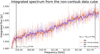Fig. B.1

Integrated spectrum from a 1″ circular region centered on HL Tau and extracted from the noncontinuum subtracted data cube. The orange and purple line differentiate the spectra extracted in two different execution blocks of the same spectral window. The bold lines were computed performing a moving average over ten consecutive channels to highlight the variations on a scale of ~ 0.003 Jy. The black dotted lines indicate the region of the spectrum where the two covered and nonde-tected methanol 3_(−1,2)−2_(−0,2) E and 6_(1,5)−6_(0,6) A line fall.

Table C.1

Relevant disk and stellar parameters of all disks with CH₃OH detections.

We estimate M_snow by integrating the surface density self-similar solution of a viscously evolving disk up to the snow line: $M_{snow} = \int_{0}^{2 π} \int_{0}^{r_{snow}} R Σ (R) d R d ϕ = 2 π m_{p} \int_{0}^{r_{snow}} R N (R) d R,$ $Mathematical equation: ${M_{{\rm{snow}}}} = \int_0^{2\pi } {\int_0^{{r_{{\rm{snow}}}}} {R\Sigma \left( R \right)dRd\phi = 2\pi {m_{\rm{p}}}} \int_0^{{r_{{\rm{snow}}}}} {RN\left( R \right)dR} } ,$$ (C.2)

where m_p is the mean mass of one particle in the DALI model (1.4 × 1.667 × 10⁻²⁴g), while N(R) is the gas column density.

Similarly, the average hydrogen column density within the snow line $N_{h}^{snow}$ $Mathematical equation: $N_{\rm{h}}^{{\rm{snow}}}$$ was computed as $N_{h}^{snow} = \frac{2 π \int_{0}^{r_{snow}} R N (R) d R}{π r_{snow}^{2}},$ $Mathematical equation: $N_{\rm{h}}^{{\rm{snow}}} = {{2\pi \int_0^{{r_{{\rm{snow}}}}} {RN\left( R \right)dR} } \over {\pi r_{{\rm{snow}}}^2}},$$ (C.3)

where N_h(R) is the hydrogen column density as a function of the radius.

Appendix D ALMA archival observation for the disk continuum flux

In order to compute the continuum flux density at ~300 GHz within the methanol snow line, we took available continuum product data from the ALMA archive, choosing for each disk B7 observations with good angular resolution (< 0.2″, in order to spatially resolve the snow line) and continuum sensitivity (< 0.06 mJy). The chosen programs from each disk are: HD 100546 (2015.1.00806.S; PI: Pineda, L; Pineda et al. 2019), HD 169142 (2012.1.00799.S; PI: Honda, M.; Macías et al. 2019), 1RS 48 (2013.1.00100.S; PI: van der Marel, N; van der Marel et al. 2016), V883 Ori (2016.1.00728.S; PI: Cieza, L.; Lee et al. 2019). For HL Tau we imaged the continuum from the datasets from program 2017.1.01178.S.

Table E.1

CH₃OH and SO line fluxes for the disks with methanol detections.

Appendix E CH₃OH and SO line fluxes

Table E.1 presents quantum numbers, frequencies, measured and rescaled fluxes for the CH₃OH and SO transitions that have been considered to compute the CH₃OH/SO line flux ratio shown in Fig. 4. Under the assumption of optically thin emission, we rescaled the observed line fluxes F_ohs to a common distance of 140 pc and to the the same transition, according to the following equation (Goldsmith & Langer 1999): $F_{ref} = F_{obs} \cdot {(\frac{distance}{140 pc})}^{2} \cdot \frac{A_{ul}^{ref} g_{ul}^{ref}}{A_{ul}^{obs} g_{ul}^{obs}} \cdot \exp (- \frac{(E_{u}^{ref} - E_{u}^{obs})}{k T_{ex}}) .$ $Mathematical equation: ${F_{{\rm{ref}}}} = {F_{{\rm{obs}}}} \cdot {\left( {{{{\rm{distance}}} \over {140{\rm{ pc}}}}} \right)^2} \cdot {{A_{{\rm{ul}}}^{{\rm{ref}}}g_{{\rm{ul}}}^{{\rm{ref}}}} \over {A_{{\rm{ul}}}^{{\rm{obs}}}g_{{\rm{ul}}}^{{\rm{obs}}}}} \cdot \exp \left( { - {{\left( {E_{\rm{u}}^{{\rm{ref}}} - E_{\rm{u}}^{{\rm{obs}}}} \right)} \over {k{T_{{\rm{ex}}}}}}} \right).$$ (E.1)

Appendix F CH₃OH integrated spectra

Figures F.1, F.2, and F.3 display, respectively, the spectra from the lines covered in the programs 2017.1.01178.S, 2022.1.00905.S, and 2019.1.00393.S. These are all integrated spectra extracted from a circular area centered on HL Tau with a radius of 0.7″.

Fig. F.1

Spectra extracted for all the CH₃OH lines covered inside the program 2017.1.01178.S

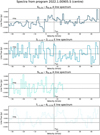Fig. F.2

Spectra extracted for all the CH₃OH lines covered inside the program 2022.1.00905.S.

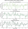Fig. F.3

Spectra extracted for all the CH₃OH lines covered inside the program 2019.1.00393.S.

All Tables

Table 1

Relevant spectroscopic line properties of the targeted CH₃OH transitions, as well as the beam size, beam position angle (PA), and channel rms in the imaged line cubes.

In the text

Table 2

Upper limits at the 3σ level on the disk-integrated CH₃OH flux and CH₃OH column density for various assumed excitation temperatures.

In the text

Table C.1

Relevant disk and stellar parameters of all disks with CH₃OH detections.

In the text

Table E.1

CH₃OH and SO line fluxes for the disks with methanol detections.

In the text

All Figures

	Fig. 4 Methanol-to-sulfur monoxide line flux ratio versus stellar luminosity. The sample includes HL Tau, and all protoplanetary disks in which SO and CH₃OH are both detected and originate from a similar region of the disk enclosed within the water snow line.
In the text

Fig. B.1

In the text

	Fig. F.1 Spectra extracted for all the CH₃OH lines covered inside the program 2017.1.01178.S
In the text

	Fig. F.2 Spectra extracted for all the CH₃OH lines covered inside the program 2022.1.00905.S.
In the text

	Fig. F.3 Spectra extracted for all the CH₃OH lines covered inside the program 2019.1.00393.S.
In the text

Current usage metrics show cumulative count of Article Views (full-text article views including HTML views, PDF and ePub downloads, according to the available data) and Abstracts Views on Vision4Press platform.

Data correspond to usage on the plateform after 2015. The current usage metrics is available 48-96 hours after online publication and is updated daily on week days.

Initial download of the metrics may take a while.

[R1] Ahmadi, A., & Hacar, A. 2023, ALminer: ALMA archive mining and visualization toolkit, Astrophysics Source Code Library [record ascl:2306.025] [Google Scholar]

[R2] ALMA Partnership (Brogan, C. L., et al.) 2015, ApJ, 808, L3 [Google Scholar]

[R3] Andreu, A., Coutens, A., Cruz-Sáenz de Miera, F., et al. 2023, A&A, 677, L17 [NASA ADS] [CrossRef] [EDP Sciences] [Google Scholar]

[R4] Bacciotti, F., Nony, T., Podio, L., et al. 2025, A&A, 704, A157 [NASA ADS] [CrossRef] [EDP Sciences] [Google Scholar]

[R5] Boogert, A. C. A., Gerakines, P. A., & Whittet, D. C. B. 2015, ARA&A, 53, 541 [Google Scholar]

[R6] Booth, A. S., Walsh, C., van Scheltinga, J. T., et al. 2021, Nat. Astron., 5, 684 [NASA ADS] [CrossRef] [Google Scholar]

[R7] Booth, A. S., Ilee, J. D., Walsh, C., et al. 2023, A&A, 669, A53 [Google Scholar]

[R8] Booth, A. S., Law, C. J., Temmink, M., Leemker, M., & Macias, E. 2023, A&A, 678, A146 [NASA ADS] [CrossRef] [EDP Sciences] [Google Scholar]

[R9] Booth, A. S., Leemker, M., van Dishoeck, E. F., et al. 2024a, AJ, 167, 164 [NASA ADS] [CrossRef] [Google Scholar]

[R10] Booth, A. S., Temmink, M., van Dishoeck, E. F., et al. 2024b, AJ, 167, 165 [NASA ADS] [CrossRef] [Google Scholar]

[R11] Booth, A. S., Wölfer, L., Temmink, M., et al. 2025, ApJ, 986, L9 [Google Scholar]

[R12] Booth, A. S., Calahan, J., Temmink, M., et al. 2026, AJ, 171, 128 [Google Scholar]

[R13] Briggs, D. S. 1995, PhD thesis, New Mexico Institute of Mining and Technology [Google Scholar]

[R14] Bruderer, S. 2013, A&A, 559, A46 [NASA ADS] [CrossRef] [EDP Sciences] [Google Scholar]

[R15] Bruderer, S., Doty, S. D., & Benz, A. O. 2009, ApJS, 183, 179 [Google Scholar]

[R16] Bruderer, S., van Dishoeck, E. F., Doty, S. D., & Herczeg, G. J. 2012, A&A, 541, A91 [NASA ADS] [CrossRef] [EDP Sciences] [Google Scholar]

[R17] Bruderer, S., van der Marel, N., van Dishoeck, E. F., & van Kempen, T. A. 2014, A&A, 562, A26 [NASA ADS] [CrossRef] [EDP Sciences] [Google Scholar]

[R18] Brunken, N. G. C., Booth, A. S., Leemker, M., et al. 2022, A&A, 659, A29 [NASA ADS] [CrossRef] [EDP Sciences] [Google Scholar]

[R19] Carney, M. T., Hogerheijde, M. R., Guzmán, V. V., et al. 2019, A&A, 623, A124 [NASA ADS] [CrossRef] [EDP Sciences] [Google Scholar]

[R20] Carrasco-González, C., Sierra, A., Flock, M., et al. 2019, ApJ, 883, 71 [Google Scholar]

[R21] CASA Team (Bean, B., et al.) 2022, PASP, 134, 114501 [NASA ADS] [CrossRef] [Google Scholar]

[R22] Ceccarelli, C., Codella, C., Balucani, N., et al. 2023, in Astronomical Society of the Pacific Conference Series, 534, Protostars and Planets VII, ed. S. Inutsuka, Y. Aikawa, T. Muto, K. Tomida, & M. Tamura, 379 [NASA ADS] [Google Scholar]

[R23] Chen, Y., van Gelder, M. L., Nazari, P., et al. 2023, A&A, 678, A137 [NASA ADS] [CrossRef] [EDP Sciences] [Google Scholar]

[R24] Chen, Y., Rocha, W. R. M., van Dishoeck, E. F., et al. 2024, A&A, 690, A205 [NASA ADS] [CrossRef] [EDP Sciences] [Google Scholar]

[R25] Chuang, K. J., Fedoseev, G., Qasim, D., et al. 2017, MNRAS, 467, 2552 [NASA ADS] [Google Scholar]

[R26] Cieza, L. A., Casassus, S., Tobin, J., et al. 2016, Nature, 535, 258 [Google Scholar]

[R27] De Simone, M., Ceccarelli, C., Codella, C., et al. 2020, ApJ, 896, L3 [NASA ADS] [CrossRef] [Google Scholar]

[R28] Endres, C. P., Schlemmer, S., Schilke, P., Stutzki, J., & Müller, H. S. 2016, J. Mol. Spectrosc., 327, 95 [NASA ADS] [CrossRef] [Google Scholar]

[R29] Evans, L., Booth, A. S., Walsh, C., et al. 2025, ApJ, 982, 62 [Google Scholar]

[R30] Facchini, S., Testi, L., Humphreys, E., et al. 2024, Nat. Astron., 8, 587 [Google Scholar]

[R31] Fedoseev, G., Chuang, K. J., van Dishoeck, E. F., Ioppolo, S., & Linnartz, H. 2016, MNRAS, 460, 4297 [Google Scholar]

[R32] Francis, L., & van der Marel, N. 2020, ApJ, 892, 111 [Google Scholar]

[R33] Francis, L., Johnstone, D., Herczeg, G., Hunter, T. R., & Harsono, D. 2020, AJ, 160, 270 [NASA ADS] [CrossRef] [Google Scholar]

[R34] Fuchs, G. W., Cuppen, H. M., Ioppolo, S., et al. 2009, A&A, 505, 629 [NASA ADS] [CrossRef] [EDP Sciences] [Google Scholar]

[R35] Furlan, E., Fischer, W. J., Ali, B., et al. 2016, ApJS, 224, 5 [Google Scholar]

[R36] Gaia Collaboration (Brown, A. G. A., et al.) 2021, A&A, 649, A1 [NASA ADS] [CrossRef] [EDP Sciences] [Google Scholar]

[R37] Galli, P. A. B., Loinard, L., Ortiz-Léon, G. N., et al. 2018, ApJ, 859, 33 [Google Scholar]

[R38] Garrod, R. T., & Herbst, E. 2006, A&A, 457, 927 [NASA ADS] [CrossRef] [EDP Sciences] [Google Scholar]

[R39] Garufi, A., Podio, L., Codella, C., et al. 2021, A&A, 645, A145 [EDP Sciences] [Google Scholar]

[R40] Garufi, A., Podio, L., Codella, C., et al. 2022, A&A, 658, A104 [CrossRef] [EDP Sciences] [Google Scholar]

[R41] Geppert, W. D., Hamberg, M., Thomas, R. D., et al. 2006, Faraday Discuss., 133, 177 [Google Scholar]

[R42] Goldsmith, P. F., & Langer, W. D. 1999, ApJ, 517, 209 [Google Scholar]

[R43] Guerra-Alvarado, O. M., Carrasco-González, C., Macías, E., et al. 2024, A&A, 686, A298 [NASA ADS] [CrossRef] [EDP Sciences] [Google Scholar]

[R44] Hartmann, L., Calvet, N., Gullbring, E., & D’Alessio, P. 1998, ApJ, 495, 385 [Google Scholar]

[R45] Heays, A. N., Bosman, A. D., & van Dishoeck, E. F. 2017, A&A, 602, A105 [NASA ADS] [CrossRef] [EDP Sciences] [Google Scholar]

[R46] Herbst, E., & van Dishoeck, E. F. 2009, ARA&A, 47, 427 [Google Scholar]

[R47] Houge, A., Macías, E., & Krijt, S. 2024, MNRAS, 527, 9668 [Google Scholar]

[R48] Ilee, J. D., Walsh, C., & Calahan, J. K. 2026, AJ, 171, 3 [Google Scholar]

[R49] Isella, A., Guidi, G., Testi, L., et al. 2016, Phys. Rev. Lett., 117, 251101 [NASA ADS] [CrossRef] [Google Scholar]

[R50] Jacobsen, S. K., Jørgensen, J. K., Di Francesco, J., et al. 2019, A&A, 629, A29 [NASA ADS] [CrossRef] [EDP Sciences] [Google Scholar]

[R51] Jensen, S. S., Jørgensen, J. K., Kristensen, L. E., et al. 2021, A&A, 650, A172 [EDP Sciences] [Google Scholar]

[R52] Jeong, J.-H., Lee, J.-E., Lee, S., et al. 2025, ApJS, 276, 49 [Google Scholar]

[R53] Jørgensen, J. K., Belloche, A., & Garrod, R. T. 2020, ARA&A, 58, 727 [Google Scholar]

[R54] Kama, M., Bruderer, S., van Dishoeck, E. F., et al. 2016, A&A, 592, A83 [NASA ADS] [CrossRef] [EDP Sciences] [Google Scholar]

[R55] Kepley, A. A., Tsutsumi, T., Brogan, C. L., et al. 2020, PASP, 132, 024505 [Google Scholar]

[R56] Keyte, L., Kama, M., Booth, A. S., et al. 2023, Nat. Astron., 7, 684 [NASA ADS] [CrossRef] [Google Scholar]

[R57] Keyte, L., Kama, M., Booth, A. S., Law, C. J., & Leemker, M. 2024, MNRAS, 534, 3576 [Google Scholar]

[R58] Law, C. J., Booth, A. S., & Öberg, K. I. 2023, ApJ, 952, L19 [NASA ADS] [CrossRef] [Google Scholar]

[R59] Law, C. J., Zhang, Q., Frommer, A. C., et al. 2025, ApJS, 276, 54 [Google Scholar]

[R60] Lee, J.-E., Lee, S., Baek, G., et al. 2019, Nat. Astron., 3, 314 [Google Scholar]

[R61] Lee, J.-E., Kim, C.-H., Lee, S., et al. 2024, ApJ, 966, 119 [NASA ADS] [CrossRef] [Google Scholar]

[R62] Leemker, M., van’t Hoff, M. L. R., Trapman, L., et al. 2021, A&A, 646, A3 [EDP Sciences] [Google Scholar]

[R63] Leemker, M., Booth, A. S., van Dishoeck, E. F., et al. 2023, A&A, 673, A7 [NASA ADS] [CrossRef] [EDP Sciences] [Google Scholar]

[R64] Leemker, M., Booth, A. S., van Dishoeck, E. F., Wölfer, L., & Dent, B. 2024, A&A, 687, A299 [NASA ADS] [CrossRef] [EDP Sciences] [Google Scholar]

[R65] Leemker, M., Tobin, J. J., Facchini, S., et al. 2025, Nat. Astron., 9, 1486 [Google Scholar]

[R66] Leemker, M., Facchini, S., Curone, P., et al. 2026, A&A, 705, A193 [NASA ADS] [CrossRef] [EDP Sciences] [Google Scholar]

[R67] Liu, Y., Henning, T., Carrasco-González, C., et al. 2017, A&A, 607, A74 [NASA ADS] [CrossRef] [EDP Sciences] [Google Scholar]

[R68] Lynden-Bell, D., & Pringle, J. E. 1974, MNRAS, 168, 603 [Google Scholar]

[R69] Macías, E., Espaillat, C. C., Osorio, M., et al. 2019, ApJ, 881, 159 [CrossRef] [Google Scholar]

[R70] Manigand, S., Jørgensen, J. K., Calcutt, H., et al. 2020, A&A, 635, A48 [NASA ADS] [CrossRef] [EDP Sciences] [Google Scholar]

[R71] McGuire, B. A. 2022, ApJS, 259, 30 [NASA ADS] [CrossRef] [Google Scholar]

[R72] McClure, M. K., Rocha, W. R. M., Pontoppidan, K. M., et al. 2023, Nat. Astron., 7, 431 [NASA ADS] [CrossRef] [Google Scholar]

[R73] Minissale, M., Aikawa, Y., Bergin, E., et al. 2022, ACS Earth Space Chem., 6, 597 [NASA ADS] [CrossRef] [Google Scholar]

[R74] Müller, H. S. P., Thorwirth, S., Roth, D. A., & Winnewisser, G. 2001, A&A, 370, L49 [Google Scholar]

[R75] Müller, H. S. P., Schlöder, F., Stutzki, J., & Winnewisser, G. 2005, J. Mol. Struct., 742, 215 [Google Scholar]

[R76] Mumma, M. J., & Charnley, S. B. 2011, ARA&A, 49, 471 [Google Scholar]

[R77] Öberg, K. I., Garrod, R. T., van Dishoeck, E. F., & Linnartz, H. 2009, A&A, 504, 891 [NASA ADS] [CrossRef] [EDP Sciences] [Google Scholar]

[R78] Öberg, K. I., Guzmán, V. V., Furuya, K., et al. 2015, Nature, 520, 198 [Google Scholar]

[R79] Öberg, K. I., Facchini, S., & Anderson, D. E. 2023, ARA&A, 61, 287 [Google Scholar]

[R80] Okoda, Y., Oya, Y., Sakai, N., et al. 2024, ApJ, 970, 28 [Google Scholar]

[R81] Oort, J. H. 1950, Bull. Astron. Inst. Netherlands, 11, 91 [NASA ADS] [Google Scholar]

[R82] Penteado, E. M., Walsh, C., & Cuppen, H. M. 2017, ApJ, 844, 71 [Google Scholar]

[R83] Persson, M. V., Jørgensen, J. K., & van Dishoeck, E. F. 2013, A&A, 549, L3 [NASA ADS] [CrossRef] [EDP Sciences] [Google Scholar]

[R84] Pickering, E. C. 1890, Ann. Harvard Coll. Observ., 18, 1 [Google Scholar]

[R85] Pineda, J. E., Szulágyi, J., Quanz, S. P., et al. 2019, ApJ, 871, 48 [Google Scholar]

[R86] Pirovano, L. M., Fedele, D., van Dishoeck, E. F., et al. 2022, A&A, 665, A45 [NASA ADS] [CrossRef] [EDP Sciences] [Google Scholar]

[R87] Podio, L., Kamp, I., Codella, C., et al. 2013, ApJ, 766, L5 [NASA ADS] [CrossRef] [Google Scholar]

[R88] Podio, L., Bacciotti, F., Fedele, D., et al. 2019, A&A, 623, L6 [NASA ADS] [CrossRef] [EDP Sciences] [Google Scholar]

[R89] Pontoppidan, K. M., Dartois, E., van Dishoeck, E. F., Thi, W.-F., & d’Hendecourt, L. 2003, A&A, 404, L17 [NASA ADS] [CrossRef] [EDP Sciences] [Google Scholar]

[R90] Rocha, W. R. M., van Dishoeck, E. F., Ressler, M. E., et al. 2024, A&A, 683, A124 [NASA ADS] [CrossRef] [EDP Sciences] [Google Scholar]

[R91] Rocha, W. R. M., McClure, M. K., Sturm, J. A., et al. 2025, A&A, 693, A288 [NASA ADS] [CrossRef] [EDP Sciences] [Google Scholar]

[R92] Rubin, M., Altwegg, K., Balsiger, H., et al. 2019, MNRAS, 489, 594 [Google Scholar]

[R93] Ruíz-Rodríguez, D. A., Williams, J. P., Kastner, J. H., et al. 2022, MNRAS, 515, 2646 [CrossRef] [Google Scholar]

[R94] Santos, J. C., Chuang, K.-J., Lamberts, T., et al. 2022, ApJ, 931, L33 [NASA ADS] [CrossRef] [Google Scholar]

[R95] Scibelli, S., & Shirley, Y. 2020, ApJ, 891, 73 [NASA ADS] [CrossRef] [Google Scholar]

[R96] Stephens, I. W., Lin, Z.-Y. D., Fernández-López, M., et al. 2023, Nature, 623, 705 [NASA ADS] [CrossRef] [Google Scholar]

[R97] Teague, R. 2019, J. Open Source Softw., 4, 1632 [NASA ADS] [CrossRef] [Google Scholar]

[R98] Temmink, M., Booth, A. S., Leemker, M., et al. 2025, A&A, 693, A101 [NASA ADS] [CrossRef] [EDP Sciences] [Google Scholar]

[R99] Tobin, J. J., van’t Hoff, M. L. R., Leemker, M., et al. 2023, Nature, 615, 227 [NASA ADS] [CrossRef] [Google Scholar]

[R100] Ueda, T., Andrews, S. M., Carrasco-González, C., et al. 2025, ApJ, 990, 183 [Google Scholar]

[R101] van der Marel, N., van Dishoeck, E. F., Bruderer, S., et al. 2013, Science, 340, 1199 [Google Scholar]

[R102] van der Marel, N., van Dishoeck, E. F., Bruderer, S., et al. 2016, A&A, 585, A58 [NASA ADS] [CrossRef] [EDP Sciences] [Google Scholar]

[R103] van der Marel, N., Booth, A. S., Leemker, M., van Dishoeck, E. F., & Ohashi, S. 2021, A&A, 651, L5 [NASA ADS] [CrossRef] [EDP Sciences] [Google Scholar]

[R104] van Dishoeck, E. F., Herbst, E., & Neufeld, D. A. 2013, Chem. Rev., 113, 9043 [Google Scholar]

[R105] van Gelder, M. L., Tabone, B., van Dishoeck, E. F., & Godard, B. 2021, A&A, 653, A159 [CrossRef] [EDP Sciences] [Google Scholar]

[R106] van ’t Hoff, M. L. R., Tobin, J. J., Trapman, L., et al. 2018, ApJ, 864, L23 [Google Scholar]

[R107] van’t Hoff, M. L. R., Harsono, D., Tobin, J. J., et al. 2020, ApJ, 901, 166 [Google Scholar]

[R108] Vioque, M., Oudmaijer, R. D., Baines, D., Mendigutía, I., & Pérez-Martínez, R. 2018, A&A, 620, A128 [NASA ADS] [CrossRef] [EDP Sciences] [Google Scholar]

[R109] Walsh, C., Millar, T. J., Nomura, H., et al. 2014, A&A, 563, A33 [NASA ADS] [CrossRef] [EDP Sciences] [Google Scholar]

[R110] Walsh, C., Loomis, R. A., Öberg, K. I., et al. 2016, ApJ, 823, L10 [NASA ADS] [CrossRef] [Google Scholar]

[R111] Wang, Y., Ormel, C. W., Mori, S., & Bai, X.-N. 2025, A&A, 696, A38 [NASA ADS] [CrossRef] [EDP Sciences] [Google Scholar]

[R112] Weaver, E., Isella, A., & Boehler, Y. 2018, ApJ, 853, 113 [Google Scholar]

[R113] Whittet, D. C. B., Cook, A. M., Herbst, E., Chiar, J. E., & Shenoy, S. S. 2011, ApJ, 742, 28 [Google Scholar]

[R114] Xu, L.-H., Fisher, J., Lees, R. M., et al. 2008, J. Mol. Spectrosc., 251, 305 [NASA ADS] [CrossRef] [Google Scholar]

[R115] Yamato, Y., Aikawa, Y., Guzmán, V. V., et al. 2024, ApJ, 974, 83 [Google Scholar]

[R116] Yen, H.-W., Gu, P.-G., Hirano, N., et al. 2019, ApJ, 880, 69 [NASA ADS] [CrossRef] [Google Scholar]

[R117] Yoshida, T. C., Nomura, H., Law, C. J., et al. 2024, ApJ, 971, L15 [Google Scholar]

[R118] Zagaria, F., Jiang, H., Cataldi, G., et al. 2025, ApJ, 989, 30 [Google Scholar]

[R119] Zeng, S., Jeong, J.-H., Oyama, T., et al. 2025, AJ, 170, 33 [Google Scholar]

Hunting for methanol in the water-rich, planet-forming disk around HL Tau

1 Introduction

2 Observations

2.1 Dataset selection criteria

2.2 Observations properties and line imaging

2.3 Line stacking

3 Results

4 Discussion

4.1 Methanol-to-water column density ratio

4.2 Methanol budget in protoplanetary disks and the effect of optically thick dust

4.3 Sources with methanol and sulfur monoxide emission

5 Summary

Acknowledgements

References

Appendix A Calibration of the observations

Appendix B Calibration of program 2022.1.00905.S observations

Appendix C Computing Nh and Msnow from DALI thermochemical model

Appendix D ALMA archival observation for the disk continuum flux

Appendix E CH3OH and SO line fluxes

Appendix F CH3OH integrated spectra

All Tables

All Figures

Appendix C Computing N_h and M_snow from DALI thermochemical model

Appendix E CH₃OH and SO line fluxes

Appendix F CH₃OH integrated spectra