| Issue |
A&A
Volume 708, April 2026
|
|
|---|---|---|
| Article Number | A228 | |
| Number of page(s) | 9 | |
| Section | Astronomical instrumentation | |
| DOI | https://doi.org/10.1051/0004-6361/202558573 | |
| Published online | 09 April 2026 | |
Field-dependent wavelength drift compensation in Fabry–Perot solar imaging spectrometers
1
Yunnan Observatories, Chinese Academy of Sciences,
Kunming
650216,
PR China
2
University of Chinese Academy of Sciences,
Beijing
100049,
PR China
3
Yunnan Key Laboratory of Solar Physics and Space Science,
Kunming
650216,
PR China
★ Corresponding author: This email address is being protected from spambots. You need JavaScript enabled to view it.
Received:
15
December
2025
Accepted:
9
March
2026
Abstract
Context. Fabry–Perot interferometers (FPIs) have become fundamental instruments for high-resolution imaging spectroscopy and magnetic field measurements in solar physics. In telecentric configurations, cavity defects of the FPI can introduce an inhomogeneous wavelength response across the field of view (FOV), which severely limits the accuracy of velocity and magnetic field diagnostics. Therefore, precise correction of the wavelength shift distribution is essential.
Aims. This study presents a method for compensating for the field-dependent wavelength drift of a telecentric air-gapped FPI instrument. The method allows for accurate calibration using data directly recorded by the instrument and provides precise measurements of wavelength shifts under actual observing conditions. This results in a reliable wavelength correction, which serves as a prerequisite for high-precision scientific observations.
Methods. The method scanned solar spectral lines directly through the scientific imaging path. Relative wavelength shifts across the FOV were then extracted using a cross-correlation algorithm combined with centroid localization. These shifts were decomposed into linear and nonlinear components. A response model linking actuator offset voltages to the linear drift slopes was constructed to actively compensate for the linear part, while the remaining nonlinear component is characterized as the intrinsic instrument bias.
Results. The method was applied to the Visible-light Imaging Spectrometer (VIS) at the New Vacuum Solar Telescope (NVST) of Yunnan Observatories. The voltage-to-slope response model demonstrated excellent performance, with R2 = 0.998 and root-mean-square error (RMSE) ≤0.007 V for both offset voltages, which enabled effective correction of the linear wavelength drift. After correction, the maximum wavelength shift decreased from 0.14 Å to 0.05 Å, significantly improving the homogeneity of the wavelength response and suppressing linear drift artifacts, thereby revealing previously obscured solar velocity signals. Moreover, a comparative analysis was conducted using the laser scanning technique, and showed excellent agreement with the results obtained from the proposed method.
Key words: instrumentation: interferometers / methods: observational / techniques: imaging spectroscopy
© The Authors 2026
 Open Access article, published by EDP Sciences, under the terms of the Creative Commons Attribution License (https://creativecommons.org/licenses/by/4.0), which permits unrestricted use, distribution, and reproduction in any medium, provided the original work is properly cited.
This article is published in open access under the Subscribe to Open model. This email address is being protected from spambots. You need JavaScript enabled to view it. to support open access publication.
1 Introduction
Fabry–Perot interferometers (FPIs) have become fundamental instruments for high-resolution solar observations due to their combination of high spectral resolution, large aperture, high transmittance, and rapid wavelength tuning capability. They are widely used for two-dimensional solar imaging spectroscopy and magnetic field measurements. Virtually all major ground-based solar telescopes are now equipped with air-gapped FPI instruments, such as the Visible-light Imaging Magnetograph (VIM) at the Goode Solar Telescope (Shumko et al. 2002; Denker et al. 2003), the CRisp Imaging SpectroPolarimeter (CRISP) at the Swedish Solar Telescope (Scharmer 2006; Scharmer et al. 2008), the Gregor Fabry–Perot Interferometer (GFPI) at the GREGOR telescope (Puschmann et al. 2012, 2013), and the Visible Tunable Filter (VTF) at the Daniel K. Inoue Solar Telescope (Kentischer et al. 2012; Schmidt et al. 2014). In spaceborne and balloon-borne applications, the lithium niobate FPI is typically adopted, such as the Polarimetric and Helioseismic Imager (PHI) on the Solar Orbiter mission (Solanki et al. 2020), the Imaging Magnetograph eXperiment (IMaX) on the Sunrise solar observatory (Martínez Pillet et al. 2011), and the Tunable Magnetograph (TuMag) for the SUNRISE III mission (del Toro Iniesta et al. 2025).
FPI instruments employ either collimated or telecentric configurations depending on their specific observational requirements. In the collimated configuration, the FPI is placed at a pupil plane, where a collimated beam from each field point illuminates the same etalon aperture. In the telecentric configuration, the FPI is positioned close to a focal plane. This placement causes each field point to generate a convergent beam of identical conic shape that illuminates only a small, local region of the etalon. The comparative merits and limitations of the two configurations are analyzed extensively in the literature (Beckers 1998; Scharmer 2006; Righini et al. 2010; Bailén et al. 2023). For the collimated setup, the transmission profile shifts toward a shorter wavelength as the incidence angle on the etalon increases, which produces a systematic blue shift across the field of view (FOV). A telecentric layout avoids such a phenomenon in principle and provides a homogeneous spectral response. In practice, this theoretical advantage is compromised of two main factors. First, limitations in the fabrication precision, coating uniformity, and plate parallelism of the etalon, along with residual assembly stress, often introduce spatial variations in the cavity spacing. These variations lead to etalon cavity defects (Halbgewachs et al. 2024), which are projected directly onto the image and produce field-dependent wavelength shifts. Second, the real instrument often departs from an ideal telecentric configuration, with the chief ray direction of each field point varying slightly. This variation produces a wavelength shift that depends on the local chief ray incidence angle on the etalon (Bailén et al. 2019). Collectively, these two types of error degrade spectral homogeneity; limit the accuracy of the vector velocity and magnetic field measurements derived from spectral profiles, Doppler shifts, and polarization states (Ruiz Cobo & del Toro Iniesta 1992; de la Cruz Rodríguez & van Noort 2017); and ultimately compromise the reliability of scientific results. To mitigate these errors, precise calibration of the field-dependent wavelength shift is required when the FPI is used in a telecentric configuration, which is essential for ensuring observational data quality and enabling accurate solar physical parameter measurements.
The laser scanning technique is widely used for characterizing cavity defects and calibrating the plate parallelism of the etalon (Denker & Tritschler 2005; Reardon & Cavallini 2008). This technique employs a dedicated calibration optical path in which a stabilized laser serves as the reference source. The laser beam is introduced into the etalon using a movable mirror. The cavity spacing is then tuned to scan the laser spectral profile. The shape and position of these profiles are then analyzed to quantify cavity defects and to derive the instrument transmission profile. As a mature calibration method, laser scanning provides a reliable foundation for correcting cavity defects. However, the increasing demands for data accuracy in solar physics require better consistency between calibration and scientific observing conditions. This has motivated the development of the calibration method that can be executed directly within the science imaging path. As a result, techniques that measure cavity defects directly from flat-field observations are now being implemented. Martínez Pillet et al. describe a method that uses flat-field data on IMaX to characterize the wavelength shift produced by the collimated configuration with a third-degree polynomial surface fit (Martínez Pillet et al. 2011). De la Cruz Rodríguez et al. implement an optimization scheme on CRISP that characterizes cavity defects by fitting the difference between the averaged spectrum and the observed spectrum from flat-field data (de la Cruz Rodríguez et al. 2015). Santamarina Guerrero et al. develop an optimization algorithm that uses analytical expressions of FPI transmission profiles for collimated and telecentric configurations. By comparing theoretical predictions with the measured data, they infer cavity defects from flat-field observations and apply the algorithm to PHI (Santamarina Guerrero et al. 2024). These approaches demonstrate that flat-field data play a critical role in the calibration of cavity defects and wavelength shift.
This paper presents a method for compensating field-dependent wavelength drift in telecentric air-gapped FPI instruments. The method builds on the flat-field calibration framework, operates without an auxiliary calibration path, and directly measures the wavelength shift under actual observing conditions. Based on these measurements, our method is employed to separate the linear wavelength drift arising from etalon non-parallelism. A dedicated correction model is then constructed to active compensate for this linear component effectively, thereby providing a more complete calibration solution for high-precision solar observations.
2 Field-dependent wavelength drift compensation principle
2.1 Wavelength shift measurement method
In an ideal telecentric configuration, each field point produces a convergent beam of identical shape, with its chief ray parallel to the optical axis. When an FPI is integrated into such a configuration, these chief rays enter the etalon perpendicularly and are subsequently imaged onto the detector. Consequently, there is a one-to-one mapping between a specific local region of the etalon cavity and each detector pixel, as shown in Fig. 1. The transmitted intensity at each pixel results from the coherent superposition of a cone of rays that reaches the etalon with a continuous angular distribution. The complete physical description of this process is relatively complex, involving electric field phase matching and analytical integration of the transmittance function, for which Bailén et al. (2021) first derived the rigorous analytical expressions. To concisely illustrate the principle of the proposed method, the Airy function (Born & Wolf 1999) was adopted as an approximate description for the transmitted intensity in a slow telecentric system. Accordingly, the transmitted intensity It(λ) detected at each pixel can be approximately expressed as
 (1)
(1)
where Ii denotes the incident intensity, R the plate reflectance, and A the absorptance. The phase difference δ is given by
 (2)
(2)
in which λ is the wavelength, h the cavity spacing, n the refractive index of medium inside the cavity (with n ≈ 1 for air), and θ the incidence angle (θ = 0 for normal incidence). When the phase difference satisfies δ = 2mπ, with m ∈ ℤ, the transmitted intensity reaches its maximum. Hence, for normal incidence and an air-gapped etalon, the central wavelength λ0 of the FPI transmission profile obeys
 (3)
(3)
with m representing the interference order.
The relationship between the central wavelength λ0 and the cavity spacing h for an ideal, defect-free etalon is given by Eq. (3). In reality, cavity defects introduce spatial variations in the cavity spacing, which can be described by a two-dimensional function h(x, y). This spatial inhomogeneity results in a variation of the central wavelength λ0(x, y) across the FOV. Since the local cavity spacing variation ∆h(x, y) = h(x, y) − h0 is sufficiently small compared to the nominal spacing h0, Eq. (3) can be differentiated to obtain a linear relationship between the wavelength shift ∆λ(x′, y′) measured at each pixel and the corresponding cavity defect ∆h(x, y). This relationship, expressed in Eq. (4), forms the theoretical foundation of the compensation method presented in this study. Based on it, the cavity defects are derived from the measured field-dependent wavelength drift, and the resulting linear wavelength drift is then compensated by adjusting the etalon parallelism:
 (4)
(4)
The wavelength shifts across the FOV are measured by analyzing the relative displacements of a solar spectral line from flat-field images. A quiet-Sun region near the disk center served as a calibration source, with the target spectral line sampled at regular wavelength intervals. To minimize the influence of intrinsic solar structural fluctuations, the telescope generates flat-field data by acquiring images in several random positions across the FOV. These data are used to construct a three-dimensional data cube (x′, y′, λ). From this cube, the spectral scanning profile  for each pixel and the mean spectrum of the entire field ⟨I(λ)⟩ are extracted. A cross-correlation algorithm combined with centroid localization is then applied to obtain the wavelength shifts between each pixel spectrum and the mean spectrum with the sub-pixel accuracy (Feng et al. 2012).
The spectrum of each pixel  and the mean spectrum ⟨I(λ)⟩ are first normalized to have zero mean and unit variance (Z-score normalization). This step removes large-scale intensity biases and emphasizes the relative shape of the spectral line profiles, which provides comparable morphological information for the subsequent cross-correlation analysis. The normalized spectra are then cross-correlated in the Fourier domain to compute the correlation function
  . The integer sampling-point position j0 at which the correlation reaches its maximum provides a coarse alignment. The corresponding peak correlation value,
  , serves as a quality metric for the spectral match, with values closer to 1 indicate higher reliability. To achieve sub-pixel accuracy, a local region centered on the correlation peak (position j0) is defined. After baseline subtraction and thresholding within this region, the centroid of the processed correlation values is calculated to obtain a fractional displacement jc that is finer than one sampling interval. Finally, these displacements are converted into the wavelength shifts according to
 (5)
(5)
where δλ is the spectral sampling interval (i.e., the wavelength difference between adjacent sampling points). This procedure produces a two-dimensional map of the wavelength shifts across the FOV with sub-pixel accuracy.
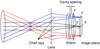 |
Fig. 1 Schematic diagram of the telecentric configuration. |
2.2 Offset voltage-to-linear drift slope response model
The field-dependent wavelength shift contains both linear and nonlinear components. The linear drift ∆λl originates mainly from nonparallelism between the etalon plates, manifesting as spatially linear wavelength variation across the FOV. The linear variation is modeled by the plane equation
 (6)
(6)
where (x′, y′) are the field coordinates centered on the FOV, a and b represent linear drift slopes along the x′ and y′ directions, reflecting the tilt of the etalon plate in the two directions, and c is a constant offset. Applying a least-squares fit of this plane to the measured wavelength shift map ∆λ(x′, y′) provides the optimal parameters a, b, and c. The fitting residual,
 (7)
(7)
defines the nonlinear shift, which arises from cavity defects that include substrate fabrication errors, coating nonuniformity, and assembly induced stress deformation.
The etalon is mounted on a three-point actuator support structure. Wavelength tuning is performed by applying a common differential voltage to all three actuators, while fine plate-tilt adjustments along the x and y directions are made by superposing independent offset voltages (Vx, Vy) on corresponding actuators. Consequently, the linear wavelength drift can be compensated by actively driving the actuators. To implement the compensation, a quantitative response model that links the actuator offset voltages to the linear drift slopes is established. A rotational misalignment may exist between the detector image axes (x′, y′) and the etalon physical axes (x, y). Therefore, applying an offset voltage along only one physical axis (x or y) can induce wavelength drift along both image axes (x′ and y′). To account for this coupling, two assumptions are made: a linear response between the offset voltages and the slopes, and a fixed rigid-body rotation between the two coordinate frames. Based on these assumptions, the required offset voltages (Vx, Vy) to produce the target drift slopes (a, b) are given by the affine transformation
![Mathematical equation: $\left[ {\matrix{{{V_x}} \cr {{V_y}} \cr } } \right] = \left[ {\matrix{A & B & E \cr C & D & F \cr } } \right]\left[ {\matrix{a \cr b \cr 1 \cr } } \right],$](/articles/aa/full_html/2026/04/aa58573-25/aa58573-25-eq12.png) (8)
(8)
where the matrix ![Mathematical equation: $\left[ {\matrix{ A & B & E \cr C & D & F \cr } } \right]$](/articles/aa/full_html/2026/04/aa58573-25/aa58573-25-eq13.png) is the control matrix that maps the slopes (a, b) to the required actuator offset voltages (Vx, Vy). The elements A, B, C, D represent the linear response sensitivities, which reflect the rotational and scaling coupling between the two coordinate systems, while E and F are the zero offset voltages needed when no drift is present a = 0, b = 0.
is the control matrix that maps the slopes (a, b) to the required actuator offset voltages (Vx, Vy). The elements A, B, C, D represent the linear response sensitivities, which reflect the rotational and scaling coupling between the two coordinate systems, while E and F are the zero offset voltages needed when no drift is present a = 0, b = 0.
To determine the control matrix, N predefined offset voltage pairs {(Vx, Vy)k | k = 1, 2, . . . , N} are applied to the actuators and the corresponding field-dependent wavelength shift maps as described in Sect. 2.1 are acquired. From each map, a slope pair (a, b)k is derived via least-squares plane fitting. The collection of voltage-slope pairs (Vx, Vy)k, (a, b)k forms an overdetermined system based on the affine model in Eq. (8), which is solved via singular-value decomposition (SVD) to obtain the optimal control matrix. This matrix provides the explicit conversion from measured slopes (a, b) to the required compensating voltages (Vx, Vy). Meanwhile, the fitting residuals from the same voltage pairs provide N maps of the nonlinear shifts. Averaging these maps yields the mean intrinsic bias of the instrument. Unlike the linear drift, this bias exhibits a complex, irregular spatial structure that cannot be corrected by actuator adjustment. It must be precisely quantified and corrected in the subsequent scientific data processing.
3 Instrument setup and correction
3.1 Visible-light imaging spectrometer
The Visible-light Imaging Spectrometer (VIS) is a high-resolution imaging spectrograph mounted on the New Vacuum Solar Telescope (NVST). It is primarily designed for high-resolution imaging observations of the solar chromosphere in the Hα spectral line (6562.8 Å), focusing on the morphology, kinematics, and spectral characteristics of small-scale activity phenomena such as Ellermann bombs, chromospheric microflares, and impulsive active region flares. The instrument employs a telecentric design and uses a single-stage FPI combined with a prefilter (PF) for spectral selection. As illustrated in Fig. 2, the solar beam from the focal plane of the NVST is first collimated by lens group L1 to form a pupil. A PF is placed near the pupil to suppress higher-order interference from the FPI. Lens group L2 then reconverges the beam, forming a telecentric path with an f-number of 102.7. This design ensures that the chief ray from each field point strikes the etalon perpendicularly. Finally, the transmitted beam is focused onto the detector (D) by lens group L3.
The detector is a Dhyana 400BSI V3 CMOS camera with a 2048 × 2048 pixels array and a pixel pitch of 6.5 µm. The FPI is an ET100-FS series etalon from IC Optical Systems, controlled by a CS100 controller. The principal characteristics of the FPI are listed in Table 1. For observations in the Hα band, the cavity spacing is set to 429.863 µm, corresponding to interference order m = 1310. The instrument transmission profile has a full width at half maximum (FWHM) of 0.143 Å and a free spectral range (FSR) of 5 Å. When combined with a custom PF, the VIS performs spectral scans over the range of 6562.8 ± 1 Å. The performance specifications of the VIS are summarized in Table 2.
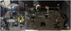 |
Fig. 2 Schematic optical layout of the VIS. The main components are labeled as follows: FPI: Fabry–Perot interferometer; D: detector; L1, L2, L3, L4: achromatic lenses; M1, M2, M4, M5: fixed folding mirrors; M3: removable folding mirror; BS: beam splitter; and PF: prefilter. The red solid line traces the imaging path, while the green dashed line indicates the laser calibration optical path. |
Principal characteristics of the FPI.
Performance specifications of the VIS.
3.2 Data acquisition and model solution
Prior to applying the proposed compensation method, the FPI underwent initial calibration following the manufacturer specifications, with actuator offset voltages set to (Vx, Vy) = (8.64, 7.72) V. The field-dependent wavelength shift at this setting was measured by scanning the Hα spectral line across 37 wavelength points. The scanning was performed by the CS100 controller with a spectral sampling interval of δλ = 0.0455 Å, covering a total range of ±0.819 Å centered at 6562.8 Å. To minimize the influence of solar structural fluctuations, the telescope executed random jitters within a 10′ range during data acquisition. At each wavelength point, 200 frames were captured with a 20 ms exposure time and subsequently averaged to generate flat-field data. After dark-field correction and multi-frame averaging, a three-dimensional data cube was obtained. Using the method described in Sect. 2.1, the displacement of each pixel spectral scanning profile relative to the mean spectrum across the FOV was extracted, giving the field-dependent wavelength shift distribution ∆λ(x′, y′) shown in Fig. 3a. Z-score normalized spectral scanning profiles from four representative positions (top, bottom, left, and right edges) together with the mean spectrum are displayed in Fig. 3b. The cross-correlation values between individual pixel spectrum and the mean spectrum all exceeded 0.98 (Fig. 4), indicating high spectral-matching reliability.
The wavelength shift distribution shown in Fig. 3a exhibits a distinct linear tilt, attributable to nonparallelism between the etalon plates, with a maximum wavelength shift of approximately 0.14 Å. A plane fit was applied to extract the linear drift component, resulting in the distribution displayed in Fig. 5a. This linear drift can be described by the following relation:
 (9)
(9)
The maximum linear wavelength drift across the FOV is ±0.13 Å with slopes (−0.084, 0.124) Å/arcmin. The remaining nonlinear shift component, shown in Fig. 5b, exhibits medium-frequency spatial fluctuations with a maximum amplitude of 0.05 Å. These fluctuations represent the intrinsic bias of the instrument, which cannot be removed by a simple linear correction.
The actuator offset voltages (Vx, Vy)k were set using a CS100 controller, and 30 random voltage combinations were selected across the FPI operational range. For each combination, the corresponding linear drift slope pair (a, b)k was extracted from the measured wavelength shift map. This procedure yielded 30 paired datasets (Vx, Vy)k, (a, b)k for k = 1,…, 30. The optimal control matrix that relates the voltages to the slopes was obtained by solving the resulting least-squares problem with SVD using the full set of 30 datasets. The resulting response model is given by
![Mathematical equation: $\left[ {\matrix{{{V_x}} \hfill \cr {{V_y}} \hfill \cr } } \right] = \left[ {\matrix{{ - 3.052} & {0.012} & {8.386} \cr { - 0.062} & {2.733} & {7.374} \cr } } \right]\left[ {\matrix{a \hfill \cr b \hfill \cr 1 \hfill \cr } } \right].$](/articles/aa/full_html/2026/04/aa58573-25/aa58573-25-eq15.png) (10)
(10)
The accuracy of the response model was validated by generating voltage predictions for each measured slope pair (a, b)k via the Eq. (10). Figure 6 presents a comparison between these predictions and the actual applied voltages. The quantitative assessment yields coefficients of determination of R2 = 0.998 for both Vx and Vy. The corresponding root-mean-square errors (RMSEs) are 0.007 V and 0.006 V, respectively, with a maximum absolute residual of 0.015 V. In the Figs. 6a and b, all data points lie close to the 1:1 line, which is consistent with the high R2 values. The residual distributions of Figs. 6c and d display no systematic trend; the residuals fluctuate randomly around zero and show no correlation with the voltage amplitude. Given the 0.01 V voltage resolution of the FPI CS100 controller, the control accuracy of the model approaches this instrument limit.
For each of the 30 voltage combinations, the corresponding nonlinear wavelength shifts were extracted. Averaging these 30 nonlinear shift maps yielded the mean intrinsic bias distribution of the instrument, as shown in Fig. 7a. The bias exhibits a smooth, intermediate-scale spatial pattern, with a positive shift of approximately +0.05 Å in the central region and negative shifts of about −0.05 Å dominating the lower-left and upper-right areas. The spatial standard deviation (SD) of this mean bias map is 0.014 Å, indicating the amplitude of the bias pattern itself. Fig. 7b presents a different metric: the per-pixel measurement uncertainty. It shows the spatial distribution of the SD computed from the 30 repeated measurements at each pixel. These per-pixel SD values ranges from about 0 Å to 0.011 Å, with a mean of 0.006 Å across the field. To assess the statistical reliability of the mean intrinsic instrument bias, the standard error of the mean (SEM) was evaluated for each pixel using  , where N = 30 and SD is the per-pixel SD shown in Fig. 7b. The pixel-wise SEM values were averaged over the field to obtain a mean SEM of approximately 1.2 × 10⁻³ Å. This value represents the typical precision achieved in determining the mean intrinsic instrument bias after averaging 30 measurements.
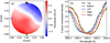 |
Fig. 3 Measurement of the field-dependent wavelength shift. (a) Wavelength shift distribution ∆λ(x′, y′) across the FOV. (b) Z-score normalized spectral scanning profile from four representative edge positions (top, bottom, left, right) compared to the mean spectrum. |
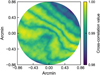 |
Fig. 4 Cross-correlation values between the individual pixel spectrum and the mean spectrum. |
4 Compensation method verification and performance analysis
4.1 Correction results analysis
Based on the plane fit given by Eq. (6), the linear drift component is completely removed when the slopes satisfy a = 0 and b = 0. Substituting this condition into the voltage-to-slope response model of Eq. (10) yields the corresponding offset voltages (Vx0, Vy0) = (8.39, 7.37). Applying these voltages to the FPI actuators actively compensates for linear wavelength drift across the entire FOV.
To validate the correction performance, the field-dependent wavelength shift was re-measured. Compared with the map before compensation in Fig. 3a, the compensated map in Fig. 8a shows a significant reduction of the previously dominant linear component. The maximum wavelength shift decreased from 0.14 Å to 0.05 Å. The spatial distribution closely resembles the mean intrinsic instrument bias shown in Fig. 7a. This distribution has a SD of 0.015 Å, which matches the SD of 0.014 Å for the mean intrinsic bias. A plane fit to the compensated map gives slopes of a = 7 × 10⁻⁴ and b = −5 × 10⁻⁴, both close to zero. These results demonstrate that the linear drift component has been effectively removed, and the residual wavelength shift in Fig. 8a is dominated by the nonlinear intrinsic instrument bias and random noise.
Subtracting the mean intrinsic instrument bias derived in Sect. 3.2 (Fig. 7a) produced the residual map shown in Fig. 8b. This map exhibits a range within ±0.015 Å and a SD of 0.004 Å. The residual shows no linear spatial pattern, which further confirms that the linear drift component has been effectively corrected. However, the residuals display a long-distance spatial correlation, suggesting that the spatial distribution of the nonlinear shift changed. The residual SD of 0.004 Å is comparable to the mean SD of the 30 nonlinear shift measurements (0.006 Å) reported in Sect. 3.2, which demonstrates that the observed change in the nonlinear shift distribution is consistent with the statistical uncertainty previously established for the mean intrinsic instrument bias. Therefore, the long-distance spatial correlation in Fig. 8b may come from two reasons: First, the proposed method primarily corrects for the linear wavelength drift, and there is precision limitation in measuring the nonlinear shift; second, the nonlinear cavity defects of the etalon may not fully coincide before and after compensation.
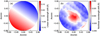 |
Fig. 5 Decomposition of the wavelength shift of the entire FOV. (a) The linear component resulting from the etalon nonparallelism. (b) The remaining nonlinear component representing the intrinsic instrument bias. |
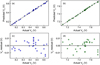 |
Fig. 6 Accuracy validation of the response model. (a) Predicted versus actual voltage for the Vx. The dashed line indicates the 1:1 line. blue spots for Vx, green spots for Vy. (b) Predicted versus actual voltage for the Vy. (c) Distribution of residuals between predicted and actual Vx values. (d) Distribution of residuals between predicted and actual Vy values. |
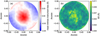 |
Fig. 7 Characterization of the mean intrinsic instrument bias and its statistical uncertainty. (a) Mean intrinsic bias of the instrument. (b) Distribution of the SD computed from the 30 repeated measurements at each pixel. |
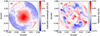 |
Fig. 8 Validation of the linear drift correction. (a) field-dependent wavelength shift distribution after compensation. (b) Residual map after removing the mean intrinsic instrument bias. |
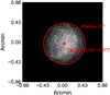 |
Fig. 9 Location and extent of the laser spot. |
4.2 Cross-validation with laser scanning technique
To further assess the reliability of the proposed method, a comparative analysis was carried out against the laser scanning technique (Denker & Tritschler 2005; Reardon & Cavallini 2008). An additional calibration optical path (Fig. 2) was integrated into the VIS setup. A HeNe laser operating at 6329.92 Å was introduced via a movable mirror (M3). The laser beam was collimated by a beam-expanding system consisting of lens groups L4 and L2, entered the etalon perpendicularly, and imaged onto the detector.
As illustrated in Fig. 9, a slight optical-axis misalignment between the calibration and the imaging optical path, together with the finite laser beam diameter of 0.65 mm, resulted in a laser spot centered at (2.42, 1.97)′′ from the center of the FOV. The spot radius was 27′′ , covering 27.7% of the entire FOV. Following the laser scanning technique, the cavity spacing was scanned to obtain laser transmission profiles for each pixel. These profiles were fitted with Gaussian functions. The peak position of each fitted Gaussian profile was then analyzed to derive the two-dimensional distribution of cavity defects and its root-mean-square (RMS) value. The offset voltages Vx and Vy were then varied independently along each direction, and the relationship between the RMS value and the offset voltage was obtained, as shown in Fig. 10, which exhibits a parabolic curve. In each plot, the vertical lines indicate the operating voltages at which the RMS value is minimized, corresponding to (8.337, 7.336) V.
For a direct comparison within the same FOV region, the subarea illuminated by the laser was extracted from the FOV and corrected by the proposed method. The offset voltage-to-linear drift slope response model was re-established specifically for this subarea, resulting in Eq. (11). The optimal voltage derived from this local FOV is (8.338, 7.334) V, differing from the result obtained with the laser scanning technique by only (0.001, −0.002) V. This close agreement further validates the reliability of this proposed compensation method.
![Mathematical equation: $\left[ {\matrix{{{V_x}} \hfill \cr {{V_y}} \hfill \cr } } \right] = \left[ {\matrix{{ - 2.800} & {0.040} & {8.338} \cr { - 0.028} & {2.480} & {7.334} \cr } } \right]\left[ {\matrix{a \hfill \cr b \hfill \cr 1 \hfill \cr } } \right]$](/articles/aa/full_html/2026/04/aa58573-25/aa58573-25-eq17.png) (11)
(11)
The wavelength shift distributions obtained from the two methods at the same offset voltage (8.34, 7.33) V are compared in Fig. 11. Fig. 11a shows the shift measured with the laser scanning technique. The shift map exhibits a fine, speckle-like texture across the field, with positive shifts concentrated near the left-center. The SD of this distribution is 0.018 Å. Fig. 11b presents the shift measured with the method proposed in this study. The image reveals a clear, smooth spatial structure, with positive shifts also concentrated in the left-central portion of the field. The SD of this distribution is 0.012 Å. The SD values derived from the two methods share the same order of magnitude, with the laser scanning technique yielding a slightly higher value. Two main factors contributed to this result. First, the laser scanning technique employed a coherent light source, and the associated laser speckle introduced additional noise. Second, the telecentric illumination in the proposed method resulted in the incident beam covering a small region on the etalon, so that the measurement averaged over the cavity defects within that region.
A discrepancy is observed between this local result and the response model across the entire FOV. This difference can be attributed to the optical-axis misalignment of (2.42, 1.97)′′ and the limited aperture of the laser beam, which does not cover the entire FOV. This discrepancy highlights that the optimal correction depends on the specific FOV used for plane fitting, and that the local sub-FOV and small alignment offsets can both introduce measurable uncertainties.
4.3 Solar observation
To directly evaluate the practical performance of the correction, sunspot group AR14248 was observed using the VIS both before and after field-dependent wavelength drift compensation. Figs. 12a–e present monochromatic images taken before correction at offsets of −0.9 Å, −0.6 Å, 0 Å, +0.6 Å, and +0.9 Å relative to the Hα line core (6562.8 Å). During the spectral scan, a wavelength gradient is evident across the FOV: the lower-left region reaches the Hα line core first in Fig. 12a, followed by a gradual drift of the core position toward the upper-right corner in Figs. 12b–d. By Fig. 12e, the line core appears predominantly in the upper-right region, while the lower-left area has drifted into the continuum. This spatial migration of the line core is a characteristic signature of linear wavelength drift produced by the etalon nonparallelism. After correction, images taken at the same wavelength offset are displayed in Figs. 12f–j. These images show a pronounced suppression of the previously dominant linear drift pattern and an improved homogeneity of the wavelength response across the FOV.
Using the same set of observations described above, the line-of-sight (LOS) velocity fields were derived before and after the linear drift compensation. This compensation corrects the overall wavelength drift caused by etalon nonparallelism. An accurate velocity inversion, however, must also account for nonlinear cavity defects and atmospheric turbulence. Nonlinear cavity defects alter the shape and width of the spectral transmission profile, while atmospheric turbulence distorts the images and couples with those defects. Therefore, a complete velocity field inversion requires a sequence of rigorous data-processing steps to remove the combined influence (Schnerr et al. 2011; de la Cruz Rodríguez et al. 2015). The present study focuses primarily on verifying the effect of linear drift correction, accordingly, an approximate method was adopted to estimate the velocity field. The algorithm uses cross-correlation combined with centroid localization, as detailed in Sect. 2.1, to extract the relative wavelength shift ∆λ(x′, y′) of each pixel spectrum relative to the mean spectrum across the FOV. This shift is then converted into a LOS velocity vr(x′, y′) using the Doppler formula, yielding an approximate velocity field:
 (12)
(12)
where c is the speed of light and λ0 = 6562.8 Å is the central wavelength of the spectral line.
The estimated velocity fields obtained before and after the linear wavelength drift correction are shown in Fig. 13. In the uncorrected case, the velocity field (Fig. 13a) exhibits a large-scale pattern in which the lower-left half of the image is dominated by positive velocities and the upper-right half by negative velocities. This pattern does not correspond to real solar motions but represents an artifact that arises from the linear wavelength drift caused by etalon nonparallelism. The genuine velocity signals of the solar surface are almost entirely buried beneath this strong spurious offset. After applying the linear wavelength drift correction, the velocity field (Fig. 13b) appears completely different. The large-scale artifact is removed, revealing a pattern of fine, mottled small-scale features across the FOV. This structure represents the true velocity signals of the solar surface, free from the dominating instrumental errors.
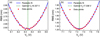 |
Fig. 10 Relationship between the RMS value and the offset voltage. (a) RMS of the cavity defects as a function of offset voltage Vx. (b) RMS of the cavity defects as a function of offset voltage Vy. |
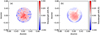 |
Fig. 11 Wavelength shift distributions obtained from the two methods. (a) Wavelength shifts measured by the laser scanning technique. (b) Wavelength shifts measured by the proposed method. |
 |
Fig. 12 Observational validation of the wavelength drift compensation using sunspot group AR14248. (a–e) Monochromatic images before correction at wavelength offsets of −0.9 Å, −0.6 Å, 0 Å (Hα line core), +0.6 Å, and +0.9 Å. (f–j) Corresponding images after correction across the FOV at the same wavelength offsets. |
5 Discussion and conclusions
This study presents and validates a method for compensating linear wavelength drift in telecentric air-gapped FPI instruments. Using solar flat-field data acquired directly within the scientific imaging path, a response model linking actuator offset voltage to the linear drift slope was constructed via SVD. This model achieved R2 = 0.998 for both actuator voltages, with RMSE of 0.007 V and 0.006 V, approaching the instrument limiting voltage resolution of 0.01 V. After correction by this model, the maximum wavelength shift decreased from 0.14 Å to 0.05 Å, and the spatial SD (0.015 Å) matched that of the mean intrinsic instrument bias. A comparison with the laser scanning technique further validated the reliability of the proposed method, with optimal voltages differing by only (0.001, −0.002) V. Application of the method to observations of sunspot group AR14248 in the VIS demonstrated effective suppression of linear drift artifacts, revealing previously obscured solar velocity signals and significantly improving wavelength response homogeneity. These results verify the reliability of the method.
The compensation performance of the proposed method was verified in Sect. 4.3 by comparing the LOS velocities of sunspot group AR 14248 before and after linear drift correction. It should be noted that this comparison employed an approximate method for velocity field derivation. This simplified approach does not account for the influence of nonlinear cavity defects on spectral line shape, width, and symmetry, nor for the coupling between wavefront aberrations induced by atmospheric turbulence and cavity defects. Consequently, the results presented here serve primarily to demonstrate the suppression of linear drift, rather than to provide a precise velocity field. Deriving an accurate velocity map is complex and requires a modified flat-field calibration procedure to effectively correct the impact of nonlinear cavity defects on the measured spectral profiles, as described in previous studies (Schnerr et al. 2011; de la Cruz Rodríguez et al. 2015).
Although the proposed method performs satisfactorily in the VIS, several limitations should be discussed. First, the calibration principle relies on a telecentric configuration, in which the chief rays are parallel to the optical axis. This geometry ensures a one-to-one spatial correspondence between detector pixel and local cavity region, making this technique unsuitable for colli-mated systems. Second, the reliance on quiet-Sun radiation and spectral scan makes the calibration results sensitive to observing conditions. Atmospheric turbulence, seeing variations, and cloud coverage affect image intensity and spectral line stability. Furthermore, the intrinsic solar structure can also influence the results. To mitigate the influence of solar structural fluctuations effectively, a multi-frame averaged flat-field image is required at each wavelength point. In the current implementation, 200 frames were recorded per wavelength point. Combined across 37 wavelength positions and 30 distinct voltage-to-slope datasets, the total correction time reached approximately one hour. However, frequent re-correction is unnecessary for the wavelength drift originating from etalon nonparallelism. Because the parallelism of this type of etalon exhibits good stability and typically remains nearly unchanged over several months (Reardon & Cavallini 2008; Greco et al. 2019). Third, the spatial distribution of the nonlinear shift was observed to differ before and after linear drift compensation. This difference manifests as a long-distance spatial correlation in the residual map (Fig. 8b). Considering the statistical precision of the method for the mean intrinsic instrument bias, this residual pattern may come from the limited precision of the nonlinear shift measurement or from a change in the nonlinear cavity defects during compensation. Although this difference does not affect the linear wavelength drift correction, its origin and the variation in its distribution require systematic investigation in future work.
Despite these limitations, the use of solar flat-field data to compensate linear wavelength drift constitutes a valuable approach. Consequently, the applicability and extension of the proposed method merit further exploration. First, its application to different spectral lines should be investigated, particularly for narrower, velocity-sensitive lines such as Fe I (6173 Å) and He I (10830 Å). A systematic comparison across lines of varying widths and spectral gradients is required to determine the achievable precision and the robustness of the method. Furthermore, significant potential lies in extending the method to more complex FPI configurations, especially multi-etalon systems. Cascade structures improve the spectral purity but also introduce challenges such as cavity spacing coupling and more complicated wavelength tuning (Scharmer 2006). With dedicated study, the present technique could be developed into a more general linear wavelength drift compensation solution applicable to multi-etalon systems.
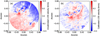 |
Fig. 13 Estimated velocity fields before and after the linear wavelength drift compensation. (a) Estimated velocity fields before correction. (b) Estimated velocity fields after correction. |
Acknowledgements
This work is supported by the National Key R&D Program of China (No. 2024YFA1612000), the Natural Science Foundation of China (Nos. 12573091, 12373115), Yunnan Revitalization Talent Support Program (Nos. 202305AS350029, 202305AT350005), and Yunnan Key Laboratory of Solar Physics and Space Science (No. 202205AG070009). We appreciate all the contributions made by the members of the Astronomical Technology Laboratory and the Fuxian Lake Solar Observatory in operating the Visible-light Imaging Spectrometer (VIS). We also thank Dr. Chris Pietraszewski of IC Optical Systems Ltd. for productive discussions on Fabry–Perot interferometer characterization.
References
- Bailén, F. J., Orozco Suárez, D., & del Toro Iniesta, J. C. 2019, ApJS, 241, 9 [CrossRef] [Google Scholar]
- Bailén, F. J., Orozco Suárez, D., & del Toro Iniesta, J. C. 2021, ApJS, 254, 18 [CrossRef] [Google Scholar]
- Bailén, F. J., Orozco Suárez, D., & del Toro Iniesta, J. C. 2023, Ap& SS, 368, 55 [Google Scholar]
- Beckers, J. M. 1998, A&AS, 129, 191 [Google Scholar]
- Born, M., & Wolf, E. 1999, Principles of Optics: Electromagnetic Theory of Propagation, Interference and Diffraction of Light, 7th edn. (Cambridge: Cambridge University Press) [Google Scholar]
- de la Cruz Rodríguez, J., & van Noort, M. 2017, Space Sci. Rev., 210, 109 [Google Scholar]
- de la Cruz Rodríguez, J., Löfdahl, M. G., Sütterlin, P., Hillberg, T., & Rouppe van der Voort, L. 2015, A&A, 573, A40 [NASA ADS] [CrossRef] [EDP Sciences] [Google Scholar]
- del Toro Iniesta, J. C., Orozco Suárez, D., Álvarez-Herrero, A., et al. 2025, Sol. Phys., 300, 148 [Google Scholar]
- Denker, C., Didkovsky, L., Ma, J., et al. 2003, Astron. Nachr., 324, 332 [Google Scholar]
- Denker, C., & Tritschler, A. 2005, PASP, 117, 1435 [NASA ADS] [CrossRef] [Google Scholar]
- Feng, S., Deng, L., Shu, G., et al. 2012, in 2012 IEEE Fifth International Conference on Advanced Computational Intelligence (ICACI), 626 [Google Scholar]
- Greco, V., Sordini, A., Cauzzi, G., Reardon, K., & Cavallini, F. 2019, A&A, 626, A43 [NASA ADS] [CrossRef] [EDP Sciences] [Google Scholar]
- Halbgewachs, C., Kentischer, T. J., Baumgartner, J., et al. 2024, SPIE Conf. Ser., 13096, 1309617 [Google Scholar]
- Kentischer, T. J., Schmidt, W., von der Lühe, O., et al. 2012, SPIE Conf. Ser., 8446, 844677 [Google Scholar]
- Martínez Pillet, V., del Toro Iniesta, J. C., Álvarez-Herrero, A., et al. 2011, Sol. Phys., 268, 57 [CrossRef] [Google Scholar]
- Puschmann, K. G., Denker, C., Kneer, F., et al. 2012, Astron. Nachr., 333, 880 [NASA ADS] [Google Scholar]
- Puschmann, K. G., Denker, C., Balthasar, H., et al. 2013, Opt. Eng., 52, 081606 [CrossRef] [Google Scholar]
- Reardon, K. P., & Cavallini, F. 2008, A&A, 481, 897 [NASA ADS] [CrossRef] [EDP Sciences] [Google Scholar]
- Righini, A., Cavallini, F., & Reardon, K. P. 2010, A&A, 515, A85 [NASA ADS] [CrossRef] [EDP Sciences] [Google Scholar]
- Ruiz Cobo, B., & del Toro Iniesta, J. C. 1992, ApJ, 398, 375 [Google Scholar]
- Santamarina Guerrero, P., Orozco Suárez, D., Bailén, F. J., & Blanco Rodríguez, J. 2024, A&A, 688, A67 [NASA ADS] [CrossRef] [EDP Sciences] [Google Scholar]
- Scharmer, G. B. 2006, A&A, 447, 1111 [NASA ADS] [CrossRef] [EDP Sciences] [Google Scholar]
- Scharmer, G. B., Narayan, G., Hillberg, T., et al. 2008, ApJ, 689, L69 [Google Scholar]
- Schmidt, W., Bell, A., Halbgewachs, C., et al. 2014, SPIE Conf. Ser., 9147, 91470E [NASA ADS] [Google Scholar]
- Schnerr, R. S., de La Cruz Rodríguez, J., & van Noort, M. 2011, A&A, 534, A45 [NASA ADS] [CrossRef] [EDP Sciences] [Google Scholar]
- Shumko, S., Denker, C. J., Varsik, J., et al. 2002, SPIE Conf. Ser., 4848, 483 [Google Scholar]
- Solanki, S. K., del Toro Iniesta, J. C., Woch, J., et al. 2020, A&A, 642, A11 [NASA ADS] [CrossRef] [EDP Sciences] [Google Scholar]
All Tables
All Figures
|
Fig. 1 Schematic diagram of the telecentric configuration. |
| In the text | |
|
Fig. 2 Schematic optical layout of the VIS. The main components are labeled as follows: FPI: Fabry–Perot interferometer; D: detector; L1, L2, L3, L4: achromatic lenses; M1, M2, M4, M5: fixed folding mirrors; M3: removable folding mirror; BS: beam splitter; and PF: prefilter. The red solid line traces the imaging path, while the green dashed line indicates the laser calibration optical path. |
| In the text | |
|
Fig. 3 Measurement of the field-dependent wavelength shift. (a) Wavelength shift distribution ∆λ(x′, y′) across the FOV. (b) Z-score normalized spectral scanning profile from four representative edge positions (top, bottom, left, right) compared to the mean spectrum. |
| In the text | |
|
Fig. 4 Cross-correlation values between the individual pixel spectrum and the mean spectrum. |
| In the text | |
|
Fig. 5 Decomposition of the wavelength shift of the entire FOV. (a) The linear component resulting from the etalon nonparallelism. (b) The remaining nonlinear component representing the intrinsic instrument bias. |
| In the text | |
|
Fig. 6 Accuracy validation of the response model. (a) Predicted versus actual voltage for the Vx. The dashed line indicates the 1:1 line. blue spots for Vx, green spots for Vy. (b) Predicted versus actual voltage for the Vy. (c) Distribution of residuals between predicted and actual Vx values. (d) Distribution of residuals between predicted and actual Vy values. |
| In the text | |
|
Fig. 7 Characterization of the mean intrinsic instrument bias and its statistical uncertainty. (a) Mean intrinsic bias of the instrument. (b) Distribution of the SD computed from the 30 repeated measurements at each pixel. |
| In the text | |
|
Fig. 8 Validation of the linear drift correction. (a) field-dependent wavelength shift distribution after compensation. (b) Residual map after removing the mean intrinsic instrument bias. |
| In the text | |
|
Fig. 9 Location and extent of the laser spot. |
| In the text | |
|
Fig. 10 Relationship between the RMS value and the offset voltage. (a) RMS of the cavity defects as a function of offset voltage Vx. (b) RMS of the cavity defects as a function of offset voltage Vy. |
| In the text | |
|
Fig. 11 Wavelength shift distributions obtained from the two methods. (a) Wavelength shifts measured by the laser scanning technique. (b) Wavelength shifts measured by the proposed method. |
| In the text | |
|
Fig. 12 Observational validation of the wavelength drift compensation using sunspot group AR14248. (a–e) Monochromatic images before correction at wavelength offsets of −0.9 Å, −0.6 Å, 0 Å (Hα line core), +0.6 Å, and +0.9 Å. (f–j) Corresponding images after correction across the FOV at the same wavelength offsets. |
| In the text | |
|
Fig. 13 Estimated velocity fields before and after the linear wavelength drift compensation. (a) Estimated velocity fields before correction. (b) Estimated velocity fields after correction. |
| In the text | |
Current usage metrics show cumulative count of Article Views (full-text article views including HTML views, PDF and ePub downloads, according to the available data) and Abstracts Views on Vision4Press platform.
Data correspond to usage on the plateform after 2015. The current usage metrics is available 48-96 hours after online publication and is updated daily on week days.
Initial download of the metrics may take a while.