| Issue |
A&A
Volume 708, April 2026
|
|
|---|---|---|
| Article Number | A98 | |
| Number of page(s) | 18 | |
| Section | Stellar structure and evolution | |
| DOI | https://doi.org/10.1051/0004-6361/202558665 | |
| Published online | 01 April 2026 | |
The OWN Survey. A high-resolution spectroscopic survey of southern Galactic O and WN-type stars
I. Project description and single-lined spectroscopic orbits
1
Instituto de Astrofísica de La Plata, CONICET–UNLP, Paseo del Bosque s/n, La Plata, Argentina
2
Facultad de Ciencias Astronómicas y Geofísicas, UNLP. Paseo del Bosque s/n, La Plata, Argentina
3
Las Campanas Observatory, Carnegie Observatories, Casilla 601, La Serena, Chile
4
Departamento de Astronomía, Universidad de La Serena, Av. Juan Cisternas 1200 Norte, La Serena, Chile
5
Centro de Astrobiología. CSIC-INTA, Campus ESAC, C. bajo del castillo s/n, E-28 692 Villanueva de la Cañada, Madrid, Spain
6
Gemini Observatory/NSF’s NOIRLab, Casilla 603, La Serena, Chile
7
Departamento de Astrofísica y Física de la Atmósfera, Universidad Complutense de Madrid, E-28 040 Madrid, Spain
8
Instituto de Astrofísica de Canarias, E-38 200 La Laguna, Tenerife, Spain
9
Departamento de Astrofísica, Universidad de La Laguna, E-38 205 La Laguna, Tenerife, Spain
10
Département d’Astronomie, Université de Genève, Chemin Pegasi 51, CH-1290 Versoix, Switzerland
★★ Corresponding author: This email address is being protected from spambots. You need JavaScript enabled to view it.
Received:
18
December
2025
Accepted:
26
February
2026
Abstract
Context. Massive stars play crucial roles in galactic dynamics and chemical evolution. They are the most significant sources of ionizing UV radiation, their substantial mass-loss rates and explosions inject energy and enrich their surroundings, and their dynamical interactions eject stars and alter the evolution of stellar clusters. Consequently, the study of massive stars is essential for understanding various astrophysical phenomena, including galaxy chemical evolution, interstellar medium dynamics, gamma-ray bursts, and the reionization of the Universe. Key parameters influencing the evolution of massive stars include mass, mass-loss rate, chemical composition, and rotation. The orbits of spectroscopic binaries are particularly valuable because they provide constraints on stellar masses, and when combined with complementary data (e.g., photometry or interferometry), these masses can be fully determined.
Aims. The OWN Survey was started two decades ago to study Galactic O- and WN- (hence the name) type southern spectroscopic binaries. In this paper we present the final results for single-lined (SB1) spectroscopic orbits.
Methods. The OWN Survey carried out a long-term spectroscopic campaign to search for radial velocity variations indicative of orbital motion in a sample of southern Galactic O- and WN-type stars with high-resolution spectrographs in Argentina and Chile. The OWN spectra were later combined with high-resolution spectra from other sources and, in some cases, photometric time series to derive orbits and disentangled spectra, from which masses were constrained or determined and spectral classifications obtained. High-resolution optical spectra of 212 massive stars were obtained during the ∼20 years of the OWN project, and each target was observed at least three times.
Results. Among the 212 stars, 144 exhibited radial-velocity variations greater than 15 km s−1. We present a complete and coherent compilation for the 23 systems with single-lined spectroscopic orbits identified in our sample. In Paper II we will perform a similar analysis for the systems with double-lined spectroscopic orbits.
Key words: binaries: close / binaries: spectroscopic / stars: massive
In Memoriam (1962–2021).
© The Authors 2026
 Open Access article, published by EDP Sciences, under the terms of the Creative Commons Attribution License (https://creativecommons.org/licenses/by/4.0), which permits unrestricted use, distribution, and reproduction in any medium, provided the original work is properly cited.
This article is published in open access under the Subscribe to Open model. This email address is being protected from spambots. You need JavaScript enabled to view it. to support open access publication.
1. Introduction
Massive stars, although few in number, play a crucial role in the dynamic and chemical evolution of their galaxies. In particular, O and Wolf-Rayet (WR) stars are the major sources of ionizing UV radiation, their stellar winds and supernova (SN) explosions have a huge mechanical impact on their surroundings, their nuclear reactions produce many of the chemical elements heavier than hydrogen that are expelled in SN explosions and neutron star mergers, and their dynamical interactions eject stars and significantly alter the dynamics of stellar clusters. Therefore, the study of massive stars is key for many areas of astrophysics, including investigations into the chemical evolution of galaxies, interstellar medium dynamics, origin of gamma-ray bursts and gravitational wave events, and reionization of the early Universe.
The evolution of a massive star is primarily determined by its mass, mass-loss rate, chemical composition, and rotation (e.g. Maeder & Meynet 2000; Meynet & Maeder 2005; Ekström 2021; Li et al. 2023). Massive binaries are particularly important because their binary nature allows for the determination of minimum masses from the radial-velocity (RV) orbital solution. Techniques to infer the orbital inclination can then be used to determine their absolute masses.
Multiplicity introduces uncertainties in the determination of stellar parameters and can significantly affect the evolution of close binaries through Roche-lobe overflow and accretion effects (Hilditch 2001; Sana et al. 2012). It also causes biases in the determination of the initial mass function (IMF) of stellar clusters (Maíz Apellániz 2008). Understanding multiplicity provides clues to the origin of stellar systems; for example, a high frequency of binary systems suggests formation through tidal mergers (Zinnecker & Yorke 2007). In this context, studying massive binaries is essential for advancing our knowledge of stellar evolution and the dynamics of star systems.
It has been established for over two decades that massive stars exhibit higher multiplicities than low-mass main-sequence stars (Preibisch et al. 2001; Sana et al. 2013; Moe & Di Stefano 2017; Guo et al. 2022; Chen et al. 2024). The spectroscopic binary frequency in Galactic clusters rich in O-stars varies enormously among clusters, from 15% to 80%, with no apparent correlation (Mermilliod & García 2001; García & Mermilliod 2001). Additionally, binaries in clusters with fewer O-stars tended to have shorter orbital periods compared to those in clusters richer in O-stars (Zinnecker & Yorke 2007). These findings are based on relatively poor data and incomplete sampling.
Taking into account the above considerations, in 2005 we started the OWN Survey as a long-term project to search for RV variations indicative of orbital motion in a sample of southern Galactic O- and WN-type stars. For the sample we excluded some systems with well-determined spectroscopic orbits at the time, concentrating on those that were poorly or never studied. Our aim was to characterize the multiplicity fraction and to measure stellar masses by applying Kepler’s laws to binary systems, using techniques to derive the orbital inclination when possible.
In the two decades since the launch of the survey, a number of events have conditioned and changed the evolution of the project. The most negative one was the untimely death in 2021 of Rodolfo Barbá, the principal investigator of the project, when this paper and the subsequent one were close to completion. Originally, the sample selection for OWN was based on the Galactic O-Star Catalog (GOSC; Maíz Apellániz 2004) and the VIIth WR catalog (van der Hucht 2001). Later, GOSC led to the Galactic O-Star Spectroscopic Survey (GOSSS, Maíz Apellániz et al. 2011), which uses intermediate-resolution (as opposed to high-resolution) spectroscopy to produce spectral classifications, and in some high-RV amplitude cases, it is able to detect the SB2 nature of some of the OWN systems. GOSC was eventually merged with the Alma Luminous Star (ALS) survey (Pantaleoni González et al. 2021, 2025) to produce the most up-to-date catalog of massive stars. Some of us also launched efforts equivalent to OWN in the northern hemisphere that eventually led to the Multiplicity of Northern O-type Stars survey (MONOS; Maíz Apellániz et al. 2019b; Trigueros Páez et al. 2021; Holgado et al. 2025). In particular, the combination with an equivalent northern-hemisphere survey, IACOB, enabled the quantitative spectroscopic analysis of several samples addressing different specific questions (Holgado et al. 2018, 2020, 2022; Burssens et al. 2020; Britavskiy et al. 2023). Merging the data from OWN, MONOS, IACOB, and other projects together with a search in multiple archives led to LiLiMaRlin, a Library of Libraries of Massive-star high-Resolution spectra (Maíz Apellániz et al. 2019a), a collection of high-resolution spectra of hot (mostly massive) stars that currently has ∼105 epochs. As explained below, all of these projects have contributed in some way or another to the OWN results. For example, Sota et al. (2014) and Maíz Apellániz et al. (2019b) have been pivotal in establishing not only that O stars love company but in that they prefer complex relationships to monogamy, as triple- and higher-order systems are now known to be more frequent than simple binaries.
In addition to the events related to the people involved in the project described in the previous paragraph, others have modified the landscape of massive-star multiplicity in the Milky Way and the Magellanic Clouds. Besides a number of multiplicity surveys, with some that have included stars in the OWN sample as cited below, two space missions have provided highly relevant information. Gaia (Prusti et al. 2016) has produced an immense amount of information on massive stars, including accurate and precise distances. In OWN we use the distances as determined from the third data release (Gaia DR3) for individual stars by Pantaleoni González et al. (2025), and for stellar clusters, we use those determinated by the Villafranca project (Maíz Apellániz et al. 2025). On the other hand, TESS (Ricker et al. 2015) has provided well-sampled light curves that can be used to determine the inclination in eclipsing and ellipsoidal massive binaries, thus completing the missing parameter needed to measure masses in spectroscopic binaries (see Martín-Ravelo et al. 2024; Holgado et al. 2025 for examples).
We have divided the results of the OWN project into two parts: The systems with single-lined spectroscopic orbits (SB1) are published here (Paper I), and the ones with double-lined spectroscopic orbits will appear in Paper II. In addition, we note that some partial results have already appeared at conference proceedings (Gamen et al. 2007, 2008a; Barbá et al. 2010, 2017) or in papers devoted to specific systems (Gamen et al. 2006, 2008b, 2015a,b; Arias et al. 2010; Campillay et al. 2019; Barbá et al. 2020; Putkuri et al. 2021, 2022, 2023; Ansín et al. 2023). Also, some complex systems analyzed with the recently developed software UNWIND, briefly described below, are presented in detail in a separate paper (Maíz Apellániz et al. in prep.). In papers I and II we concentrate on the systems not discussed elsewhere, but we also include a brief summary for the systems in those other papers in order to present the full results of the OWN project.
The SB1 systems are characterized by the detection of radial velocity variations from only one star in the system, while the secondary component remains undetected. The nondetection of the secondary can be due to one of two factors: (a) The secondary star is significantly fainter than the primary, making its spectral lines unobservable in the available data. (b) The companion is a compact stellar remnant, such as a neutron star or black hole. Accurate determination of the orbits in SB1 systems not only provides crucial information about the so-called mass function but also allows for the inference of properties of the secondary component, potentially revealing the existence of compact objects in these massive systems. In this paper, we present the orbital solutions for a significant sample of SB1 systems observed in the OWN Survey, revealing the diversity and complexity of massive binary systems. Given that the next epoch astrometry of Gaia is expected to become available in December 2026 with the fourth data release (DR4) and that it may be able to differentiate between the two options, it is particularly relevant to publish this paper at this time.
In this paper, in Sect. 2 we provide a detailed description of the observations, including the telescopes, instruments, and data collection strategies used in the OWN Survey. We also outline the methods employed for (a) the analysis of RVs, describing the procedures for measuring them from spectroscopic data, identifying orbital periods, and discussing the techniques applied to determine the orbital parameters; (b) the disentangling code UNWIND used to produce the final spectra for each SB1 system; and (c) the techniques used for spectral classification. In Sect. 3, we present the orbital solutions for the SB1 systems, including tables and figures summarizing the derived parameters for each system. Finally, Sect. 4 offers a discussion of the results, focusing on the implications of the detected SB1 orbits.
2. Data and methods
2.1. High-resolution spectroscopy
Within the OWN project we obtained high-resolution optical spectroscopy with instruments at Las Campanas Observatory (LCO), La Silla (ESO), Cerro Tololo Inter-American Observatory (CTIO), and Complejo Astronómico El Leoncito (CASLEO)1. Additionally, for one of our targets, HD 101 190 Aa,Ab, we obtained high-resolution spectra with the recently commissioned Gemini High-resolution Optical Spectrograph (GHOST; Pazder 2020) at Gemini South as part of the System Verification program ID: GS-2023A-SV-104, during selected nights in May 2023.
The OWN observations for this study were carried out over a broad period, from April 2005 to June 2022, excluding the GHOST data. We also included spectra for some Carina targets that were observed at CASLEO for the X-Mega campaign between 1997 and 1999 (Morrell et al. 2001). A summary of the observation runs and data characteristics is provided in Table 1.
Details of the instrumental configurations for OWN observations.
All data, except those from FEROS and GHOST, were reduced using standard echelle routines within the IRAF environment (Tody 1986, 1993). Wavelength calibration was achieved using ThAr lamp exposures taken in proximity to the stellar observations at the same telescope position. The reduction of FEROS spectra was carried out using the ESO-MIDAS pipeline, which provides data analysis tools maintained by ESO. The GHOST spectra were processed using the GHOSTDR software, version 1.0.0, operating within the DRAGONS 3.0 framework (Ireland et al. 2018; Hayes et al. 2022; Labrie et al. 2019, 2022).
Additionally, we used LiLiMaRlin spectroscopy (Maíz Apellániz et al. 2019a) from six spectrographs: HARPS-N at TNG, FIES at NOT, and HERMES at Mercator, the Observatorio del Roque de los Muchachos (La Palma, Spain); UVES at VLT, Observatorio Paranal (Chile); and HARPS at 3.6 m and FEROS at 2.2 m, Observatorio de La Silla (Chile). With the LiLiMaRlin data we independently verified the orbits and applied the disentangling code UNWIND (see Sect. 2.4) to obtain rectified, high-S/N, interstellar medium (ISM)-subtracted, and velocity-corrected spectra for spectral classification.
2.2. TESS photometry
We used public TESS photometric data to search for variability in some specific targets. The light curves were generated using the Lightkurve Python package, designed for analyzing Kepler and TESS data (Lightkurve Collaboration 2018).
2.3. RV analysis
We fit the spectral lines using Gaussian functions via the SPLOT task in IRAF. In most cases, we measured RVs from the He IIλ4542, λ4686, λ5412, and He Iλ5876 absorption lines. We also measured the Na Iλλ5890–96 interstellar (IS) lines for comparison. The RVs from lines with similar behavior (mean, standard deviation, and RV difference) were averaged, typically from the He II absorption lines, although He IIλ4686 was excluded for giants and supergiants due to contamination by emission. The IS lines showed no significant systematic differences across the spectrographs.
Given an expected internal RV uncertainty of ∼3 km s−1, we adopted conservative thresholds to minimize false detections. Variations below 15 km s−1 (∼5σ) were considered consistent with constant RVs. A higher threshold of 19 km s−1 (> 6σ) was adopted to securely identify RV-variable stars (RVvar), leaving the 15–19 km s−1 range as a transition region populated by RV-variable candidates (Fig. 1). RVvar stars were analyzed for periodicities using the Lomb-Scargle method, provided by the NASA Exoplanet Archive. Once a probable period was found, orbital parameters were calculated using the GBART program (Bareilles 2017). If GBART failed, the FOTEL program (Hadrava 2004), more suited for eccentric orbits and differential systemic velocities, was used.
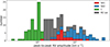 |
Fig. 1. Stacked histogram of the peak-to-peak RV amplitudes for the 212 targets of the OWN sample, showing the relative contributions of SB1, SB2, RV variables, and constant RV (C) systems. The horizontal scale is logarithmic. |
We present systems with determined SB1 orbits but no SB2 solution, including both intrinsically single-lined binaries and cases where the secondary contribution is undetectable or too complex. Individual objects are discussed in Sect. 3.
2.4. The disentangling code UNWIND
We have recently developed a new spectral disentangling code called UNWIND that will be discussed in detail in an upcoming paper (Maíz Apellániz et al. in prep.). That paper will include the detailed analysis of one SB1 orbit briefly presented here (HD 101 190 Aa,Ab) and other SB2 orbits briefly discussed in Paper II among other examples. The main UNWIND code includes modules for (a) rectification, (b) ISM subtraction (including a new ISM model covering the optical and NIR), and (c) the disentangling itself. It includes a spectral library to be used as seeds and tools for cross-correlating and profile-fitting the data from the disentangled spectra and for orbit determination.
The SB1 systems do not require spectral disentangling (unless a weak companion is being searched for). However, they still benefit from UNWIND, which produces what we refer to as “joined” spectra: rectified, ISM-subtracted, velocity-shifted, and median-combined spectra that provide a clean, high-S/N output suitable for spectral classification (see Sect. 2.5). In Paper II, UNWIND will be used to produce disentangled spectra for systems identified as SB2.
Spectrograms are shown on Fig. A.1, degraded to the spectral classification resolution of R = 2500. The first three panels correspond to UNWIND joined spectra (marked by a J in Table A.2). The last panel corresponds to spectra where we could not obtain a clean result with UNWIND, and are marked by a G or L in Table A.2, corresponding to their origin in GOSSS (Maíz Apellániz et al. 2011) or LiLiMaRlin data, respectively.
2.5. Spectral classification
The spectrograms in Fig. A.1 were classified using Marxist Ghost Buster (MGB, Maíz Apellániz et al. 2012) and a new grid of spectral classification for OB stars (Maíz Apellániz et al. in prep.) that updates the one used in Maíz Apellániz et al. (2016). MGB is a code that applies the principles of spectral classification (Maíz Apellániz et al. 2026) by visually comparing the observed spectrum with a spectral classification grid at the same spectral resolution. As spectral classification is usually done at R = 2500, this requires degrading the resolution of the LiLiMaRlin data, which has the benefit of providing a very high S/N (indeed, significantly higher than what is traditional in the field). The combination of the same resolution and the high S/N allows for an accurate determination of the n index (Fig. 4 in Maíz Apellániz et al. 2026). The spectral types are listed in Table A.2, along with the spectroscopic binarity status (SBS) nomenclature of Maíz Apellániz et al. (2019b) for each system.
3. SB1 orbits
From the RV analysis of the entire sample comprised by 212 stars (see Fig. 1), the OWN Survey identified only 67 targets with variations below the conservative threshold of 15 km s−1; in other words, 68% of the sample is RV-variable or a multiple-system candidate. Among the remaining objects, 74 of them did not show any reliable periodicity and therefore require continued spectroscopic monitoring. For 71 targets, orbital parameters could be determined. Among them, we present 24 SB1 orbits corresponding to 23 stars, as one object hosts two independent SB1 systems (SB1+SB1). The corresponding RV curves are shown in Figs. 2 and 3.
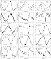 |
Fig. 2. Radial velocity curves for OWN targets identified as SB1. Filled circles represent the RVs determined for the primary components. |
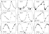 |
Fig. 3. Radial velocity curves for OWN targets identified as SB1. Filled circles represent the RVs determined for the primary components. |
3.1. τ CMa Aa,Ab (= 30 CMa Aa,Ab = HD 57 061 Aa,Ab = GLS 14 805 Aa,Ab)
The star τ CMa has been known to have an O-type SB1 system with a period close to 155 d for almost a century (Struve & Pogo 1928) but results in the last decades have revealed it to be a complex system with four OB stars and two additional orbits besides the spectroscopic one, an eclipsing (more properly, ellipsoidal) one and a visual one (van Leeuwen & van Genderen 1997; Maíz Apellániz & Barbá 2020). Maíz Apellániz & Barbá (2020) used spatially resolved spectroscopy to identify that both visual components (Aa and Ab) are O stars.
Given the complexity of the system, in addition to the OWN spectroscopy we conducted several specific LiLiMaRlin campaigns with FEROS, FIES, and HERMES during 2025 to analyze τ CMa in more detail. For the results, presented in more detail in an incoming paper (Maíz Apellániz et al. in prep., see also Rosu et al. 2025), we used UNWIND to disentangle the different components. They indicate that (a) Ab is an O9.2 II single star in a ∼350 a orbit around Aa, which itself is composed of (b) an OC8.5 Ib((f)) primary that traces the spectroscopic SB1 orbit around a (c) pair of fast-rotating early-B stars whose mutual orbit is the cause of the 1.282 d photometric period. The system is included here because at this point we have been only able to calculate the Aa1 SB1 orbit given the difficulty in detecting the two fainter, fast-rotating B stars in Aa2. We also note that the spectral classifications changed slightly due to a re-estimation of the contribution from the B+B binary, hence the differences between the results here and in Maíz Apellániz & Barbá (2020).
3.2. NX Vel A,B (= HD 73 882 A,B = GLS 1110 A,B)
The NX Vel system is known to include at least one eclipsing binary and is located behind the Vela supernova remnant and within the Gum Nebula. The photometric period has been a subject of some uncertainty. The HIPPARCOS and TYCHO catalogs (Perryman et al. 1997) reported a period of P = 1.46 d, but Otero (2003), using combined Hipparcos and ASAS-3 data, found a period of 2.9199 d, suggesting that the eclipses differ in depth. More recently, Mellon et al. (2019) refined the period to P = 2.91834 ± 0.0003 d. However, despite these photometric observations, no definitive RV orbit had been identified. Feast et al. (1955) classified the star as RV-variable but did not determine any orbit. The system is a visual binary with the B component having a Δm of 1.3 mag and a separation of 668 mas (Aldoretta et al. 2015) with respect to A.
Our analysis revealed that the He II absorption lines do not correlate with the photometric period. Instead, they trace an orbit with a period of P ∼ 13.06 d (see Fig. 2). Interestingly, the RV variations of He I differ from those of He II, but when plotted against the shorter period of P ∼ 2.9 d, the He I RVs suggest a potential orbital solution (see Fig. 2). This suggests the existence of two binaries, one in A and another in B. The two RV curves show a significant scatter, a sign of cross-contamination, indicating that the short-period binary likely contains an early-B star. We attempted a disentangling of the system with UNWIND but the combination of low-velocity amplitudes and small number of LiLiMaRlin epochs did not allow us to obtain a successful result. Therefore, the spectrogram shown in Fig. A.1 is from a single LiLiMaRlin epoch and we are unable to produce separate spectral types (Table A.2). The spectral type of O8.5 IV(n) is the same as in Sota et al. (2014) but with an added (n) suffix, because lines are broadened.
We constructed the system’s light curve using TESS data from sectors 8, 35, 61, and 62. A period of P = 2.9199 ± 0.0015 d was derived using the MARMUZ code (Marraco & Muzzio 1980), which is consistent with previous findings. A preliminary light curve is shown in Fig. 4 (top panel), where two eclipsing-like features can be observed. Surprisingly, their periodicity matches that of the He II lines, indicating that the O-type star is also part of an eclipsing system.
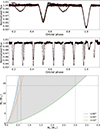 |
Fig. 4. First panel: Light curve of NX Vel A,B, using the period P = 2.9199 d (only TESS sector 61). Second panel: Same but with the period P = 13.0734 d, obtained from the He II absorption lines. Third panel: Mass-function plot for the NX Vel A spectroscopic orbit. |
To estimate the expected mass of the secondary component in A, we calculated its value across a range of orbital inclinations, assuming a fixed absolute mass for the primary (from Martins et al. 2005) and using the obtained mass function. The expected mass of the secondary component in the A-pair was found to be in the range of 0.5–3 M⊙ (Fig. 4, third panel). Given its eclipsing nature, it is most likely close to 0.5 M⊙, and approximately 11 mag fainter than the primary, which explains why it remains undetected in the composite spectrum.
In conclusion, our data confirm that NX Vel A is an eclipsing SB1 system with a P = 13.0630 d period and an O-type primary. Additionally, the fainter B companion is itself a double-eclipsing SB1 system with a P = 2.9199 d period and likely containing an early-B star. Further analysis is required and will be presented in a future publication.
3.3. HD 75 211 (= GLS 1154)
Prior to OWN, this star had only one previously published RV measurement (Conti et al. 1977). It was classified as an SB1 by Chini et al. (2012), though no orbital solution was provided. We present a determination of its RV orbit in Table A.1. In our solution, we incorporated a FEROS spectrum obtained from the ESO database. We averaged the RVs of the He IIλ4542 and λ5412, He Iλ5015, and O IIIλ5592 lines, as they showed consistent behavior in terms of their mean, standard deviation, and maximum variation across nearly 100 spectra.
The UNWIND-joined spectrum of HD 75 211, produced from six LiLiMaRlin epochs, yields a spectral classification of O8.5 II((f)), the same as in Sota et al. (2014). Given its luminosity class, we conducted intensive monitoring at CASLEO to investigate potential pulsations. For instance, on January 26, 2022, we observed the star for 6.6 hours (the orbital period is P = 20.44 d), detecting a variation of nearly 8 km s−1. A similar result was obtained during observations on January 13, 2023. Therefore, the scatter observed in Fig. 2 is likely intrinsic, and most probably linked to pulsations. The pulsational analysis will be published in a future paper.
Prior to the publication of this paper, Mahy et al. (2022) published an SB1 orbit of HD 75 211 with similar parameters except for a large eccentricity of 0.340 ± 0.009 (our orbit is close to but not circular). Given the pulsational character of the star and the small number of epochs in their solution (their Fig. 1), our solution is likely more reliable.
3.4. LM Vel (= HD 74 194 = GLS 1116)
The orbital solution of the optical counterpart of the prototype of the Super Fast X-Ray Transients (SFXT) was published in Gamen et al. (2015a). After that publication, we secured new spectra. Thus, the new orbital parameters in Table A.1 are obtained with the increased RV dataset. The UNWIND-joined spectrum of LM Vel, produced from 21 LiLiMaRlin epochs, yields a spectral classification of O8.5 II(n)((f))p, making this an Onfp star (Maíz Apellániz et al. 2026, see also Sota et al. 2014).
Mahy et al. (2022) published an alternative orbit with similar parameters, with the exception of ω. Similarly to HD 75 211, their orbit is based on fewer epochs (22) than ours, and the significant scatter in Fig. 2 points towards the existence of pulsations in this luminosity class II object, leaning towards the higher reliability of our result.
We assign the value of the spectroscopic mass 23.4 ± 5.0 M⊙ from Holgado et al. (2025) to the visible component of LM Vel. Using that value and the mass function of the system, the inferred mass of the compact companion ranges from 1.3 to 9.4 M⊙ for inclinations of 90° and 10°, respectively. Therefore, neutron-star masses (up to ∼2.4 M⊙) are still possible, even for relatively low inclinations, down to about 35°.
3.5. CPD −47 2963 A,B (= GLS 1216 A,B)
The star CPD −47 2963 has an entry in the General Catalogue of Stellar Radial Velocities (Wilson 1953), but its RV is of poor quality. Our initial observations led us to classify it as an SB1 with a period of approximately 58 days (Sota et al. 2014), but further data ruled out this periodicity. Le Bouquin et al. (2017) determined the astrometric orbit of this target, finding P = 656 ± 2.9 d and e = 0.662 ± 0.013.
We derived a moderately scattered SB1 orbit using the averaged RVs of four absorption lines: He IIλ4542 and λ5412, He Iλ5876, and O IIIλ5592. Periodicity analysis of the RVs was conducted using the MARMUZ program (Marraco & Muzzio 1980), which identified five probable periods: 654 d, 327 d, 163.5 d, 490.7 d, and 235 d. Except for 235 d, these are aliases (0.5, 0.25, and 0.75) of the most probable period, 654 d.
We confirmed the periodicity by analyzing the epochs of extreme RVs, occurring in March 2021, January 2023, and November 2024, separated by approximately 650 days. Subsequently, we used FOTEL, allowing all parameters to vary freely, and obtained a period of P = 652.5 d (Table A.1), which is consistent with the astrometric solution, including the eccentricity.
The UNWIND-joined spectrum of CPD −47 2963 A,B, produced from six LiLiMaRlin epochs, yields a spectral classification of O5 Ifc, the same as in Sota et al. (2014). Given its supergiant nature, we monitored this star intensively over several nights, finding an intrinsic RV variability of about 6 km s−1. This suggests the orbit is reliable despite the observed scatter.
We attempted to detect the companion in the LiLiMaRlin spectra to determine an SB2 orbit, something that should be possible in principle given the Δm of 1.4 mag (Sana et al. 2014). However, the expected small velocity separation and the small number of epochs did not allow us to do so. We plan on obtaining more epochs to reach this goal.
3.6. HD 76 968 (= GLS 1214)
The star HD 76 968 was first classified as RV variable by Feast et al. (1955) based on just six measurements. Photometric variability was also noted by Gaposchkin (1955) and more recently confirmed by Lefèvre et al. (2009), who reported a periodicity of 5.751 d. Chini et al. (2012) listed two entries for this star: one as an O9.7 Ib and SB1, and the other as a B0 II and SB2.
We derived the orbital solution using our own spectra, averaging the RVs of He IIλ4542, He Iλ5876, and O IIIλ5592 lines. Similar to HD 75 211, we monitored this star from CASLEO to investigate the potential influence of pulsations on its RVs. A continuous series of spectra collected over nearly five hours revealed an intrinsic scatter of approximately 7 km s−1 (not related with the orbital period which is 26.957 d). The detailed pulsational analysis will be presented in a future publication. The UNWIND-joined spectrum of HD 76 968, produced from eight LiLiMaRlin epochs, yields a spectral classification of O9.2 Ib, the same as in Sota et al. (2014).
3.7. HD 91 572 (= GLS 1640)
There is no prior analysis of the RVs for this early-type star, except for the SB1 classification reported by Chini et al. (2012). Using FOTEL, we derived a reliable orbital solution based on the averaged RVs of the He II lines, yielding a period of approximately four years. The most recent RV minimum, which closely coincided with the periastron passage, occurred in March 2023, and the next one is anticipated around April 2027. The UNWIND-joined spectrum of HD 91 572, produced from six LiLiMaRlin epochs, yields a spectral classification of O7 V((f)), slightly later than the O6.5 V((f))z one in Sota et al. (2014).
3.8. HD 94 024 (= GLS 1952)
Prior to OWN, HD 94 024 had no published RV in the bibliography. Chini et al. (2012) identified this star as SB1 and Maíz Apellániz et al. (2018b) identified it as a runaway star likely expelled from the Car OB1 association. More recently, Mahy et al. (2022) derived an SB1 orbit forcing the eccentricity to be zero. We also derived an SB1 orbit leaving e as a free parameter, but the result indicates that it is extremely low anyway (two sigmas away from zero), and thus it is compatible with the previous determined orbit. The UNWIND-joined spectrum of HD 94 024, produced from eight LiLiMaRlin epochs, yields a spectral classification of O8 IV, the same as in Sota et al. (2014).
3.9. CPD −59 2600 (= GLS 1856)
The RVs of CPD –59 2600 were analyzed by Levato et al. (1991, ten consecutive nights), who found them to be constant. Later, Chini et al. (2012) classified this star as an SB2 system.
We derived a new orbital solution using the average RVs of the He II absorption lines from the primary component. Additionally, we identified very broadened He Iλ5876 and λ4471 absorption lines, which appear to belong to the secondary component based on their positions in different orbital phases. However, during the expected quadrature phase, where the secondary should shift towards the blue, its spectral features are only marginally detected, preventing a reliable determination of its orbital motion. Thus, we present only the SB1 orbit here (depicted in Fig. 2). We also attempted the detection of the secondary using UNWIND and nine available LiLiMaRlin epochs assuming different values of the mass ratio. However, we were unsuccessful, likely because of the combination of small velocity separation and small number of epochs. Given the line-profile changes in the He I lines, we used the LiLiMaRlin epoch with the largest velocity separation to obtain a spectral classification of O5.5 V((f)) + OB. In Sota et al. (2014) the single-component classification was O6 V((f)), with the primary slightly contaminated by the secondary (Fig. A.1).
3.10. HD 96 946 (= GLS 2185)
There are only two RV measurements available in the Simbad database, but no epochs are provided (Evans 1967; Martin 1964). Chini et al. (2012) identified this star as an SB1 system.
Our spectroscopic data reveal clear RV variations with a well-defined periodicity. We computed the SB1 orbital solution, which is presented in Fig. 2. Further analysis is required to fully characterize the nature of the secondary companion and to investigate the scatter in the RV curve, particularly around the periastron passage (orbital phase ϕ = 0.0). The UNWIND-joined spectrum of HD 96 946, produced from seven LiLiMaRlin epochs, yields a spectral classification of O6.5 III(f), the same as in Sota et al. (2014).
3.11. HD 101 190 Aa,Ab (= GLS 2424 Aa,Ab)
The HD 101 190 Aa,Ab system is a visual binary with a ΔH of 0.62 mag and a separation of 25.73 mas (Sana et al. 2014) and is located in IC 2944 at a distance of  kpc (Pantaleoni González et al. 2025), leading to a distance in the plane of the sky around 64 au. Therefore, we expect a small velocity difference between the two visual components and with little change in 20 years. The integrated spectra from the two visual components shows a short-period (6.04654 ± 0.00018 d) SB1 orbit, indicating that HD 101 190 Aa,Ab is composed of a constant-velocity star and an SB1 system. Given its complexity, we analyzed HD 101 190 Aa,Ab in a separate paper (Maíz Apellániz et al. in prep.), where we used UNWIND to disentangle the spectra and determine that Aa is the one with constant velocity and a very early O star [classified as O3.5 IV((f))] and Ab is the SB1 system with a later O classification of O8 III((f)).
3.12. HD 101 205 A,B (= V871 Cen A,B = GLS 2427 A,B)
The system HD 101 205 A,B, another member of IC 2944, was first identified as an RV variable by Thackeray & Wesselink (1965) and Conti et al. (1977), and later classified as an SB2 system by Chini et al. (2012), although no orbital solution was provided. McAlister et al. (1990) discovered a speckle companion at a separation of 0.362 mas.
Photometrically, Mayer et al. (1992) reported the star as an eclipsing variable, noting that Balona (1992) also identified it as such, though with an erroneous designation of HD 101 191. Both studies determined a period of approximately 2.08 d. Other subsequent works confirmed these findings until Zasche et al. (2022) identified it as a candidate for a multiple eclipsing system based on TESS data. They detected two periodicities: 2.8170 d and the previously known 2.09 d.
Given the absence of a spectroscopic orbit at the time of this study, we observed HD 101 205 A,B and determined an SB1 orbit with a period of P = 2.82030 ± 0.00003 d. The RV curve shows significant scatter, prompting an analysis of the residuals, which revealed a likely period of 1.0433 d, approximately half of the photometric 2.09 d period.
Further investigation is required to fully understand this intriguing system but the most likely explanation lies in the fact that it is a visual binary with a separation of 0 4 and a Δm of 0.3 mag (Mason et al. 2001) and that some LiLiMaRlin epochs show double lines even at a resolution of 2500 (Fig. A.1). We tried disentangling the system with UNWIND but we were unsuccessful, as it looks as though there are at least three lights contributing to the spectra. Zasche et al. (2022) favored a configuration with the two eclipsing pairs being Aa1,Aa2 and Ab2,Ab2, bringing the total number of objects to 5 when including B. However, we find that unlikely, as B in that configuration would be static but still contribute a significant fraction of the light, while the evidence in the disentangling attempts suggest that the two brightest contributors to the spectra move. Therefore, we suggest as more likely a configuration with Aa,Ab and Ba,Bb being the two eclipsing pairs, which is simpler as it contains only four stars instead of five. As we are only able to provide an SB1 orbit, we leave the SBS as SB1E+Ea, but that should change in the future with better data, leading to SB1E+SB1Ea or SB2E+SB1Ea.
As we could not disentangle the system, we used a LiLiMaRlin epoch with double lines (Fig. A.1) to derive a spectral classification of O6 III(n)(f) + B0: V:, which differs from the single-component classification of O7 II:(n) of Sota et al. (2014) and is likely to change in the future. Given the configuration of the system, the star dominating the O6 spectrum is likely to be Aa and the one dominating the B0 spectrum is likely to be Ab. This target would be an excellent target for spatially resolved spectroscopy using either STIS (Maíz Apellániz & Barbá 2020) or lucky spectroscopy Maíz Apellániz et al. (2018a, 2021).
3.13. HD 112 244 (= GLS 14 976)
The orbital solution for this target, along with its key background information, is described in Mayer et al. (2017). Using our set of 41 spectra, we obtained a similar orbital solution. We applied FOTEL to the mean RVs of He IIλλ4542 and 5412. The resulting scattered RV curve closely resembles the one presented by Mayer et al. (2017). The UNWIND-joined spectrum of HD 112 244, produced from 31 LiLiMaRlin epochs, yields a spectral classification of O8.5 Ib(f)p, similar to that of Sota et al. (2014) but changing the luminosity class from Iab to Ib due to the improvement in S/N.
3.14. HD 124 314 Aa,Ab (= GLS 3212 Aa,Ab)
It has long been recognized as an RV-variable star in the literature (see e.g., Feast et al. 1955; Buscombe & Kennedy 1969; Conti et al. 1977; Chini et al. 2012), but no orbital solution has been published. We identified a likely periodicity in the averaged RVs of the He IIλ4686 and λ5412 lines. However, the data exhibit significant scatter, exceeding the expected uncertainties, and additional spectra are needed to confirm this result.
Sana et al. (2014) identified a visual companion with a separation over 1 mas but with two somewhat discrepant measurements. As they mentioned, the spectroscopic binary detected by us in OWN is likely their visual binary but note that their two ΔH measurements of 2.21 ± 1.75 mag and 0.66 ± 0.44 mag leave enough room for the companion to be easily detected in the spectra or not. The lack of noticeable profile changes in the observed lines makes us lean towards a magnitude difference larger than 1 mag. The UNWIND-joined spectrum of HD 124 314 Aa,Ab, produced from 28 LiLiMaRlin epochs, yields a spectral classification of O6 IV(n)((f)), the same one as in Sota et al. (2014). The system also includes a more distant pair Ba,Bb, which is far enough (∼3″) not to be included in the spectra analyzed here, and also includes an O star, classified by Sota et al. (2014) as O9.2 IV(n).
3.15. HD 130 298 (= GLS 3284)
The star HD 130 298 was first noted as a probable RV variable by Feast et al. (1963). Later, Hubrig et al. (2011) reported evidence of a magnetic field in this star, and Chini et al. (2012) classified it as an SB2 system. SB1 orbital solutions were subsequently determined by Mayer et al. (2014) and Mahy et al. (2022).
In this study, we measured and averaged a larger set of spectral lines than usual, He IIλ4200, λ4542, λ5412, and He Iλ4471, λ5016, λ5876, in an attempt to detect the secondary component identified by Chini et al. (2012). However, our efforts were unsuccessful, consistent with the findings of Mayer et al. (2014). We inspected spectra with extreme RV values and found slight asymmetry in the profiles, but this asymmetry was consistent across both quadratures. We present here the SB1 orbital elements, based on the mean RVs of the six lines, which are in agreement with the previously published orbits. The UNWIND-joined spectrum of HD 130 298, produced from ten LiLiMaRlin epochs, yields a spectral classification of O6.5 III(f), similar to the one in Sota et al. (2014) but without the (n) suffix.
3.16. HD 152 424 (= GLS 3829)
Radial velocity variations for HD 152 424 have been reported in several studies: Struve (1944) listed it as a ‘spectroscopic binary?’, Hill et al. (1974) suggested it might be a long-period system, and Garmany et al. (1980), based on two measurements, noted it as ‘variable?’. Levato et al. (1988) also detected RV changes but attributed them to causes other than orbital motion. Later, Chini et al. (2012) classified it as an SB1, and Sota et al. (2014), using preliminary OWN data, confirmed a similar identification.
We present the first orbital solution for HD 152 424, based on high-resolution data collected over 22 years, including a 2025 LiLiMaRlin campaign. The system exhibits a long period, P = 216.79 ± 0.08 d, and a high eccentricity, e = 0.72 ± 0.02. However, the derived eccentricity strongly depends on the few measurements obtained near the RV extrema. More epochs near those phases are needed to improve the orbit. We used 33 LiLiMaRlin epochs to obtain an UNWIND-joined spectrum of the star and derive a spectral classification of OC9.2 Ia. This is the same classification as in Sota et al. (2014).
3.17. HD 152 405 (= GLS 3827)
Sanford (1949) reported a single RV measurement for this star, although the observation date was not specified. Later, Feast et al. (1955) provided six additional RV measurements and suggested that HD 152 405 might be a potential SB2. Conti et al. (1977) contributed one more value, while Raboud (1996) confirmed its RV variability with four further measurements. The star was classified as SB1 by Chini et al. (2012), and more recently as SB2 by Mahy et al. (2022), though no RVs for the secondary component were given. They uncovered the secondary’s spectral features through a disentangling method, classifying it as a B1 star and determining a semi-amplitude of K2 = 79.38 km s−1.
We collected 113 spectra of HD 152 405, which clearly showed RV variability. The orbital solution was derived by averaging the RVs of He Iλ4009, λ5016, and λ5876, along with He IIλ4200 and λ4686 absorption lines, following the same approach used for other supergiants. The orbital parameters we obtained are consistent with those reported by Mahy et al. (2022), although we did not detect any spectral features associated with the secondary component. The effects of pulsations, which seem to distort the line profiles and influence the RV measurements, will be addressed in a future study. We used 10 LiLiMaRlin epochs to obtain an UNWIND-joined spectrum of the star and derive a spectral classification of O9.7 II. This is the same classification as in Sota et al. (2014).
3.18. HD 152 723 Aa,Ab (= GLS 3854 Aa,Ab)
The HD 152 723 Aa,Ab system is a visual binary with a ΔH of 1.7–2.0 mag (Sana et al. 2014). Feast et al. (1955) provided five RV measurements for this star, while Conti et al. (1977) added one more. Fullerton et al. (1996) reported RV variability in HD 152 723 Aa,Ab, although no specific RV values were published. Both Chini et al. (2012) and Mahy et al. (2022) classified the star as SB2. The latter study revealed secondary spectral features, such as Si II, using a disentangling technique, classifying the secondary as a B5 star and determining a semi-amplitude of K2 = 89.37 km s−1.
We obtained 95 spectra of HD 152 723 Aa,Ab. Using the averaged RVs of He IIλ4542, λ4686, and λ5412, He Iλ5876, and O IIIλ5592 absorption lines, we obtained a scattered and highly eccentric orbit SB1 with a relatively short period (P = 18.8964 ± 0.0009 d), consistent with the one Mahy et al. (2022).
Given the presence of a companion expected to contribute ∼15% of the flux in the B band, we analyzed HD 152 723 Aa,Ab in a manner analogous to what we did for HD 101 190 Aa,Ab. We assumed the presence of two lights, one (Aa) contributing 85% of the flux following the SB1 orbit and another one (Ab) with 15% of the light and constant velocity. The results are presented in detail in a separate paper (Maíz Apellániz et al. in prep.), where we used UNWIND to disentangle the spectra and determine that Aa has an O6 III(f) spectrum and Ab is a B2 Vn. The residuals of the process are much lower than the ones we obtain if the SB2 orbit of Mahy et al. (2022) is used instead.
3.19. HDE 322 417 (= GLS 3873)
No previously published RVs for HDE 322 417 were found in the consulted bibliography, with the only reference being Chini et al. (2012), who did not detect any RV variations. We gathered 24 spectra, which show RV variations of up to 40 km s−1. These variations are consistent with orbital motion, and we derived the corresponding parameters using the average RVs of the He IIλ4542 and λ5412 lines. The UNWIND-joined spectrum of HDE 322 417, produced from six LiLiMaRlin epochs, yields a spectral classification of O6.5 IV((f)), the same as that of Sota et al. (2014).
3.20. HD 154 643 (= GLS 3941)
This star has limited RV measurements in the literature (Buscombe & Kennedy 1969; Thackeray et al. 1973). The latter suggested RV variability based on discrepancies between both studies. Chini et al. (2012) classified this star as SB1, while more recently Burssens et al. (2020) reported stochastic low-frequency variability combined with rotational modulation in TESS data.
Our set of 32 spectra reveals RV variations consistent with the range of previously published values. We derived the orbital parameters, which suggest a highly eccentric orbit (e = 0.641 ± 0.007) with a period of approximately one month. The UNWIND-joined spectrum of HD 154 643, produced from five LiLiMaRlin epochs, yields a spectral classification of O9.7 III, the same as that of Sota et al. (2014).
3.21. HDE 319 699 (= GLS 4078)
The star HDE 319 699 is one of the earliest members of the young open cluster NGC 6334. The only study addressing its multiplicity is by Chini et al. (2012), who classified the star as an SB1, though no orbital solution was provided. Here we derive its first ever spectroscopic orbit.
The spectral profiles show variability and asymmetry, yet no evidence of a secondary companion has been detected so far. We are continuing our efforts to identify the secondary, a task that will be explored in detail in a future study. The UNWIND-joined spectrum of HD 154 643, produced from five LiLiMaRlin epochs, yields a spectral classification of O5 V((fc)), the same as that of Sota et al. (2014).
3.22. HD 163 892 (= GLS 4523)
This star was reported as variable by Conti et al. (1977), likely because they obtained a different RV compared to earlier measurements by Neubauer (1943; −14.5 km s−1) and Feast et al. (1963; −15, 13, and 18 km s−1). Chini et al. (2012) identified the star as an SB1, and Mayer et al. (2014) derived both the period and orbital solution for this system.
We obtained a similar orbital solution to that of Mayer et al. (2014), though their solution is somewhat incomplete due to a lack of RV measurements near the maximum (see their figure 7). Our more robust solution, shown in Table A.1, incorporates RV data from Feast & Thackeray (1963), Conti et al. (1977), as well as two measurements from Mayer et al. (2014), since the remaining data they used were from the OWN Survey, which is publicly available through the ESO database.
Mahy et al. (2022) detected the spectroscopic companion through disentangling, though their paper does not provide individual RV points. Their SB2 orbit has an extreme mass ratio of 0.18 ± 0.02 and they suggest a mass for the secondary of 3 ± 2 M⊙. We attempted to extract the spectrum of the secondary with UNWIND applying their orbital parameters to our spectra but we were unsuccessful. Their extracted spectrum for B has similar equivalent widths for He Iλ4471 and Mg IIλ4481, pointing out towards a spectral type of B8, which would be consistent with a mass around 3 M⊙ if a dwarf. Given that, the companion should contribute 3–4% of the total flux and would be very difficult to detect. Other than that, their parameters for the orbit of the O star are very similar to ours. We used 25 LiLiMaRlin epochs to obtain an UNWIND-joined spectrum of the star and derive a spectral classification of O9.5 IV(n), the same one as in Sota et al. (2014).
3.23. HD 164 438 (= GLS 4567)
This star was identified as RV variable by Conti et al. (1977) because they found a difference with respect to Cruz-González et al. (1974). Mayer et al. (2017) and Trigueros Páez et al. (2021) determined SB1 solutions. Here we obtain a new SB1 orbit that compares well with the published ones.
Similarly to HD 163 892, Mahy et al. (2022) detected the spectroscopic companion through disentangling with an extreme mass ratio and derived an orbit with a main component with very similar parameters to those of our solution. We also attempted disentangling the system with UNWIND using their orbital parameters in order to detect the secondary and in this case we were successful. There is a weak secondary that carries a small percentage of the flux, has significant Balmer, He I, and Mg IIλ4482 absorption lines, and moves with a K2 not too different from that of Mahy et al. (2022). Based on the ratio of Mg IIλ4482 to He I 4471, we estimate it is a mid-B star but the signal is too weak to provide further information.
We used nine LiLiMaRlin epochs to obtain an UNWIND-joined spectrum of the star and derive a spectral classification of O9.2 IV for the primary. This is the same classification as that of Sota et al. (2014).
4. Discussion
Given the key role of massive binary and multiple systems in modern astrophysics, we conducted an extensive observational campaign targeting southern O- and WN-type stars that, up to 2005, showed no prior evidence of binarity or multiplicity in the literature, or for which no orbital solutions were available. We obtained and measured high-resolution spectra for 212 targets. Among them, 144 stars (68% of the sample) exhibit RV variations larger than 15 km s−1. In this work, we presented the orbital parameters of the SB1 systems identified in our sample.
The period–eccentricity distribution is shown in Fig. 5, where known SB1 systems not included in this paper are also added for comparison. As far as we could determine from the literature, these 47 known SB1 constitute the complete sample available to date. Overall, we present 24 SB1 orbits, of which 16 are new, increasing the number of known SB1 systems from 47 to 71. Notably, only 12 of the previously known systems had negative declinations, so our additions nearly triple the census of southern SB1 systems. The OWN Survey is particularly sensitive to periodicities longer than one month, significantly increasing the number of systems with P > 100 d and almost doubling the known sample from 9 to 17. Some of these systems are promising candidates for future interferometric observations, which may enable the determination of absolute stellar masses through direct methods.
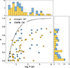 |
Fig. 5. Relationship between period and eccentricity in the OWN sample, compared to other known spectroscopic binaries from the literature. Histograms are also shown. It is noticeable how the OWN SB1 populate the longer periods (log P > 2) and also the largest eccentricities. The continuous curve depicts the upper limit for eccentricity (Moe & Di Stefano 2017). |
There is a remarkable lack of systems with eccentricities higher than e > 0.8. This feature should be interpreted in the context of the dynamical evolution of systems with extreme mass ratios, or possibly those affected by post-supernova processes. Among SB2 systems, some with eccentricities higher than 0.8 are known: HD 93 129 Aa,Ab (Maíz Apellániz et al. 2017, with a large uncertainty for e, but with a confirmed high value for the outer orbit in an incoming paper), HD 101 413 AB (paper II), HD 168 137 Aa,Ab (Le Bouquin et al. 2017), and HD 192 001 (Mahy et al. 2022).
In Fig. 5 we plot the stability limit of Moe & Di Stefano (2017) and we note that two of our systems are close to it, LM Vel and HD 101 205 A. The first one has a compact companion, so the Roche filling criterion should affect only the primary. Nevertheless, at periastron the O star should experience relatively strong tidal forces. The second system, as previously mentioned, is a complex one that requires further study.
The SB1 systems can be divided into “intrinsic SB1” ones, those where the companion is a compact object and no SB2 signal is ever expected (other than from X rays or other signal from the accretion disk), and “temporary SB1” ones, those where we have not detected the companion but expect to do so eventually. Reasons for nondetection of the companion at this point may be lack of coverage or S/N, extreme flux ratios, fast rotation of the secondary, or a combination of those. One way to analyze the possible nature of the companion is to estimate the mass of the primary from its spectrum and assume and inclination of 90° for the orbit and obtaining it from the mass function. We have done that in Fig. 6 obtaining the spectroscopic masses of the primaries from the relationship with spectral type given by Holgado et al. (2025). The histograms in Fig. 6 show that the minimum masses are clearly concentrated in the < 2 M⊙ (low mass for MS stars) and 2–8 M⊙ (intermediate mass for MS stars) regimes. Of the sample in this paper, three systems have minimum companion masses above 10 M⊙ and another three have values close to 8 M⊙ (the limit between intermediate-mass and massive stars). In order of decreasing values, they are as follows:
-
τ CMa Aa,Ab. As mentioned above, the companion of the spectroscopic orbit is a short-period B+B binary composed of two fast rotators. The value of 21.4 M⊙ in Fig. 6 is consistent with that and a high inclination.
-
CPD −5926 00. The companion is seen in our data but we were unable to derive an SB2 orbit despite its minimum mass of 19.2 M⊙.
-
HD 96 946. Slight profile changes between epochs are seen in He Iλ4922 that point to the possible presence of an early-B companion, which would be consistent with the minimum mass of 13.1 M⊙. Further data are needed to confirm it.
-
HD 124 314 Aa,Ab. Sana et al. (2014) detected the companion with interferometry.
-
HD 130 298. As mentioned above, line profile asymmetries were detected, but the results remain inconclusive.
-
HD 152 424. In this case the primary is a supergiant, so it is not surprising that we do not detect the companion due to the expected large flux ratio if it is an early-B dwarf.
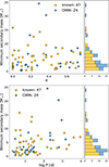 |
Fig. 6. Relationship between eccentricity (top panel), period (bottom panel), and expected minimum mass of the secondary companion in the OWN sample, compared to other known spectroscopic binaries gleaned from the literature. |
In summary, those systems are certain or likely “temporary SB1s”. The only case in our sample where the companion is a compact object for certain is LM Vel and in that case the secondary mass can be as low as 1.3 M⊙.
Data availability
The table containing the RVs of the stars analyzed in this work is available at the CDS via https://cdsarc.cds.unistra.fr/viz-bin/cat/J/A+A/708/A98
Acknowledgments
We thank the anonymous referee for their careful review and valuable comments, which helped improve the quality of this manuscript. R. G. and coauthors from the Instituto de Astrofísica de La Plata acknowledge support from grant PICT 2019-0344 and UNLP G189. We thank the Directors and staff of CASLEO, Las Campanas, La Silla, and Cerro Tololo observatories for the use of their facilities. J. M. A., J. A. M. C., G. H., and S. R. acknowledge support from the Spanish Government Ministerio de Ciencia e Innovación and Agencia Estatal de Investigación (10.13039/501 100 011 033) through grant PID2022-136 640NB-C22 and PID2024-159329NB-C21. G. H. received the support from the “La Caixa” Foundation (ID 100010434) under the fellowship code LCF/BQ/PI23/11970035. S.R. acknowledges support from the Swiss National Funding project 212143. Co-funded by the European Union (Project 101183150 – OCEANS). We are grateful to Lydia Cidale and Ian Thompson for obtaining spectra of HD 152424 during its most recent periastron passage in 2025. OWN data were collected at the European Southern Observatory under ESO programme(s): 077.B-0348(A), 079.D-0564(A), 079.D-0564(B), 079.D-0564(C), 081.D-2008(A), 081.D-2008(B), 083.D-0589(A), 086.D-0997(A), 086.D-0997(B), 087.D-0946(A), 087.D-0946(B), and 089.D-0975(A). Additional LiLiMaRlin data were obtained with the Telescopio Nazionale Galileo, the Nordic Optical Telescope, and the Mercator Telescope at the Observatorio del Roque de los Muchachos (La Palma, Spain); the Very Large Telescope at Observatorio Paranal (Chile); and the 3.6 m and 2.2 m telescopes at Observatorio de La Silla (Chile). NOIRLab IRAF is distributed by the Community Science and Data Center at NSF NOIRLab, which is managed by the Association of Universities for Research in Astronomy (AURA) under a cooperative agreement with the U.S. National Science Foundation. This research has made use of the SIMBAD database, operated at CDS, Strasbourg, France. This research has made use of the NASA Exoplanet Archive, which is operated by the California Institute of Technology, under contract with the National Aeronautics and Space Administration under the Exoplanet Exploration Program. Partially based on observations obtained at the international Gemini Observatory, a program of NSF NOIRLab, which is managed by the Association of Universities for Research in Astronomy (AURA) under a cooperative agreement with the U.S. National Science Foundation on behalf of the Gemini Observatory partnership: the U.S. National Science Foundation (United States), National Research Council (Canada), Agencia Nacional de Investigación y Desarrollo (Chile), Ministerio de Ciencia, Tecnología e Innovación (Argentina), Ministério da Ciência, Tecnologia, Inovações e Comunicações (Brazil), and Korea Astronomy and Space Science Institute (Republic of Korea).
References
- Aldoretta, E. J., Caballero-Nieves, S. M., Gies, D. R., et al. 2015, AJ, 149, 26 [Google Scholar]
- Ansín, T., Gamen, R., Morrell, N. I., et al. 2023, MNRAS, 525, 4566 [CrossRef] [Google Scholar]
- Arias, J. I., Barbá, R. H., Gamen, R. C., et al. 2010, ApJ, 710, L30 [NASA ADS] [CrossRef] [Google Scholar]
- Balona, L. A. 1992, MNRAS, 254, 404 [NASA ADS] [CrossRef] [Google Scholar]
- Barbá, R. H., Gamen, R. C., Arias, J. I., et al. 2010, RMxAC, 38, 30 [Google Scholar]
- Barbá, R. H., Gamen, R., Arias, J. I., & Morrell, N. 2017, IAUS, 329, 89 [Google Scholar]
- Barbá, R. H., Sabín-Sanjulián, C., Arias, J. I., et al. 2020, MNRAS, 494, 3937 [CrossRef] [Google Scholar]
- Bareilles, F. 2017, GBART: Determination of the orbital elements of spectroscopic binaries, Astrophysics Source Code Library [record ascl:1710.014] [Google Scholar]
- Britavskiy, N., Simón-Díaz, S., Holgado, G., et al. 2023, A&A, 672, A22 [NASA ADS] [CrossRef] [EDP Sciences] [Google Scholar]
- Burssens, S., Simón-Díaz, S., Bowman, D. M., et al. 2020, A&A, 639, A81 [NASA ADS] [CrossRef] [EDP Sciences] [Google Scholar]
- Buscombe, W., & Kennedy, P. M. 1969, MNRAS, 143, 1 [Google Scholar]
- Campillay, A. R., Arias, J. I., Barbá, R. H., et al. 2019, MNRAS, 484, 2137 [Google Scholar]
- Chen, X., Liu, Z., & Han, Z. 2024, Prog. Part. Nucl. Phys., 134, 104083 [Google Scholar]
- Chini, R., Hoffmeister, V. H., Nasseri, A., et al. 2012, MNRAS, 424, 1925 [Google Scholar]
- Conti, P. S., Leep, E. M., & Lorre, J. J. 1977, ApJ, 214, 759 [Google Scholar]
- Cruz-González, C., Recillas-Cruz, E., Costero, R., et al. 1974, Rev. Mex. Astron. Astrofis., 1, 211 [Google Scholar]
- Ekström, S. 2021, Front. Astron. Space Sci., 8, 53 [Google Scholar]
- Evans, D. S. 1967, IAU Symp., 30, 57 [NASA ADS] [Google Scholar]
- Feast, M. W., & Thackeray, A. D. 1963, MmRAS, 68, 173 [NASA ADS] [Google Scholar]
- Feast, M. W., Thackeray, A. D., & Wesselink, A. J. 1955, MmRAS, 67, 51 [NASA ADS] [Google Scholar]
- Feast, M. W., Thackeray, A. D., & Wesselink, A. J. 1963, MmRAS, 68, 1 [Google Scholar]
- Fullerton, A. W., Gies, D. R., & Bolton, C. T. 1996, ApJS, 103, 475 [NASA ADS] [CrossRef] [Google Scholar]
- Gamen, R. C., Gosset, E., Morrell, N. I., et al. 2006, A&A, 460, 777 [NASA ADS] [CrossRef] [EDP Sciences] [Google Scholar]
- Gamen, R., Barbá, R., Morrell, N., et al. 2007, BAAA, 50, 105 [Google Scholar]
- Gamen, R. C., Barbá, R. H., Morrell, N. I., Arias, J. I., & Maíz Apellániz, J. 2008a, RMxAC, 33, 54 [Google Scholar]
- Gamen, R. C., Gosset, E., Morrell, N. I., et al. 2008b, RMxAC, 33, 91 [Google Scholar]
- Gamen, R., Barbá, R. H., Walborn, N. R., et al. 2015a, A&A, 583, L4 [NASA ADS] [CrossRef] [EDP Sciences] [Google Scholar]
- Gamen, R., Putkuri, C., Morrell, N. I., et al. 2015b, A&A, 584, A7 [NASA ADS] [CrossRef] [EDP Sciences] [Google Scholar]
- Gaposchkin, S. 1955, MNRAS, 115, 391 [Google Scholar]
- García, B., & Mermilliod, J. C. 2001, A&A, 368, 122 [NASA ADS] [CrossRef] [EDP Sciences] [Google Scholar]
- Garmany, C. D., Conti, P. S., & Massey, P. 1980, ApJ, 242, 1063 [NASA ADS] [CrossRef] [Google Scholar]
- Guo, Y., Liu, C., Wang, L., et al. 2022, A&A, 667, A44 [NASA ADS] [CrossRef] [EDP Sciences] [Google Scholar]
- Hadrava, P. 2004, PAICAS, 92, 1 [Google Scholar]
- Hayes, C. R., Waller, F., Ireland, M., et al. 2022, SPIE Conf. Ser., 12184, 121846H [Google Scholar]
- Hilditch, R. W. 2001, An Introduction to Close Binary Stars (CUP) [Google Scholar]
- Hill, G., Crawford, D. L., & Barnes, J. V. 1974, AJ, 79, 1271 [Google Scholar]
- Holgado, G., Simón-Díaz, S., Barbá, R. H., et al. 2018, A&A, 613, A65 [NASA ADS] [CrossRef] [EDP Sciences] [Google Scholar]
- Holgado, G., Simón-Díaz, S., Haemmerlé, L., et al. 2020, A&A, 638, A157 [NASA ADS] [CrossRef] [EDP Sciences] [Google Scholar]
- Holgado, G., Simón-Díaz, S., Herrero, A., & Barbá, R. H. 2022, A&A, 665, A150 [NASA ADS] [CrossRef] [EDP Sciences] [Google Scholar]
- Holgado, G., Maíz Apellániz, J., & Gamen, R. C. 2025, A&A, 701, A246 [NASA ADS] [CrossRef] [EDP Sciences] [Google Scholar]
- Holgado, G., Simón-Díaz, S., & Herrero, A. 2025, A&A, 703, A175 [NASA ADS] [CrossRef] [EDP Sciences] [Google Scholar]
- Hubrig, S., Schöller, M., Kharchenko, N. V., et al. 2011, A&A, 528, A151 [NASA ADS] [CrossRef] [EDP Sciences] [Google Scholar]
- Ireland, M. J., White, M., Bento, J. P., et al. 2018, SPIE Conf. Ser., 10707, 10 [Google Scholar]
- Labrie, K., Anderson, K., Cárdenes, R., et al. 2019, ASP Conf. Ser. I., 523, 321 [Google Scholar]
- Labrie, K., Simpson, C., Anderson, K., et al. 2022, https://doi.org/10.5281/zenodo.7308726 [Google Scholar]
- Le Bouquin, J. B., Sana, H., Gosset, E., et al. 2017, A&A, 601, A34 [NASA ADS] [CrossRef] [EDP Sciences] [Google Scholar]
- Lefèvre, L., Marchenko, S. V., Moffat, A. F. J., et al. 2009, A&A, 507, 1141 [NASA ADS] [CrossRef] [EDP Sciences] [Google Scholar]
- Levato, H., Morrell, N., Garcia, B., & Malaroda, S. 1988, ApJS, 68, 319 [NASA ADS] [CrossRef] [Google Scholar]
- Levato, H., Malaroda, S., Morrell, N., et al. 1991, ApJS, 75, 869 [NASA ADS] [CrossRef] [Google Scholar]
- Li, L., Zhu, C., Guo, S., Liu, H., & Lü, G. 2023, ApJ, 952, 79 [Google Scholar]
- Lightkurve Collaboration 2018, Lightkurve: Kepler and TESS Time Series Analysis in Python (Astrophysics Source Code Library) [Google Scholar]
- Maeder, A., & Meynet, G. 2000, A&A, 361, 159 [NASA ADS] [Google Scholar]
- Mahy, L., Sana, H., Shenar, T., et al. 2022, A&A, 664, A159 [NASA ADS] [CrossRef] [EDP Sciences] [Google Scholar]
- Maíz Apellániz, J. 2004, in How Does the Galaxy Work?, ASSL, 315, 231 [Google Scholar]
- Maíz Apellániz, J. 2008, ApJ, 677, 1278 [NASA ADS] [CrossRef] [Google Scholar]
- Maíz Apellániz, J., & Barbá, R. H. 2020, A&A, 636, A28 [NASA ADS] [CrossRef] [EDP Sciences] [Google Scholar]
- Maíz Apellániz, J., Sota, A., Walborn, N. R., et al. 2011, HSA, 6, 467 [Google Scholar]
- Maíz Apellániz, J., Pellerin, A., Barbá, R. H., et al. 2012, ASPC, 465, 484 [Google Scholar]
- Maíz Apellániz, J., Sota, A., Arias, J. I., et al. 2016, ApJS, 224, 4 [CrossRef] [Google Scholar]
- Maíz Apellániz, J., Sana, H., Barbá, R. H., et al. 2017, MNRAS, 464, 3561 [CrossRef] [Google Scholar]
- Maíz Apellániz, J., Barbá, R. H., Simón-Díaz, S., et al. 2018a, A&A, 615, A161 [NASA ADS] [CrossRef] [EDP Sciences] [Google Scholar]
- Maíz Apellániz, J., Pantaleoni González, M., Barbá, R. H., et al. 2018b, A&A, 616, A149 [NASA ADS] [CrossRef] [EDP Sciences] [Google Scholar]
- Maíz Apellániz, J., Trigueros Páez, E., Jiménez Martínez, I., et al. 2019a, HSA, 10, 420 [Google Scholar]
- Maíz Apellániz, J., Trigueros Páez, E., Negueruela, I., et al. 2019b, A&A, 626, A20 [NASA ADS] [CrossRef] [EDP Sciences] [Google Scholar]
- Maíz Apellániz, J., Barbá, R. H., Fariña, C., et al. 2021, A&A, 646, A11 [NASA ADS] [CrossRef] [EDP Sciences] [Google Scholar]
- Maíz Apellániz, J., Barbá, R. H., Molina Lera, J. A., et al. 2025, HSA XII, 225 [Google Scholar]
- Maíz Apellániz, J., Negueruela, I., Caballero, José A., et al. 2026, Encycl. Astrophys., 2, 43 [Google Scholar]
- Marraco, H. G., & Muzzio, J. C. 1980, PASP, 92, 700 [Google Scholar]
- Martin, N. 1964, Pub. Obs. Haute-Provence, 7, 33 [Google Scholar]
- Martín-Ravelo, P., Gamen, R., Arias, J. I., et al. 2024, A&A, 690, A306 [NASA ADS] [CrossRef] [EDP Sciences] [Google Scholar]
- Martins, F., Schaerer, D., & Hillier, D. J. 2005, A&A, 436, 1049 [NASA ADS] [CrossRef] [EDP Sciences] [Google Scholar]
- Mason, B. D., Wycoff, G. L., Hartkopf, W. I., et al. 2001, AJ, 122, 3466 [NASA ADS] [CrossRef] [Google Scholar]
- Mayer, P., Lorenz, R., & Drechsel, H. 1992, IBVS, 3765, 1 [Google Scholar]
- Mayer, P., Drechsel, H., & Irrgang, A. 2014, A&A, 565, A86 [NASA ADS] [CrossRef] [EDP Sciences] [Google Scholar]
- Mayer, P., Harmanec, P., Chini, R., et al. 2017, A&A, 600, A33 [NASA ADS] [CrossRef] [EDP Sciences] [Google Scholar]
- McAlister, H., Hartkopf, W. I., & Franz, O. G. 1990, AJ, 99, 965 [Google Scholar]
- Mellon, S. N., Mamajek, E. E., Stuik, R., et al. 2019, ApJS, 244, 15 [NASA ADS] [CrossRef] [Google Scholar]
- Mermilliod, J.-C., & García, B. 2001, IAUS, 200, 191 [Google Scholar]
- Meynet, G., & Maeder, A. 2005, A&A, 429, 581 [CrossRef] [EDP Sciences] [Google Scholar]
- Moe, M., & Di Stefano, R. 2017, ApJS, 230, 15 [Google Scholar]
- Morrell, N. I., Barbá, R. H., Niemela, V. S., et al. 2001, MNRAS, 326, 85 [NASA ADS] [CrossRef] [Google Scholar]
- Neubauer, F. J. 1943, ApJ, 97, 300 [Google Scholar]
- Otero, S. A. 2003, IBVS, 5480, 1 [Google Scholar]
- Pantaleoni González, M., Maíz Apellániz, J., Barbá, R. H., et al. 2021, MNRAS, 504, 2968 [Google Scholar]
- Pantaleoni González, M., Maíz Apellániz, J., Barbá, R. H., et al. 2025, MNRAS, 543, 63 [Google Scholar]
- Pazder, J., et al. 2020, SPIE Conf. Ser., 11447, 1144743 [Google Scholar]
- Perryman, M. A. C., Lindegren, L., Kovalevsky, J., et al. 1997, A&A, 323, L49 [Google Scholar]
- Preibisch, T., Weigelt, G., & Zinnecker, H. 2001, IAUS, 200, 69 [Google Scholar]
- Prusti, T., de Bruijne, J. H. J., Brown, A. G. A., et al. 2016, A&A, 595, A1 [NASA ADS] [CrossRef] [EDP Sciences] [Google Scholar]
- Putkuri, C., Gamen, R., Morrell, N. I., et al. 2021, A&A, 650, A96 [NASA ADS] [CrossRef] [EDP Sciences] [Google Scholar]
- Putkuri, C., Gamen, R., Benvenuto, O. G., et al. 2022, MNRAS, 517, 3101 [Google Scholar]
- Putkuri, C., Gamen, R., Morrell, N. I., et al. 2023, MNRAS, 525, 6084 [NASA ADS] [CrossRef] [Google Scholar]
- Raboud, D. 1996, A&A, 315, 384 [Google Scholar]
- Ricker, G. R., Winn, J. N., Vanderspek, R., et al. 2015, JATIS, 1, 014003 [Google Scholar]
- Rosu, S., Maíz Apellániz, J., Sciarini, L., et al. 2025, arXiv e-prints [arXiv:2510.16202] [Google Scholar]
- Sana, H., de Mink, S. E., de Koter, A., et al. 2012, Science, 337, 444 [Google Scholar]
- Sana, H., de Koter, A., de Mink, S. E., et al. 2013, A&A, 550, A107 [NASA ADS] [CrossRef] [EDP Sciences] [Google Scholar]
- Sana, H., Le Bouquin, J.-B., Lacour, S., et al. 2014, ApJS, 215, 15 [Google Scholar]
- Sanford, R. F. 1949, ApJ, 110, 117 [Google Scholar]
- Sota, A., Maíz Apellániz, J., Morrell, N. I., et al. 2014, ApJS, 211, 10 [Google Scholar]
- Struve, O. 1944, ApJ, 100, 189 [Google Scholar]
- Struve, O., & Pogo, A. 1928, ApJ, 68, 335 [Google Scholar]
- Thackeray, A. D., & Wesselink, A. J. 1965, MNRAS, 131, 121 [Google Scholar]
- Thackeray, A. D., Tritton, S. B., & Walker, E. N. 1973, MmRAS, 77, 199 [NASA ADS] [Google Scholar]
- Tody, D. 1986, in Instrumentation in astronomy VI, ed. D. L. Crawford, SPIE Conf. Ser., 627, 733 [Google Scholar]
- Tody, D. 1993, in Astronomical Data Analysis Software and Systems II, eds. R. J. Hanisch, R. J. V. Brissenden, & J. Barnes, ASP Conf. Ser., 52, 173 [Google Scholar]
- Trigueros Páez, E., Barbá, R. H., Negueruela, I., et al. 2021, A&A, 655, A4 [CrossRef] [Google Scholar]
- van der Hucht, K. A. 2001, NewAR, 45, 135 [NASA ADS] [CrossRef] [Google Scholar]
- van Leeuwen, F., & van Genderen, A. M. 1997, A&A, 327, 1070 [NASA ADS] [Google Scholar]
- Wilson, R. E. 1953, General catalogue of stellar radial velocities (Carnegie Institute Washington D.C. Publication) [Google Scholar]
- Zasche, P., Henzl, Z., & Mašek, M. 2022, A&A, 664, A96 [NASA ADS] [CrossRef] [EDP Sciences] [Google Scholar]
- Zinnecker, H., & Yorke, H. W. 2007, ARA&A, 45, 481 [Google Scholar]
CASLEO is operated under an agreement between CONICET and the National Universities of La Plata, Córdoba, and San Juan, Argentina.
Appendix A: Additional figures and tables
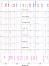 |
Fig. A.1. ALS spectrograms from UNWIND (hence, ISM-free) used for new spectral classifications in this paper. |
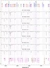 |
Fig. A.2. ALS spectrograms from UNWIND (hence, ISM-free) used for new spectral classifications in this paper. |
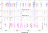 |
Fig. A.3. ALS spectrograms from UNWIND (hence, ISM-free) used for new spectral classifications in this paper. |
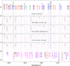 |
Fig. A.4. ALS spectrograms not from UNWIND (hence, with ISM lines) used for new spectral classifications in this paper. |
Spectroscopic orbital elements.
IDs, coordinates, and spectral classifications for the sample in this paper sorted by GOS/GBS ID.
All Tables
IDs, coordinates, and spectral classifications for the sample in this paper sorted by GOS/GBS ID.
All Figures
|
Fig. 1. Stacked histogram of the peak-to-peak RV amplitudes for the 212 targets of the OWN sample, showing the relative contributions of SB1, SB2, RV variables, and constant RV (C) systems. The horizontal scale is logarithmic. |
| In the text | |
|
Fig. 2. Radial velocity curves for OWN targets identified as SB1. Filled circles represent the RVs determined for the primary components. |
| In the text | |
|
Fig. 3. Radial velocity curves for OWN targets identified as SB1. Filled circles represent the RVs determined for the primary components. |
| In the text | |
|
Fig. 4. First panel: Light curve of NX Vel A,B, using the period P = 2.9199 d (only TESS sector 61). Second panel: Same but with the period P = 13.0734 d, obtained from the He II absorption lines. Third panel: Mass-function plot for the NX Vel A spectroscopic orbit. |
| In the text | |
|
Fig. 5. Relationship between period and eccentricity in the OWN sample, compared to other known spectroscopic binaries from the literature. Histograms are also shown. It is noticeable how the OWN SB1 populate the longer periods (log P > 2) and also the largest eccentricities. The continuous curve depicts the upper limit for eccentricity (Moe & Di Stefano 2017). |
| In the text | |
|
Fig. 6. Relationship between eccentricity (top panel), period (bottom panel), and expected minimum mass of the secondary companion in the OWN sample, compared to other known spectroscopic binaries gleaned from the literature. |
| In the text | |
|
Fig. A.1. ALS spectrograms from UNWIND (hence, ISM-free) used for new spectral classifications in this paper. |
| In the text | |
|
Fig. A.2. ALS spectrograms from UNWIND (hence, ISM-free) used for new spectral classifications in this paper. |
| In the text | |
|
Fig. A.3. ALS spectrograms from UNWIND (hence, ISM-free) used for new spectral classifications in this paper. |
| In the text | |
|
Fig. A.4. ALS spectrograms not from UNWIND (hence, with ISM lines) used for new spectral classifications in this paper. |
| In the text | |
Current usage metrics show cumulative count of Article Views (full-text article views including HTML views, PDF and ePub downloads, according to the available data) and Abstracts Views on Vision4Press platform.
Data correspond to usage on the plateform after 2015. The current usage metrics is available 48-96 hours after online publication and is updated daily on week days.
Initial download of the metrics may take a while.