| Issue |
A&A
Volume 708, April 2026
|
|
|---|---|---|
| Article Number | A132 | |
| Number of page(s) | 8 | |
| Section | Numerical methods and codes | |
| DOI | https://doi.org/10.1051/0004-6361/202658902 | |
| Published online | 01 April 2026 | |
A Bayesian framework for astrometry in a sparse star field and its application to Triton observations
1
Department of Computer Science, Jinan University,
Guangzhou
510632,
China
2
School of Mathematics and Computer, Guangdong Ocean University,
Zhanjiang
524088,
China
3
Department of Physics, College of Physics and Optoelectronic Engineering, Jinan University,
Guangzhou
510632,
China
4
Sino-French Joint Laboratory for Astrometry, Dynamics and Space Science, Jinan University,
Guangzhou
510632,
China
★ Corresponding author: This email address is being protected from spambots. You need JavaScript enabled to view it.
Received:
9
January
2026
Accepted:
13
February
2026
Abstract
Context. The Gaia DR3 catalog significantly improves ground-based astrometric precision for natural satellites, largely because sufficient reference stars with high-precision positions are typically available within an object’s field. These stars enable the determination of a high-order plate model (e.g., a fourth-degree polynomial) that can fully absorb the geometric distortion (GD) in the CCD field. However, accurate calibration is still challenging when a natural satellite moves into a small sparse star field (about 12×12 arcmin2) containing only a dozen or so reference stars.
Aims. This study aims to improve natural satellite astrometry in sparse star fields without requiring the calibration observations that are needed for currently well-established GD solutions. Additionally, our previously published observations of Neptune’s largest satellite, Triton, from 2014 to 2016 show a significant positive systematic offset in right ascension, and the underlying reason will be clarified.
Methods. We present a Bayesian framework that models the GD effect using the CCD frames of the science object itself. This approach is self-calibrating and does not require additional calibration observations of dense star fields. The model parameters and their distributions are optimized using the Markov chain Monte Carlo algorithm, and the positional O–C (observed minus computed) values are derived by sampling from these posterior distributions, rather than employing point estimates.
Results. The effectiveness of the proposed approach was evaluated using 985 CCD frames of Triton. The results demonstrate a significant improvement in astrometric precision over the commonly used least-squares (LS) method, and show comparable or even better performance relative to the well-established GD correction method, particularly in the absence of suitable calibration observations. Additionally, we find that the systematic offsets in our previous work on Triton are due to differences in Earth’s precession-nutation theory adopted by the Jet Propulsion Laboratory ephemeris for Triton and adopted by the NOVAS library for reference stars.
Key words: methods: statistical / techniques: image processing / astrometry / planets and satellites: individual: Triton
© The Authors 2026
 Open Access article, published by EDP Sciences, under the terms of the Creative Commons Attribution License (https://creativecommons.org/licenses/by/4.0), which permits unrestricted use, distribution, and reproduction in any medium, provided the original work is properly cited.
This article is published in open access under the Subscribe to Open model. This email address is being protected from spambots. You need JavaScript enabled to view it. to support open access publication.
1 Introduction
High-precision astrometry of natural satellites is essential for refining their orbital models and tidal effects (Lainey et al. 2009), as well as for future space exploration. In recent years, the Gaia catalog releases (Gaia Collaboration 2023b) have revolutionized natural satellites’ ground-based astrometric measurements. The latest Gaia Focused Product Release (FPR) data (Gaia Collaboration 2023a) include observations of 31 planetary satellites1, achieving precision of a few milliarcseconds (mas) for some bright satellites; see Table 3 in Emelyanov et al. (2023) for a reference. However, the data coverage for individual natural satellites is limited due to Gaia’s scanning law and the program object’s motion. Therefore, long-term, high-frequency measurements from ground-based telescopes remain important.
Achieving approximately 10 mas precision for natural satellites in ground-based astrometric measurements necessitates accounting for several major systematic effects, including geometric distortion (GD) of the Charge-Coupled Device (CCD) field, differential color refraction (DCR), and atmospheric turbulence. The DCR effect can be mitigated by observing near the meridian (Ortiz et al. 2017) or by employing a long-wavelength pass-band filter such as Cousins-I (Lin et al. 2020; Fang et al. 2025). The turbulence can be effectively modeled using methods such as Gaussian process regression (Bernstein et al. 2017) or refined precision premium (Zheng et al. 2025), potentially improving precision to better than 10 mas. However, these methods require a large number of stars evenly distributed across the CCD field. A sufficient number of reference stars also aids in solving a high-order plate model (e.g., a fourth-order polynomial) that can fully absorb the GD effect (Ofek 2019; Guo et al. 2022). When a natural satellite moves into a sparse star field, the available number of reference stars (e.g., at least 15 stars for a fourth-order polynomial) may be unsatisfactory. Consequently, we are limited to adopting a first- or second-order plate model, which yields a lower precision since even small CCD fields can exhibit substantial GD effects (Peng & Fan 2010; Peng et al. 2012). In this study we focused on improving precision under such conditions.
At present, the most successful solution is to first derive the GD model using calibration observations of dense star fields instead of the target’s field (Anderson & King 2003; Peng et al. 2012; Zheng et al. 2021), and then applying this derived model to the target’s field. For some historical observations, however, calibration observations are usually unavailable. To address this issue, Lin et al. (2024) propose a method for deriving an analytical GD model without the requirement of dedicated calibration fields. They also demonstrate the overfitting problem of a high-order plate model in sparse star fields where only a dozen bright stars can be used. In contrast to Lin et al. (2024), who adopted a deterministic approach, we investigated this problem from a Bayesian probabilistic perspective, which allowed us to quantify uncertainty and estimate parameter distributions.
In this paper, we utilize observations of Neptune’s largest moon, Triton, to evaluate the effectiveness of our proposed Bayesian framework. Triton has a retrograde, inclined, and circular orbit, suggesting that it may have originally orbited the Sun before being captured by Neptune (Nogueira et al. 2011). These unusual features have motivated many scientists to develop observing campaigns for Triton in recent years (Stone 2001; Wang et al. 2017; Zhang et al. 2021; Yan et al. 2025). Such valuable observations can enhance our understanding of Neptune’s orbit and the evolution of the Solar System.
Another important issue in reducing Triton’s observations from 2014–2016, as reported in our previous work (Wang et al. 2017), is a mean O–C (observed minus computed) offset of approximately 42 mas in right ascension (RA), which is substantial relative to the 12 mas dispersion. Since these previously published observations contributed to the development of the DE440/DE441 ephemerides (see Table 5 in Park et al. 2021) and received attention by other works like Yuan et al. (2025), we intend to re-reduce them. We find that this offset arises from a difference between Earth’s precession-nutation theory2 employed by the Jet Propulsion Laboratory (JPL) and the Naval Observatory Vector Astrometry Software (NOVAS) library (Bangert et al. 2011). This is discussed in Sect. 4.2. The newly reduced topocentric astrometric positions of Triton will be accessible on our website: https://astrometry.jnu.edu.cn/download/list.htm.
The remainder of this paper is organized as follows: Section 2 details the observations of Triton; Sect. 3 introduces the proposed Bayesian framework; Sect. 4 provides the astrometric results of Triton and some discussions; and Sect. 5 concludes the paper.
Specifications of the telescopes and CCD detectors.
2 Observations
We used two datasets of Triton observations. The first set (Set1) comprises 755 CCD observations from 2014 to 2016 and is drawn from our previous work (Wang et al. 2017), with details reported therein. The second set (Set2) comprises 230 CCD observations obtained in 2024 using two ground-based telescopes: a 0.8 m azimuthal-mounted telescope at Yaoan Station, Purple Mountain Observatory (IAU code O49), and a 1 m equatorial-mounted telescope at Yunnan Observatory (IAU code 286). The specifications of both telescopes and their CCD detectors are summarized in Table 1. All Set2 observations were captured using the Cousins-I filter to mitigate the DCR effect. Table A.1 provides an overview of the observations, showing only a few dozen stars in Triton’s field.
The raw CCD frames were initially corrected for bias and flat fielding. Subsequently, a two-dimensional Gaussian function was employed to determine the centroid of star images. Some images of Triton were affected by Neptune’s halo and were pre-processed using a symmetric subtraction procedure (Veiga & Vieira Martins 1995; Xie et al. 2019; Fang et al. 2025).
3 Methods
In a sparse star field with only a dozen or so reference stars, we are often limited to using a linear or second-order plate model, which is not sufficient to accurately account for the GD of the CCD field of view. On the other hand, solving a high-order plate model with the minimum required number of stars (e.g., 15 or slightly more for a fourth-order polynomial) risks overfitting, as observed by Lin et al. (2024). The current most successful practice is to derive the GD model from calibration observations of dense star fields obtained at a different pointing and epoch (assuming the GD model is stable) and apply it to the object’s field; however, such observations may also be unavailable. In this study we assumed that GD remains stable over short periods, such as one or a few nights, and we aimed to combine all science frames within an observing run in order to model the GD effect. Since a star’s centroid can vary between CCD frames (e.g., due to inaccuracies in the telescope’s pointing), changes in the position distribution help ensure the stability of the solved GD model. Before presenting the details of our method, we summarize the characteristics of the traditional least squares (LS) method, the classical geometric distortion correction (GDC) method:
LS: solving a plate model separately for each CCD frame, where the order of the plate model is determined by the number of available stars (Ofek 2019). A second-degree polynomial is applied for fewer than 15 stars, a third-degree for 15 to 25 stars, and a fourth-degree for more than 25 stars.
GDC + LS (linear): the GD model is derived from calibration observations using the method proposed by Peng et al. (2012) and is applied to the object’s field of view. After GDC for pixel coordinates of the reference stars and object, a linear six-parameter plate model is adopted for reduction. For simplicity, this approach is referred to as “GDC” in this paper.
Markov chain Monte Carlo (MCMC): the GD is modeled separately for each observation night by combining all available science frames of an object acquired during that night. For each CCD frame, the displacement, rotation, and scale factor are modeled using a six-parameter plate model, separately, and the GD model is shared across frames. The degree of the GD model is consistent with that in LS, and all parameters are jointly optimized using the MCMC algorithm.
3.1 Observation model
The observation model defines how the celestial coordinates of stars map to the CCD pixel plane. Assuming there is no GD in the field, the i-th star with equatorial coordinates (αi, δi) can be transformed into the pixel coordinates of the m-th exposure using a linear function:
![Mathematical equation: $\[\left\{\begin{array}{l}X_{i, m}=a_m \cdot \xi_i+b_m \cdot \eta_i+c_m \\Y_{i, m}=d_m \cdot \xi_i+e_m \cdot \eta_i+f_m,\end{array}\right.\]$](/articles/aa/full_html/2026/04/aa58902-26/aa58902-26-eq5.png) (1)
(1)
where (ξi, ηi) represent the standard coordinates of star i based on the gnomonic projection. This linear six-parameter model can also account for atmospheric refraction to some extent (Anderson et al. 2006). Next, we model the GD effect using a high-order polynomial:
![Mathematical equation: $\[\left\{\begin{array}{l}\hat{X}_{i, m}=X_{i, m}+\sum_{k+l \leq n} A_{k, l} L_k\left(s \cdot X_{i, m}\right) L_l\left(s \cdot Y_{i, m}\right) \\\hat{Y}_{i, m}=Y_{i, m}+\sum_{k+l \leq n} B_{k, l} L_k\left(s \cdot X_{i, m}\right) L_l\left(s \cdot Y_{i, m}\right),\end{array}\right.\]$](/articles/aa/full_html/2026/04/aa58902-26/aa58902-26-eq6.png) (2)
(2)
where Lk(·) denotes the k-th order Legendre polynomial, Ak,l and Bk,l are coefficients, and s is a fixed factor used to normalize the input to range [−1, 1]. The Legendre polynomials are utilized to ensure numerical stability. All science frames within an observing run can be combined to determine the GD model.
3.2 Optimization and implementation
We constructed our observation model using a Bayesian approach. Given a set of measurements ![Mathematical equation: $\[\mathcal{D}=\left\{\hat{X}_{i, m}, \hat{Y}_{i, m}\right\}\]$](/articles/aa/full_html/2026/04/aa58902-26/aa58902-26-eq7.png) and source coordinates {αi, δi}, we estimated the parameters θ = [am, bm, cm, ..., Ak,l, Bk,l] in Eqs. (1) and (2) by approximating the posterior probability density function:
and source coordinates {αi, δi}, we estimated the parameters θ = [am, bm, cm, ..., Ak,l, Bk,l] in Eqs. (1) and (2) by approximating the posterior probability density function:
![Mathematical equation: $\[\mathcal{P}\left(\theta {\mid} \mathcal{D}, \alpha_i, \delta_i, \ldots\right) \propto \mathcal{P}\left(\mathcal{D} {\mid} \theta, \alpha_i, \delta_i, \ldots\right) \mathcal{P}(\theta),\]$](/articles/aa/full_html/2026/04/aa58902-26/aa58902-26-eq8.png) (3)
(3)
where 𝒫(𝒟|θ, αi, δi, ...) represents the observation model defined in Sect. 3.1 and 𝒫(θ) denotes the prior distributions. For simplicity, we assumed that the measurements for each star follow independent normal distributions. For the six linear parameters (accounting for the scale factor and orientation) in Eq. (1), employing the results from the LS method as initial priors is sufficiently robust; for the GD model, all parameters are assumed to follow a normal distribution, 𝒩(0, 1). There are several important practices to note:
Once the MCMC sampling is complete, we obtain the MCMC chain, from which we estimate the posterior distribution of parameters. For each theoretical position (ξ, η), we draw samples from the posterior via the MCMC chain (e.g., 3000 samples) to get the corresponding (
![Mathematical equation: $\[\hat{X}_{m}, \hat{Y}_{m}\]$](/articles/aa/full_html/2026/04/aa58902-26/aa58902-26-eq9.png) ) values, as detailed in Eqs. (1) and (2). Averaging these values yields the final (
) values, as detailed in Eqs. (1) and (2). Averaging these values yields the final (![Mathematical equation: $\[\hat{X}_{m}, \hat{Y}_{m}\]$](/articles/aa/full_html/2026/04/aa58902-26/aa58902-26-eq10.png) ), which is subsequently used to determine the O–C value.
), which is subsequently used to determine the O–C value.Each observed measurement is assigned an uncertainty level (σi) following the empirical magnitude versus uncertainty relationship described by Lin et al. (2020), establishing a weighting scheme.
The original O–C values are calculated in the pixel plane and need to be projected into standard coordinates, for which a linear six-parameter model is used.
The probabilistic programming was implemented using PyMC3, employing the MCMC algorithm for sampling. Experiments were conducted on a computer equipped with an Intel Core i9-12900K (12th Gen, 3.20 GHz) and an RTX 3070 GPU. Processing 15–30 CCD frames per night takes approximately 1–2 hours. Further processing can integrate observations from multiple successive nights, although this increases the computational time. Figure 1 provides an example of the posterior probability distribution of the parameters, as estimated from observations from November 10, 2024. As shown, the parameters are well estimated, and most parameter pairs exhibit a low linear correlation.
4 Results and discussions
Using observations of Triton, we compared the proposed method with the LS and GDC methods. We employed a weighted scheme as described by Lin et al. (2020). For Set1, the GDC procedure was the same as described in Wang et al. (2017). For Set2, the GD model of the 0.8 m telescope was adopted from Guo et al. (2022), and the GD model of the 1 m telescope was derived from calibration observations obtained on February 22, 2025. Theoretical positions of Triton were retrieved from the JPL ephemerides (DE441+nep097_merged).
4.1 High-precision astrometric positions
We present the O–C residuals for the LS, GDC, and (our) MCMC methods in Figs. 2 and 3. The mean O–C values determined via these methods on different nights are broadly consistent. However, the LS method yields a larger dispersion and a higher incidence of outliers, which may reflect an insufficient distribution of reference stars within the CCD field and potential overfitting. By contrast, the GDC and MCMC methods yield smaller dispersions than LS in both RA and declination (Dec). For Set1, the performance of GDC and our MCMC method is comparable, while for Set2 our MCMC method performs slightly better. This is because Set1 benefits from more calibration observations for deriving GD models on the same date (see Table A.1). However, for Set2, the GD models are derived from a different epoch, which may not be well suited for the science frames.
Table 2 lists the statistics of Triton’s O–C residuals. In Set1, our re-reduced results have a standard deviation closely matching that of our previous work (Wang et al. 2017), i.e., values of approximately 12 mas in each direction. Differences in mean O–C values are likely attributable to updates in the JPL ephemeris and Wang et al. (2017)’s apparent-position-based reduction, which is discussed in Sect. 4.2. In Set2, the standard deviations of observations from the 1 m telescope are somewhat larger than those in Set1, possibly owing to the brighter sky background in 2024 compared with 2014–2016 due to the fact that the city had developed in the intervening period. Observations from the 0.8 m telescope (Site: O49) show larger standard deviations than those from the 1 m telescope (Site: 286), which may be due to the smaller aperture size and shorter exposure time (see Table A.1). Overall, our MCMC method outperforms LS and GDC, with particularly large gains over LS.
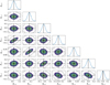 |
Fig. 1 Example of the posterior probability distribution of parameters in the X-direction. The vertical and horizontal lines indicate a mean point estimate, and the subscripts in Ak,l denote the exponent in the X and Y directions, respectively (see also Eq. (2)). |
4.2 Theoretical positions for reduction
In our previous work (Wang et al. 2017), although the standard deviation of the O–C residuals of Triton is small (approximately 12 mas in each direction), a significant positive systematic offset of about 42 mas in the RA direction is evident. Unlike our previous workflows, in this study we used the topocentric astrometric position rather than the topocentric apparent position for relative astrometry reduction. We speculate that the offset arises from differences in the precession-nutation theories employed by JPL (IAU76/80) and NOVAS 3.1 (IAU 2006 precession and IAU 2000A nutation) when computing the apparent positions (Kaplan et al. 1989).
Therefore, we re-reduced Triton’s Set1 observations using topocentric apparent positions and compared the results with those derived from topocentric astrometric positions. Table 3 lists the statistic of Triton’s O–C residuals in Set1 (2014–2016), obtained using the GDC method. As can be seen, compared with the astrometric-position-based results, the apparent-position-based results show a significant positive offset away from the center in the RA directions. The mean O–C difference in RA is about 52 mas, which is in agreement with the −53 mas offset reported by JPL Horizons for the use of IAU76/80 in comparison with IAU 06/00a. Figure 4 illustrates this effect clearly. These results indicate that the astrometric positions are aligned with the JPL ephemeris for Triton and NOVAS for reference stars. If apparent positions are used, care must be taken to ensure the Earth’s precession-nutation theories employed are consistent.
4.3 Strengths and limitations
As demonstrated, our proposed Bayesian approach effectively models the GD effect in the CCD field. While the classical GDC method achieves comparable performance with suitable calibration observations (see the results for Set1), our method performs similarly or somewhat better when such observations are unavailable (see the results for Set2). In other words, our method is self-calibrating because it uses the science frames themselves to model the GD effect, which can reduce biases that can arise if the GD model is derived from observations at a different epoch. In addition, our method estimates the posterior probability distribution of parameters. Each positional O–C value is obtained by drawing samples from these posteriors (see Sect. 3.2 for details). In contrast to the traditional LS method, which relies on point estimates, we can draw a large number of samples from the parameter distribution to obtain more robust estimates (see Figs. 2 and 3).
In this paper, we confine the discussion to a sparse star field within a small CCD field (about 12×12 arcmin2). When a large number of stars (e.g., greater than 100) are evenly distributed in the small CCD field, the traditional LS method can effectively determine a high-order polynomial to absorb the GD effect, and our proposed method may offer only marginal gains in this scenario. On the other hand, our approach employs the MCMC sampling algorithm and requires substantial computational resources and time. On our computer (see also Sect. 3.2), it takes about 1–2 hours to process 15–30 CCD frames. Further exploration of efficiency improvements and the development of practical applications are worthwhile.
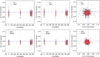 |
Fig. 2 Comparison of the O–C residuals in Set1 (2014–2016). The O–C versus time data points from different methods are slightly shifted to facilitate the comparison. |
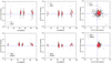 |
Fig. 3 Comparison of the O–C residuals in Set2 (2024). The O–C versus time data points from different methods are slightly shifted to facilitate the comparison. |
Statistics of Triton’s O–C residuals from the three methods.
Statistics of Triton’s O–C residuals using different positions for reduction.
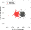 |
Fig. 4 Triton’s O–C residuals in Set1 (2014–2016) using different positions for reduction. |
5 Conclusion
In this paper, we introduce a Bayesian framework for sparse star field astrometry and evaluate its effectiveness using a large dataset of Triton observations. Overall, this approach is comparable to the classical GDC method and significantly improves precision relative to the traditional LS method. We also investigated the origin of a significant positive systematic offset in RA for Triton’s observations from 2014 to 2016, as reported in our previous work (Wang et al. 2017). We find that this offset arises from a difference in the Earth’s precession-nutation theory used by JPL and that used by NOVAS when adopting apparent-position-based reduction procedures.
Acknowledgements
The authors are grateful to the staff at Yunnan Observatory and at Yaoan station of the Purple Mountain Observatory for their assistance throughout our observations. This work was supported by the National Key R&D Program of China (grant no. 2022YFE0116800), by the National Natural Science Foundation of China (grant No. 11873026, 11273014), by the China Manned Space Program (grants no. CMS-CSST-2025-A16, CMS-CSST-2021-B08) and by the Joint Research Fund in Astronomy (grant no. U1431227), by the Natural Science Foundation of Guangdong Province (grant No. 2023A1515011270), by the Scientific Research Starting Foundation of Guangdong Ocean University. This work has made use of data from the European Space Agency (ESA) mission Gaia (https://www.cosmos.esa.int/gaia), processed by the Gaia Data Processing and Analysis Consortium (DPAC, https://www.cosmos.esa.int/web/gaia/dpac/consortium). Funding for the DPAC has been provided by national institutions, in particular the institutions participating in the Gaia Multilateral Agreement.
References
- Anderson, J., & King, I. R. 2003, PASP, 115, 113 [NASA ADS] [CrossRef] [Google Scholar]
- Anderson, J., Bedin, L. R., Piotto, G., Yadav, R. S., & Bellini, A. 2006, A&A, 454, 1029 [NASA ADS] [CrossRef] [EDP Sciences] [Google Scholar]
- Bangert, J., Puatua, W., Kaplan, G., et al. 2011, User’s Guide to NOVAS Version C3.1 (United States Naval Observatory) [Google Scholar]
- Bernstein, G. M., Armstrong, R., Plazas, A. A., et al. 2017, PASP, 129, 074503 [CrossRef] [Google Scholar]
- Emelyanov, N. V., Kovalev, M. Y., & Varfolomeev, M. I. 2023, MNRAS, 522, 165 [NASA ADS] [CrossRef] [Google Scholar]
- Fang, X. Q., Peng, Q. Y., Lu, X., & Guo, B. F. 2025, P&SS, 260, 106085 [Google Scholar]
- Gaia Collaboration (David, P., et al.) 2023a, A&A, 680, A37 [NASA ADS] [CrossRef] [EDP Sciences] [Google Scholar]
- Gaia Collaboration (Vallenari, A., et al.) 2023b, A&A, 674, A1 [NASA ADS] [CrossRef] [EDP Sciences] [Google Scholar]
- Guo, B. F., Peng, Q. Y., Chen, Y., et al. 2022, RAA, 22, 055007 [Google Scholar]
- Kaplan, G. H., Hughes, J., Seidelmann, P., Smith, C., & Yallop, B. 1989, AJ, 97, 1197 [Google Scholar]
- Lainey, V., Arlot, J.-E., Karatekin, Ö., & Van Hoolst, T. 2009, Natur, 459, 957 [Google Scholar]
- Lin, F. R., Peng, Q. Y., & Zheng, Z. J. 2020, MNRAS, 498, 258 [CrossRef] [Google Scholar]
- Lin, F. R., Peng, Q. Y., Zheng, Z. J., & Guo, B. F. 2024, RAA, 24, 115008 [Google Scholar]
- Nogueira, E., Brasser, R., & Gomes, R. 2011, Icar, 214, 113 [Google Scholar]
- Ofek, E. O. 2019, PASP, 131, 054504 [Google Scholar]
- Ortiz, J. L., Santos-Sanz, P., Sicardy, B., et al. 2017, Natur, 550, 219 [Google Scholar]
- Park, R. S., Folkner, W. M., Williams, J. G., & Boggs, D. H. 2021, AJ, 161, 105 [NASA ADS] [CrossRef] [Google Scholar]
- Peng, Q. Y., & Fan, L. Y. 2010, Chi. Sci. Bull., 55, 791 [Google Scholar]
- Peng, Q. Y., Vienne, A., Zhang, Q. F., et al. 2012, AJ, 144, 170 [NASA ADS] [CrossRef] [Google Scholar]
- Stone, R. C. 2001, AJ, 122, 2723 [Google Scholar]
- Veiga, C. H., & Vieira Martins, R. 1995, A&AS, 111, 387 [Google Scholar]
- Wang, N., Peng, Q. Y., Peng, H. W., et al. 2017, MNRAS, 468, 1415 [Google Scholar]
- Xie, H. J., Peng, Q. Y., Wang, N., et al. 2019, P&SS, 165, 110 [Google Scholar]
- Yan, D., Qiao, R. C., Zhang, H. Y., & Yu, Y. 2025, Icar, 116625 [Google Scholar]
- Yuan, Y., Wang, K., Zhu, A., & Li, F. 2025, A&A, 703, A195 [NASA ADS] [CrossRef] [EDP Sciences] [Google Scholar]
- Zhang, H. Y., Qiao, R. C., Yu, Y., Yan, D., & Tang, K. 2021, AJ, 161, 237 [NASA ADS] [CrossRef] [Google Scholar]
- Zheng, Z. J., Peng, Q. Y., & Lin, F. R. 2021, MNRAS, 502, 6216 [CrossRef] [Google Scholar]
- Zheng, Z. J., Peng, Q. Y., Lin, F. R., & Li, D. 2025, AJ, 169, 129 [Google Scholar]
Prior to the publication of this paper, JPL Horizons used the IAU76/80 precession-nutation theory, and the equinox (RA origin) differs by about −53 mas from the IAU2006/00a of-date system employed by NOVAS 3.1. For further details, please refer to https://ssd.jpl.nasa.gov/horizons/manual.html
Appendix A Observations of Triton
Table A.1 provides an overview of the observations of Triton.
Overview of the Triton observations.
All Tables
All Figures
|
Fig. 1 Example of the posterior probability distribution of parameters in the X-direction. The vertical and horizontal lines indicate a mean point estimate, and the subscripts in Ak,l denote the exponent in the X and Y directions, respectively (see also Eq. (2)). |
| In the text | |
|
Fig. 2 Comparison of the O–C residuals in Set1 (2014–2016). The O–C versus time data points from different methods are slightly shifted to facilitate the comparison. |
| In the text | |
|
Fig. 3 Comparison of the O–C residuals in Set2 (2024). The O–C versus time data points from different methods are slightly shifted to facilitate the comparison. |
| In the text | |
|
Fig. 4 Triton’s O–C residuals in Set1 (2014–2016) using different positions for reduction. |
| In the text | |
Current usage metrics show cumulative count of Article Views (full-text article views including HTML views, PDF and ePub downloads, according to the available data) and Abstracts Views on Vision4Press platform.
Data correspond to usage on the plateform after 2015. The current usage metrics is available 48-96 hours after online publication and is updated daily on week days.
Initial download of the metrics may take a while.