| Issue |
A&A
Volume 708, April 2026
|
|
|---|---|---|
| Article Number | A147 | |
| Number of page(s) | 11 | |
| Section | The Sun and the Heliosphere | |
| DOI | https://doi.org/10.1051/0004-6361/202658971 | |
| Published online | 03 April 2026 | |
A data-driven estimate of the protosolar helium mass fraction
1
STAR Institute, Université de Liège, Liège, Belgium
2
Department of Physics, Kurume University, 67 Asahimachi, Kurume, Fukuoka 830-0011, Japan
3
Université Côte d’Azur, Observatoire de la Côte d’Azur, CNRS, Laboratoire Lagrange, Bd de l’Observatoire, CS 34229, 06304 Nice cedex 4, France
4
Centre Spatial de Liège, Université de Liège, Angleur-Liège, Belgium
★ Corresponding author: This email address is being protected from spambots. You need JavaScript enabled to view it.
Received:
15
January
2026
Accepted:
2
March
2026
Abstract
Context. The protosolar helium mass fraction is a fundamental ingredient of solar, planetary models and enrichment laws used to model stellar populations. However, the assumed values often rely on simplifying descriptions of the transport of chemicals in solar models. Furthermore, they are based on the inferred helium mass fraction in the solar convective envelope, which is itself sensitive to uncertainties in the equation of state of the solar material.
Aims. We aim to update the reference protosolar helium abundance by taking into account the effects of macroscopic mixing at the base of the convective zone and using more recent determinations of the helium mass fraction in the convective envelope.
Methods. We combined results from our own inversions of the composition of the solar envelope with spectroscopic abundances, as well as values in the literature, to provide a robust interval of the current helium mass fraction in the convective zone. We combined this measurement with solar models taking into account light element depletion to provide an updated protosolar helium abundance.
Results. We show that macroscopic mixing at the base of the convective envelope of the Sun cannot be neglected to infer the protosolar helium abundance. We demonstrate that as soon as this effect is included, the protosolar helium abundance is significantly reduced and that lithium and beryllium depletion can be used to calibrate this effect over the solar evolution. We find a revised interval of a primordial helium mass fraction of 0.27575 ± 0.00315 slightly lower than previous estimates when combining our latest estimate of the surface helium mass fraction and spectroscopic abundances. We find that the effects of macroscopic mixing are partially compensated by an increase in the inferred solar helium mass fraction in recent studies, but also derive more precise estimates based on various reference works in the literature. If the usual surface helium mass fraction is used, the primordial helium mass fraction drops to 0.2669 ± 0.00415 as a result of the inclusion of macroscopic mixing. The dominant source of uncertainty on this value is found to be the surface helium abundance inferred from helioseismic constraints and, more specifically, the impact on the equation of state of the solar material on this inference result.
Key words: Sun: abundances / Sun: fundamental parameters / Sun: helioseismology / Sun: oscillations
© The Authors 2026
 Open Access article, published by EDP Sciences, under the terms of the Creative Commons Attribution License (https://creativecommons.org/licenses/by/4.0), which permits unrestricted use, distribution, and reproduction in any medium, provided the original work is properly cited.
This article is published in open access under the Subscribe to Open model. This email address is being protected from spambots. You need JavaScript enabled to view it. to support open access publication.
1. Introduction
The protosolar helium abundance, denoted YP, is an important ingredient of planetary models, particularly when simulating the evolution of the giant planets of the Solar System (see e.g. Guillot et al. 1997; Nettelmann et al. 2015; Mankovich et al. 2016; Howard et al. 2024; Nettelmann et al. 2024; Nettelmann & Fortney 2025). Thanks to helioseismology, we are able to estimate the current helium mass fraction in the convective zone (CZ) of the Sun, denoted YCZ (Vorontsov et al. 1991; Basu & Antia 1995; Richard et al. 1998; Di Mauro et al. 2002; Basu & Antia 2004; Vorontsov et al. 2013, 2014; Buldgen et al. 2024a). Each of these studies found a slightly different (though often overlapping at 1σ) value. The most commonly cited is YCZ = 0.24875 ± 0.0035 from Basu & Antia (2004), which is compatible to the value reported by Richard et al. (1998) of YCZ = 0.2480 ± 0.0020. However, these results remain bound to the accuracy of the equation of state of the solar material, and, in practice, the reported values and associated uncertainties may significantly differ (see Sect. 4), as can be seen from the results from Di Mauro et al. (2002)YCZ = 0.2539 ± 0.0005 when using the OPAL equation of state (Rogers et al. 1996; Rogers & Nayfonov 2002) and YCZ = 0.2457 ± 0.0005 when using the magnetohydrodynamic (MHD) equation of state (Hummer & Mihalas 1988; Mihalas et al. 1988; Daeppen et al. 1988; Mihalas et al. 1990). Later studies by Vorontsov et al. (2013) and Vorontsov et al. (2014), combining both OPAL and SAHA-S (Gryaznov et al. 2004, 2006, 2013; Baturin et al. 2013) equations of state, report lower precisions of YCZ = 0.2475 ± 0.0075 and YCZ = 0.2525 ± 0.0075, which are dominated by uncertainties in the equation of state.
The main source of discrepancies between all these studies is the equation of state of the solar plasma, thus motivating continued improvements of the equation of state used in solar and stellar models to achieve higher precision (Antia & Basu 1994; Baturin & Däppen 2003; Trampedach et al. 2006; Baturin et al. 2025; Trampedach & Däppen 2025). All the results above are very consistent with each other, but their respective precision vary significantly, with more recent estimate by Vorontsov et al. (2013) and Vorontsov et al. (2014) being less precise by a factor of two over the usual value taken from Basu & Antia (2004). As we explain below, such a large uncertainty has a direct impact on the protosolar helium mass fraction. To infer the protosolar helium mass fraction, it is necessary to link the current surface helium mass fraction to the protosolar one by assuming and/or simulating the evolution of helium during the life of the Sun. The best way to do this is by computing solar models and analysing the changes in surface composition and its link with the current surface composition of the Sun. Therefore, this relation intrinsically includes a model-dependent dimension through the hypotheses made on the physical ingredients of the solar models, the most straightforward one being mixing prescriptions for chemicals.
Early works by Serenelli & Basu (2010) estimated the protosolar helium abundance from the analysis of a large number of standard solar models (SSMs). They also included some early models simulating turbulence at the base of the solar convective envelope in their work. This work, however, only considered one estimate of the surface helium abundance (Basu & Antia 1995, 2004), which has since been revised using different equations of state (Vorontsov et al. 2013, 2014; Buldgen et al. 2024a) and did not include the depletion of lithium and beryllium in the study of the evolution of the surface helium abundance. However, they considered a 20% uncertainty in microscopic diffusion and related the primordial helium abundance to the surface one using scaling laws from Bahcall (1989). The uncertainties on the treatment of microscopic diffusion have since improved thanks to the full treatment of the effects and extensive comparisons of solar models (Turcotte et al. 1998; Deal et al. 2025). We also refer the reader to Michaud et al. (2015) for a more in-depth discussion on microscopic diffusion.
In this work, we took advantage of the recent determination of lithium ( ) (Wang et al. 2021) and beryllium (
 ) (Amarsi et al. 2024), which are key tracers of the efficiency of the turbulent mixing at the base of the convective zone (BCZ), as these light elements are depleted when compared to meteoritic values,
  and
and  (Lodders 2021). In previous works (Buldgen et al. 2023, 2025a), we showed that including a calibrated mixing efficiency on both elements strongly impacted the initial helium abundance of solar models as well as the conclusions one could draw when comparing solar models to helioseismic constraints. In Deal et al. (2025), we showed that these results were also obtained with various stellar evolution codes and calibration procedures. Using various ingredients that affect the helium mass fraction evolution (opacities, overshooting, nuclear rates) within the same numerical framework, we aim to provide a robust estimation of the primordial helium abundance.
We start in Sect. 2 by discussing the various physical hypotheses that may influence the primordial helium value, separating what concerns the transport of chemicals and other ingredients that will indirectly influence the evolution of the helium mass fraction in the envelope. From this analysis, we can draw an estimate of the difference between the primordial and current envelope helium mass fraction in Sect. 2.2 and finally an estimate of the primordial helium mass fraction in Sect. 4. We conclude by discussing additional improvements to solar models that may help us further increase the precision of this estimate in the coming years.
2. Solar models
In this section we present the properties of the solar models computed with the Liège Stellar Evolution Code (Scuflaire et al. 2008), which we will use to infer the primordial solar helium abundance, YP. We used the AAG21 solar abundances (Asplund et al. 2021), the OPAL (Iglesias & Rogers 1996) and LANL/OPLIB (Colgan et al. 2016) opacities, the mixing-length formalism of convection following Cox & Giuli (1968), the SAHA-S equation of state (version 7), and the NACRE II nuclear reaction rates (Xu et al. 2013). Our models include the Thoul et al. (1994) formalism of diffusion, including the Paquette et al. (1986) screening coefficients, and consider partial ionisation of the chemical elements. Turbulence was treated following Proffitt & Michaud (1991) as in Buldgen et al. (2025a). However, given the similarities found in Buldgen et al. (2025a) and Deal et al. (2025) for other analytical expressions of the empirical turbulent diffusion coefficient, this does not constitute a limitation on the conclusions we draw on turbulence at the BCZ.
The main properties of our solar models are summarised in Table 1, considering first only the effects of turbulent diffusion at the BCZ, and Table 2, where we considered a change of reference opacities, overshooting, and turbulent diffusion. The results for the models considering both the effects of overshooting and turbulent diffusion over a large range of parameters are provided in Table A.1. We used the following naming convention:  implies the inclusion of an additional diffusion coefficient in
  of the following form, as in Proffitt & Michaud (1991):
 (1)
(1)
Global parameters of the solar evolutionary models including turbulent diffusion.
with ρBCZ being the density at the BCZ position and ρ the local density. X and Y are the free parameters in the coefficient that have to be calibrated (usually on light element depletion).
The addition of the suffix ‘LANL’ implies the use of the Los Alamos/OPLIB opacities (Colgan et al. 2016), while ‘Ov Z’ implies the inclusion of overshooting at the BCZ, over a fraction of the local pressure scale height defined by Z, enforcing instantaneous mixing of chemicals and an adiabatic temperature gradient in the overshooting region.
One can already see that directly inferring YP from calibrated solar evolutionary models is not feasible given the interdependences between the physical ingredients of solar models (see e.g. Christensen-Dalsgaard 2021, and refs therein for a recent review). For example, changing the opacity tables in solar models will directly affect YP as a change of opacity in the core of the Sun needs to be compensated such that the solar-calibrated model reproduces the solar luminosity at the solar age (see e.g. Buldgen et al. 2019, for a discussion for a wide range of ingredients of solar models). However, we can already see a crucial element of the evolution of the chemical composition of the solar envelope. Namely, looking at the slope of the values of YCZ, two effects stand out. First, the intensity of turbulence at the BCZ strongly affects the efficiency of settling; for example, in the SSM, the value of YCZ is significantly lower. Second, the physical conditions at the BCZ (e.g. its position, the temperature gradients, etc.) will also slightly affect the helium depletion over time, although on a much smaller scale. Indeed, microscopic diffusion effects are a combination of temperature, pressure, and chemical composition contributions (e.g. Turcotte et al. 1998; Baturin et al. 2006). We illustrate this by plotting the diffusion velocity of helium for three solar models of our sample in Fig. 1.
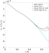 |
Fig. 1. Diffusion velocity of helium for as a function of normalised radius in the radiative zone of solar models (a SSM in light blue and models including macroscopic mixing and/or overshooting at the BCZ in red, green, and purple). |
As can be seen, the presence of turbulence directly affects the diffusion velocity at the BCZ. The differences between the SSM and the model including turbulence from Proffitt & Michaud (1991) go as high as 30%, explaining the observed differences in YCZ at the age of the Sun. This effect is visible even for the lower intensity of turbulent diffusion, even when overshooting is considered, and already well before the models reproduce the lithium and/or beryllium depletion. This implies that such a reduction of the efficiency of microscopic diffusion remains relevant if the uncertainties of the current lithium and beryllium abundances were underestimated.
As it impacts the transport of all elements during the evolution of the Sun, turbulent diffusion at the BCZ has a direct impact on the solar calibration procedure. Indeed, a calibrated solar model must reproduce the solar radius, luminosity, and surface metallicity at the age of the Sun. Due to the effect of turbulence, the evolution of the metals is also impacted, meaning that the initial conditions of the solar calibration are affected by the presence of extra mixing or by variations of the BCZ position. We illustrate this well-known effect in Fig. 2 with the evolution of the surface metallicity, which has been reported in numerous publications (see e.g. Richard et al. 1996; Gabriel 1997; Brun et al. 2002; Christensen-Dalsgaard et al. 2018; Buldgen et al. 2025a). The fact that the BCZ position can be precisely located using helioseismology strongly constrains the allowed variations and, therefore, the impact on the chemical evolution of the position of the convective envelope.
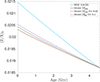 |
Fig. 2. Evolution of surface metallicity of calibrated solar models, (Z/X)S, as a function of time (a SSM in light blue and models including macroscopic mixing and/or overshooting at the BCZ in red, green, and purple). The assumed final metallicity at the solar age is that of Asplund et al. (2021). |
2.1. Impact of light element depletion on the helium mass fraction
Reproducing the observed depletion of lithium and beryllium is a crucial component of the chemical evolution of the Sun and Sun-like stars. While the exact underlying physical mechanism is still unknown, as recent candidates (Eggenberger et al. 2022) were unable to reproduce lithium and beryllium simultaneously (Buldgen et al. 2025a), it is clear that the observed depletion is due to additional mixing occurring at the BCZ. Previous works (Schlattl & Weiss 1999; Zhang et al. 2019) have shown that the depletion of lithium can be reproduced by overshooting, but this process does not induce any beryllium depletion (Kunitomo et al. 2025); it is thus at odds with observations (Amarsi et al. 2024). Results in Eggenberger et al. (2022) also showed that overshooting induced too high a depletion of lithium in young solar twins in open clusters, implying that its impact should be limited. Additionally, Buldgen et al. (2025b) showed that overshooting cannot simultaneously reproduce the properties of the CZ – such as the BCZ position and the height of the entropy plateau in the CZ – while an opacity increase at the BCZ can. These results tend to favour recent hydrodynamical simulations advocating for a limited extent of overshooting at the BCZ. In this context, solar models must reproduce the BCZ position, the entropy plateau height, and the lithium and beryllium depletions simultaneously. Such models can only be produced by assuming ad hoc modifications to the opacity profile and/or additional phenomena or modifications to the physical ingredients (see e.g., amongst others, Guzik et al. 2006; Christensen-Dalsgaard et al. 2009; Serenelli et al. 2009; Ayukov & Baturin 2011, 2017; Buldgen et al. 2019; Zhang et al. 2019; Kunitomo & Guillot 2021; Kunitomo et al. 2022).
Even considering the lithium and beryllium depletions as relatively loose constraints, the overall variation of YCZ, presented in Fig. 3, remains quite similar for a fixed set of physical ingredients. The differences compared to those of an SSM (shown here in red and denoted SSM AAG21) are striking, with a lower YP found in models including turbulence.
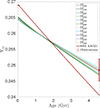 |
Fig. 3. Evolution of helium mass fraction in the convective envelope as a function of time for the models of Table 1. The observed value (red cross) is taken as that of Basu & Antia (2004). |
In Fig. 4 we illustrate the corresponding depletion of lithium and beryllium as a function of time in these models. As mentioned above, we did not consider the lithium and beryllium depletion to be strong constraints and allowed for models in stark disagreement with observations. Nevertheless, even by considering models with significantly lower depletion of light elements then the ones observed, the effect of turbulence of YCZ and YP was immediate. This is a direct consequence of the impact of turbulence on the diffusion velocities, meaning that the snapshot illustrated at the solar age in Fig. 1, where the efficient settling is already damped, happens at much lower efficiencies of turbulent mixing at the BCZ and throughout the evolution of solar models. This demonstrates that the protosolar helium abundance cannot be inferred without considering the impact of turbulence at the BCZ, at it would induce a significant overestimation of its value.
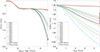 |
Fig. 4. Left panel: Evolution of surface lithium abundance as a function of age (in log scale) for the models of Table 1. The observed value is taken from Wang et al. (2021). Right panel: Evolution of surface beryllium abundance as a function of age (in log scale) for the models of Table 1. The observed value is taken from Amarsi et al. (2024). |
2.2. Importance of the physical ingredients of solar models
As mentioned before, physical ingredients of solar models may play a crucial role. Radiative opacities at high temperatures have a significant impact on YP, with the latest OPLIB opacities leading to a lower value. This change is a direct consequence of a variation of the central temperature of the Sun induced by the intrinsically lower OPLIB opacities in this regime. A similar effect was observed in Ayukov & Baturin (2017) when changing the efficiency of nuclear reactions, or the opacity at high temperatures (see Christensen-Dalsgaard 2021, and refs therein for a detailed discussion). This effect is illustrated in the left panel of Fig. 5, where we can see the evolution of YCZ.
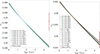 |
Fig. 5. Left panel: Evolution of helium mass fraction in the convective envelope as a function of time for the models of Table 2. The observed value (red cross) is taken as that of Basu & Antia (2004). Right panel: Evolution of helium mass fraction in the convective envelope as a function of time for the models of Table A.1. |
In addition to the effect of a change in opacity, we considered the impact of overshooting at the BCZ. As shown in various publications, adding overshooting leads to an enhanced depletion of lithium, particularly during the pre-main-sequence phase. While this is at odds with young solar twins in open clusters, we still considered the combined impact of overshooting and turbulent diffusion at the BCZ to investigate its potential impact on the evolution of YCZ. If we compare the right panel of Fig. 5 to Fig. 3, we can see that the impact is negligible. In other words, the evolution of the BCZ position under the effect of overshooting has no influence on the depletion of helium, it is solely dominated by turbulence at the BCZ.
In Figs. A.1 and A.2, we also illustrate the evolution of the surface lithium and beryllium abundances as a function of time for the models of Tables A.1 and 2. While the models cover a wide range of final values for both lithium and beryllium, their evolution of YCZ remains similar, implying that the dominant factor is purely the presence of turbulent diffusion at the BCZ. This remains true for a wide range of overshooting values and under the effect of a change of reference opacity tables. Indeed, the only effect of changing the OPAL opacity tables with the OPLIB opacity tables is a vertical shift of YP, which is a simple consequence of the initial conditions of the calibration procedure that requires the calibrated model to reproduce the solar luminosity at the solar age (among other constraints). A direct consequence of the left panel of Fig. 5 is that non-standard models reproducing both lithium and beryllium depletion using the OPLIB opacity tables will not be able to reproduce the YCZ values inferred from helioseismology when using the AAG21 abundances1. The problem is less stringent if a higher solar metallicity is considered (e.g. using the MB22 abundances from Magg et al. 2022); however, as shown in Buldgen et al. (2023) and Buldgen et al. (2024b), a strong disagreement remains with neutrino fluxes, confirming that uncertainties on radiative opacities might not only be an issue at temperatures of the BCZ.
Global parameters of the solar evolutionary models using the OPLIB opacities, including overshooting and turbulent diffusion.
3. Evolution of the helium mass fraction in the convective envelope
As shown in Sect. 2.2, the absolute value of helium abundance in the CZ may vary depending on numerous physical ingredients, but the BCZ position itself has little impact. As already demonstrated in previous works (Serenelli & Basu 2010), the only factors determining the value of YCZ are the initial conditions (thus YP) and the efficiency with which helium settles from the BCZ. In this respect, we emphasise the crucial role of turbulent diffusion at the BCZ in the previous sections. We highlight that it would significantly affect the settling of helium even without considering the current lithium and beryllium abundances as strong constraints in the calibration.
To further illustrate this point, in Figs. 6 and 7 we plot the differences between the initial and primordial helium abundance, YCZ-YP, as a function of time. In all cases, the variation is quite similar and much smaller than the one obtained with an SSM, which is illustrated in the left panel of Fig. 6. The same trend is always obtained, whatever the physical ingredients; the more efficient the turbulent diffusion at the BCZ, the lower the efficiency of settling and the lower the lithium value and beryllium at the age of the Sun. An important point is that the effect of the opacities has been completely erased, as the observed differences, YCZ-YP, for models using OPLIB opacities or OPAL opacities remain well within the same range. This confirms that we can directly infer YP from the knowledge of YCZ and the efficiency of the transport at the BCZ quantified through YCZ-YP at the solar age.
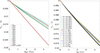 |
Fig. 6. Left panel: Evolution of difference between the protosolar and surface abundance of helium (YCZ-YP) as a function of time for the models of Table 1. Right panel: Same as the left panel but for the models of Table 2. |
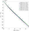 |
Fig. 7. Evolution of difference between the protosolar and surface abundance of helium (YCZ-YP) as a function of time for the models of Table 2. |
From a quantitative point of view, the value YCZ-YP for the SSM is −0.02831, which is very similar to what was found in Serenelli & Basu (2010). As soon as turbulent diffusion is included, considering our entire set of models, this value drops within an interval between −0.01523 and −0.1921. If we consider the lithium and beryllium depletion as strong constraints, this interval further decreases to values between −0.01750 and −0.01888. This means that using an SSM instead of models taking into account light element depletion induces an overestimation of YCZ-YP by about 40%, significantly biasing the estimated protosolar helium abundance.
4. Protosolar helium estimated using the helioseismology of the solar envelope
In this section, we describe how we combined spectroscopic constraints, helioseismic constraints, and the inferred properties of YCZ-YP to recover an updated value of YP. To do this, we made use of the Γ1 inversions of Buldgen et al. (2024a), and more specifically the inferences in the higher part of the convective envelope, from which the helium abundance can be estimated. In Fig. 8, we show an example of an χ2 map used in this work, on which we overlaid the surface area covered when assuming a value of Z/X = 0.0187 ± 0.0009 in agreement with AAG21. In practice, and as shown in Serenelli & Basu (2010), the assumed Z/X has little impact on the inferred YCZ using helioseismic inversions. It may be neglected to first order, but one should keep in mind that some signatures of the partial ionisation of metals in the Γ1 profile are also present at the temperatures where we infer the YCZ value (see e.g. Baturin et al. 2022, for an illustration of the contributions of metals to the Γ1 profile), inducing a small interdependence between the inferred YCZ and ZCZ (the CZ’s metal mass fraction) that can be seen in Vorontsov et al. (2013) and Vorontsov et al. (2014).
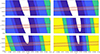 |
Fig. 8. χ2 maps used in Buldgen et al. (2024a) to determine the value of the hydrogen mass fraction as a function of the metal mass fraction in the solar convective envelope. The properties of the models are summarised in their Table 3. The red band shows the range of values compatible with the AAG21 (Z/X)S value. |
In order to perform a rudimentary global analysis, we summarise some YCZ inference results from the literature in Table 3. These values span over three decades of observations, with different instruments, datasets, methods, and equations of state. Overall, the range found is not too different between the various works. However, we can note that the equation of state largely dominates the uncertainty budget in the inference. This underlines the much needed improvements of the solar equation of state as mentioned in Baturin et al. (2025), Trampedach & Däppen (2025).
Helium mass fraction inferred from various groups in the literature.
From our previous work, (Buldgen et al. 2024a) combined with Asplund et al. (2021), we find the following interval for YCZ from our χ2 maps: 0.255 − 0.26. It is in line with the higher values of the results of Vorontsov et al. (2013) and Vorontsov et al. (2014). The main contributor to the uncertainty is again the equation of state, as we considered both SAHA-S (v3 and v7) and FreeEOS (Irwin 2012) for these inferences. It appears that this interval encompasses most of the ones found in Table 3. If we now combine these values to the YCZ-YP differences found in previous sections, we obtain the following result for each YCZ, assuming strong constraints on lithium and beryllium depletion:
-
For Richard et al. (1998): YP = 0.26619 ± 0.00269.
-
For Di Mauro et al. (2002) (MHD): YP = 0.26385 ± 0.00115.
-
For Di Mauro et al. (2002) (OPAL): YP = 0.27205 ± 0.00115.
-
For Basu & Antia (2004): YP = 0.2669 ± 0.00415.
-
For Vorontsov et al. (2013): YP = 0.26565 ± 0.00815.
-
For Vorontsov et al. (2014): YP = 0.27065 ± 0.00815.
-
For this work: YP = 0.27565 ± 0.00315.
A very conservative estimate for YP would fall between 0.2552 and 0.2792, considering the lowest (highest) estimates of YCZ, namely 0.24 and 0.26, combined with the lowest (highest) estimate of YCZ-YP, namely −0.01523 and −0.1921. If we consider only the most recent works and considering the depletion of lithium and beryllium as strong constraints to be achieved by solar models, this interval is reduced to [0.2725,0.2789]. Our value is slightly lower, yet consistent with the interval found by Serenelli & Basu (2010) [0.272,0.284], but for entirely different reasons. In our case, the YCZ is intrinsically higher than theirs due to the YCZ intervals found in the latest analyses, whereas our depletion of helium over time is lower as a result of the inhibition of settling by turbulence at the BCZ.
In fact, had we considered their YCZ and our conservative YCZ-YP values, we would have found YP to be within [0.2605,0.271]. This is even lower than their value estimated from non-SSMs which in their case did not include light element depletion. In all cases, the uncertainties on the YCZ value largely dominate the total budget, with uncertainties on the equation of state dominating the uncertainties on YCZ itself (see e.g. Kosovichev et al. 1992, for an early discussion).
It should also be underlined that the various references provided in Table 3 used different techniques to infer YCZ, as well as different datasets from different instruments. This may give rise to small systematic differences as noted in Basu & Antia (2004) or Buldgen et al. (2024a), the authors of which used revised Michelson Doppler Imager data. Another tedious point is that of surface effect corrections. Apart from the works of Vorontsov et al. (2013) and Vorontsov et al. (2014), all other methods used the individual frequencies directly and thus had to rely on empirical corrections for the surface effects, following, for example, Rabello-Soares et al. (1999) or using a newly derived expression for high-degree modes (Di Mauro et al. 2002). It should also be noted that the differences between Vorontsov et al. (2013) and Vorontsov et al. (2014) stem from different techniques, as the former used two approaches based on the phase shift of frequencies, while the latter used group velocities of the solar acoustic modes. In this context, the uncertainties provided on YCZ are directly related to the ones of the inversion technique, and thus in the case of a given technique mentioned above (such as the SOLA technique in Buldgen et al. 2024a), they only include the propagation of the observational error bars on the frequencies and not other sources of errors.
Therefore, an improvement of YP would also require us to improve the inference of YCZ and carry out a detailed meta-analysis of the overall procedure. In order words, to consistently analyse the impact of various helioseismic datasets, various inference techniques, and equations of state used to determine the value of YCZ, as well as various transport prescriptions (using, e.g. various stellar evolution codes) on the inferred value of YP. Such an analysis is beyond the scope of this work and would only be conclusive if the various equations of state available to solar modellers were to be tested within this framework, using Markov chain Monte Carlo or bootstrap techniques to provide robust uncertainties on the inferred YCZ value.
5. Conclusion
In this study, we analysed the dependences of the inference of the protosolar helium mass fraction, YP, in detail, with the aim of determining an updated value. We show that using SSMs leads to a significant overestimation (by about 40%) of the depletion of helium from the CZ during the solar evolution when compared to solar models reproducing light element depletion. This result is independent of the opacity tables used or of the inclusion of overshooting at the BCZ. We show that the lithium and beryllium abundances at the solar age could serve as efficient calibrators of the efficiency of mixing at the BCZ during the main-sequence evolution of the Sun. Using these constraints, we carried out a meta-analysis of all the values in the literature and inferred an updated interval for YP. A very conservative estimate would be YP = 0.2672 ± 0.012.
When only considering the values for YCZ from Buldgen et al. (2024a) and lithium and beryllium as strong constraints, we find YP = 0.2757 ± 0.0032. This demonstrates the importance of considering the constraints on chemical mixing at the BCZ, as it significantly increases the precision of the inferred YP value.
This value remains consistent with that of Serenelli & Basu (2010) of YP = 0.278 ± 0.006, but this is due to a compensation effect as the YCZ values inferred in recent works is higher than the one from (Basu & Antia 1995) used in Serenelli & Basu (2010). Taking their value of YCZ and remaining conservative on the effects of lithium and beryllium depletion, we find YP = 0.2669 ± 0.00415. This difference underlines the importance of taking into account macroscopic mixing at BCZ, as one cannot assume that SSMs provide an accurate representation of the chemical evolution of the solar convective envelope as they only include microscopic diffusion. The quoted value of YP = 0.2669 ± 0.00415 is perfectly consistent with the value reported in the work of Kunitomo et al. (2025) that used an extended calibration scheme including protosolar accretion and the YCZ value of Basu & Antia (2004) and the OPAL equation of state to describe the solar plasma. It is also noteworthy that protosolar accretion does not affect the inferred value of YP unless the helium mass fraction of the accreted material is significantly different from the protosolar one (such an hypothesis was made in Zhang et al. 2019).
Improving the precision of the inference of YP using solar models first requires us to improve the uncertainties on the YCZ value itself. This requires further improvement of the accuracy of the equation of state of the solar plasma, as it is the main source of uncertainty in the helioseismic inference of YCZ. The second factor influencing the YCZ is the depiction of the outer convective envelope and the so-called surface effect. Limiting their impact by using averaged 3D hydrodynamical simulations instead of grey atmosphere models would bring us closer to resolving the issue. The third limiting factor in the precision of YP is the transport of chemicals at the BCZ. While the physical nature of the macroscopic mixing at the BCZ is unknown, its overall efficiency and impact can still be empirically calibrated using the observed depletion of lithium and beryllium. In this respect, an improved precision on the inference of the current beryllium abundance in the solar photosphere would directly impact our uncertainty on YP. Indeed, the beryllium depletion is an important anchoring point for the efficiency of mixing during the main sequence, while lithium is partially burned during the pre-main sequence.
The above statement does not imply that improvements to the way the transport of chemicals at the BCZ itself is modelled would not significantly increase the precision of the inferred value of YP. A better understanding of the transport of chemicals in the Sun is in any case paramount to improving solar models in general and our inference of stellar ages in light of the requirements of the PLATO mission (Rauer et al. 2025). However, it is likely that the lithium and beryllium depletion will remain crucial observational constraints to confront models with improved transport of chemicals.
Acknowledgments
We thank the referee for their careful reading of the manuscript. GB acknowledges fundings from the Fonds National de la Recherche Scientifique (FNRS) as a postdoctoral researcher. M.K. was supported by JSPS KAKENHI Grant Nos. JP24K00654 and JP24K07099.
References
- Amarsi, A. M., Ogneva, D., Buldgen, G., et al. 2024, A&A, 690, A128 [NASA ADS] [CrossRef] [EDP Sciences] [Google Scholar]
- Antia, H. M., & Basu, S. 1994, ApJ, 426, 801 [Google Scholar]
- Asplund, M., Amarsi, A. M., & Grevesse, N. 2021, A&A, 653, A141 [NASA ADS] [CrossRef] [EDP Sciences] [Google Scholar]
- Ayukov, S. V., & Baturin, V. A. 2011, J. Phys. Conf. Ser., 271, 012033 [NASA ADS] [CrossRef] [Google Scholar]
- Ayukov, S. V., & Baturin, V. A. 2017, Astron. Rep., 61, 901 [NASA ADS] [CrossRef] [Google Scholar]
- Bahcall, J. N. 1989, Neutrino Astrophysics [Google Scholar]
- Basu, S., & Antia, H. M. 1995, MNRAS, 276, 1402 [NASA ADS] [Google Scholar]
- Basu, S., & Antia, H. M. 2004, ApJ, 606, L85 [CrossRef] [Google Scholar]
- Baturin, V. A., & Däppen, W. 2003, Astron. Rep., 47, 685 [Google Scholar]
- Baturin, V. A., Gorshkov, A. B., & Ayukov, S. V. 2006, Astron. Rep., 50, 1001 [NASA ADS] [CrossRef] [Google Scholar]
- Baturin, V. A., Ayukov, S. V., Gryaznov, V. K., et al. 2013, ASP Conf. Ser., 479, 11 [NASA ADS] [Google Scholar]
- Baturin, V. A., Oreshina, A. V., Däppen, W., et al. 2022, A&A, 660, A125 [NASA ADS] [CrossRef] [EDP Sciences] [Google Scholar]
- Baturin, V. A., Ayukov, S. V., Oreshina, A. V., et al. 2025, Sol. Phys., 300, 3 [Google Scholar]
- Brun, A. S., Antia, H. M., Chitre, S. M., & Zahn, J.-P. 2002, A&A, 391, 725 [NASA ADS] [CrossRef] [EDP Sciences] [Google Scholar]
- Buldgen, G., Salmon, S. J. A. J., Noels, A., et al. 2019, A&A, 621, A33 [NASA ADS] [CrossRef] [EDP Sciences] [Google Scholar]
- Buldgen, G., Eggenberger, P., Noels, A., et al. 2023, A&A, 669, L9 [NASA ADS] [CrossRef] [EDP Sciences] [Google Scholar]
- Buldgen, G., Noels, A., Baturin, V. A., et al. 2024a, A&A, 681, A57 [NASA ADS] [CrossRef] [EDP Sciences] [Google Scholar]
- Buldgen, G., Noels, A., Scuflaire, R., et al. 2024b, A&A, 686, A108 [NASA ADS] [CrossRef] [EDP Sciences] [Google Scholar]
- Buldgen, G., Noels, A., Amarsi, A. M., et al. 2025a, A&A, 694, A285 [NASA ADS] [CrossRef] [EDP Sciences] [Google Scholar]
- Buldgen, G., Noels, A., Baturin, V. A., et al. 2025b, A&A, 700, A50 [NASA ADS] [CrossRef] [EDP Sciences] [Google Scholar]
- Christensen-Dalsgaard, J. 2021, Liv. Rev. Sol. Phys., 18, 2 [NASA ADS] [CrossRef] [Google Scholar]
- Christensen-Dalsgaard, J., di Mauro, M. P., Houdek, G., & Pijpers, F. 2009, A&A, 494, 205 [NASA ADS] [CrossRef] [EDP Sciences] [Google Scholar]
- Christensen-Dalsgaard, J., Gough, D. O., & Knudstrup, E. 2018, MNRAS, 477, 3845 [CrossRef] [Google Scholar]
- Colgan, J., Kilcrease, D. P., Magee, N. H., et al. 2016, ApJ, 817, 116 [Google Scholar]
- Cox, J. P., & Giuli, R. T. 1968, Principles of Stellar Structure (Gordon and Breach) [Google Scholar]
- Daeppen, W., Mihalas, D., Hummer, D. G., & Mihalas, B. W. 1988, ApJ, 332, 261 [NASA ADS] [CrossRef] [Google Scholar]
- Deal, M., Buldgen, G., Manchon, L., et al. 2025, Sol. Phys., 300, 96 [Google Scholar]
- Di Mauro, M. P., Christensen-Dalsgaard, J., Rabello-Soares, M. C., & Basu, S. 2002, A&A, 384, 666 [NASA ADS] [CrossRef] [EDP Sciences] [Google Scholar]
- Eggenberger, P., Buldgen, G., Salmon, S. J. A. J., et al. 2022, Nat. Astron., 6, 788 [NASA ADS] [CrossRef] [Google Scholar]
- Gabriel, M. 1997, A&A, 327, 771 [Google Scholar]
- Gryaznov, V. K., Ayukov, S. V., Baturin, V. A., et al. 2004, AIP Conf. Ser., 731, 147 [NASA ADS] [CrossRef] [Google Scholar]
- Gryaznov, V. K., Ayukov, S. V., Baturin, V. A., et al. 2006, J. Phys. A Math. Gen., 39, 4459 [NASA ADS] [CrossRef] [Google Scholar]
- Gryaznov, V. K., Iosilevskiy, I. L., Fortov, V. E., et al. 2013, Contrib. Plasma Phys., 53, 392 [NASA ADS] [CrossRef] [Google Scholar]
- Guillot, T., Gautier, D., & Hubbard, W. B. 1997, Icarus, 130, 534 [Google Scholar]
- Guzik, J. A., Watson, L. S., & Cox, A. N. 2006, Mem. Soc. Astron. It., 77, 389 [NASA ADS] [Google Scholar]
- Howard, S., Müller, S., & Helled, R. 2024, A&A, 689, A15 [NASA ADS] [CrossRef] [EDP Sciences] [Google Scholar]
- Hummer, D. G., & Mihalas, D. 1988, ApJ, 331, 794 [NASA ADS] [CrossRef] [Google Scholar]
- Iglesias, C. A., & Rogers, F. J. 1996, ApJ, 464, 943 [NASA ADS] [CrossRef] [Google Scholar]
- Irwin, A. W. 2012, Astrophysics Source Code Library [record ascl:1211.002] [Google Scholar]
- Kosovichev, A. G., Christensen-Dalsgaard, J., Daeppen, W., et al. 1992, MNRAS, 259, 536 [NASA ADS] [CrossRef] [Google Scholar]
- Kunitomo, M., & Guillot, T. 2021, A&A, 655, A51 [NASA ADS] [CrossRef] [EDP Sciences] [Google Scholar]
- Kunitomo, M., Guillot, T., & Buldgen, G. 2022, A&A, 667, L2 [NASA ADS] [CrossRef] [EDP Sciences] [Google Scholar]
- Kunitomo, M., Buldgen, G., & Guillot, T. 2025, A&A, 702, A167 [NASA ADS] [CrossRef] [EDP Sciences] [Google Scholar]
- Lodders, K. 2021, Space Sci. Rev., 217, 44 [NASA ADS] [CrossRef] [Google Scholar]
- Magg, E., Bergemann, M., Serenelli, A., et al. 2022, A&A, 661, A140 [NASA ADS] [CrossRef] [EDP Sciences] [Google Scholar]
- Mankovich, C., Fortney, J. J., & Moore, K. L. 2016, ApJ, 832, 113 [NASA ADS] [CrossRef] [Google Scholar]
- Michaud, G., Alecian, G., & Richer, J. 2015, Atomic Diffusion in Stars [Google Scholar]
- Mihalas, D., Dappen, W., & Hummer, D. G. 1988, ApJ, 331, 815 [NASA ADS] [CrossRef] [Google Scholar]
- Mihalas, D., Hummer, D. G., Mihalas, B. W., & Daeppen, W. 1990, ApJ, 350, 300 [NASA ADS] [CrossRef] [Google Scholar]
- Nettelmann, N., & Fortney, J. J. 2025, Planet. Sci. J., 6, 98 [Google Scholar]
- Nettelmann, N., Fortney, J. J., Moore, K., & Mankovich, C. 2015, MNRAS, 447, 3422 [NASA ADS] [CrossRef] [Google Scholar]
- Nettelmann, N., Cano Amoros, M., Tosi, N., Helled, R., & Fortney, J. J. 2024, Space Sci. Rev., 220, 56 [CrossRef] [Google Scholar]
- Paquette, C., Pelletier, C., Fontaine, G., & Michaud, G. 1986, ApJS, 61, 177 [Google Scholar]
- Proffitt, C. R., & Michaud, G. 1991, ApJ, 380, 238 [Google Scholar]
- Rabello-Soares, M. C., Basu, S., & Christensen-Dalsgaard, J. 1999, MNRAS, 309, 35 [NASA ADS] [CrossRef] [Google Scholar]
- Rauer, H., Aerts, C., Cabrera, J., et al. 2025, Exp. Astron., 59, 26 [Google Scholar]
- Richard, O., Vauclair, S., Charbonnel, C., & Dziembowski, W. A. 1996, A&A, 312, 1000 [NASA ADS] [Google Scholar]
- Richard, O., Dziembowski, W. A., Sienkiewicz, R., & Goode, P. R. 1998, A&A, 338, 756 [NASA ADS] [Google Scholar]
- Rogers, F. J., & Nayfonov, A. 2002, ApJ, 576, 1064 [Google Scholar]
- Rogers, F. J., Swenson, F. J., & Iglesias, C. A. 1996, ApJ, 456, 902 [Google Scholar]
- Schlattl, H., & Weiss, A. 1999, A&A, 347, 272 [NASA ADS] [Google Scholar]
- Scuflaire, R., Théado, S., Montalbán, J., et al. 2008, ApSS, 316, 83 [NASA ADS] [Google Scholar]
- Serenelli, A. M., & Basu, S. 2010, ApJ, 719, 865 [NASA ADS] [CrossRef] [Google Scholar]
- Serenelli, A. M., Basu, S., Ferguson, J. W., & Asplund, M. 2009, ApJ, 705, L123 [Google Scholar]
- Thoul, A. A., Bahcall, J. N., & Loeb, A. 1994, ApJ, 421, 828 [Google Scholar]
- Trampedach, R., & Däppen, W. 2025, Sol. Phys., 300, 7 [Google Scholar]
- Trampedach, R., Däppen, W., & Baturin, V. A. 2006, ApJ, 646, 560 [NASA ADS] [CrossRef] [Google Scholar]
- Turcotte, S., Richer, J., Michaud, G., Iglesias, C. A., & Rogers, F. J. 1998, ApJ, 504, 539 [Google Scholar]
- Vorontsov, S. V., Baturin, V. A., & Pamiatnykh, A. A. 1991, Nature, 349, 49 [Google Scholar]
- Vorontsov, S. V., Baturin, V. A., Ayukov, S. V., & Gryaznov, V. K. 2013, MNRAS, 430, 1636 [Google Scholar]
- Vorontsov, S. V., Baturin, V. A., Ayukov, S. V., & Gryaznov, V. K. 2014, MNRAS, 441, 3296 [NASA ADS] [CrossRef] [Google Scholar]
- Wang, E. X., Nordlander, T., Asplund, M., et al. 2021, MNRAS, 500, 2159 [Google Scholar]
- Xu, Y., Takahashi, K., Goriely, S., et al. 2013, Nucl. Phys. A, 918, 61 [Google Scholar]
- Zhang, Q.-S., Li, Y., & Christensen-Dalsgaard, J. 2019, ApJ, 881, 103 [Google Scholar]
This issue has already been discussed extensively in Buldgen et al. (2019) for a wide variety of physical ingredients.
Appendix A: Additional table and figures
We provide in Table A.1 the fundamental parameters of our models including both overshooting and turbulent diffusive mixing at the BCZ. We illustrate in Figs. A.1 and A.2 the lithium and beryllium depletion of our models including overshooting at the BCZ and using the Los Alamos opacities instead of the OPAL opacities. The mixing efficiencies and overshooting values are varied far beyond what would be considered reasonable regarding light element depletion.
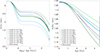 |
Fig. A.1. Left panel: Evolution of surface Lithium abundance as a function of age (in log scale) for the models of Table 2. The ‘Observed’ value is taken from Wang et al. (2021). Right panel: Evolution of the surface Beryllium abundance as a function of age (in log scale) for the models of Table 2. The “Observed” value is taken from Amarsi et al. (2024). |
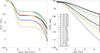 |
Fig. A.2. Left panel: Evolution of surface Lithium abundance as a function of age (in log scale) for the models of Table A.1. The ‘Observed’ value is taken from Wang et al. (2021). Right panel: Evolution of the surface Beryllium abundance as a function of age (in log scale) for the models of Table A.1. The “Observed” value is taken from Amarsi et al. (2024). |
Global parameters of the solar evolutionary models including overshooting and turbulent diffusion.
All Tables
Global parameters of the solar evolutionary models including turbulent diffusion.
Global parameters of the solar evolutionary models using the OPLIB opacities, including overshooting and turbulent diffusion.
Global parameters of the solar evolutionary models including overshooting and turbulent diffusion.
All Figures
|
Fig. 1. Diffusion velocity of helium for as a function of normalised radius in the radiative zone of solar models (a SSM in light blue and models including macroscopic mixing and/or overshooting at the BCZ in red, green, and purple). |
| In the text | |
|
Fig. 2. Evolution of surface metallicity of calibrated solar models, (Z/X)S, as a function of time (a SSM in light blue and models including macroscopic mixing and/or overshooting at the BCZ in red, green, and purple). The assumed final metallicity at the solar age is that of Asplund et al. (2021). |
| In the text | |
|
Fig. 3. Evolution of helium mass fraction in the convective envelope as a function of time for the models of Table 1. The observed value (red cross) is taken as that of Basu & Antia (2004). |
| In the text | |
|
Fig. 4. Left panel: Evolution of surface lithium abundance as a function of age (in log scale) for the models of Table 1. The observed value is taken from Wang et al. (2021). Right panel: Evolution of surface beryllium abundance as a function of age (in log scale) for the models of Table 1. The observed value is taken from Amarsi et al. (2024). |
| In the text | |
|
Fig. 5. Left panel: Evolution of helium mass fraction in the convective envelope as a function of time for the models of Table 2. The observed value (red cross) is taken as that of Basu & Antia (2004). Right panel: Evolution of helium mass fraction in the convective envelope as a function of time for the models of Table A.1. |
| In the text | |
|
Fig. 6. Left panel: Evolution of difference between the protosolar and surface abundance of helium (YCZ-YP) as a function of time for the models of Table 1. Right panel: Same as the left panel but for the models of Table 2. |
| In the text | |
|
Fig. 7. Evolution of difference between the protosolar and surface abundance of helium (YCZ-YP) as a function of time for the models of Table 2. |
| In the text | |
|
Fig. 8. χ2 maps used in Buldgen et al. (2024a) to determine the value of the hydrogen mass fraction as a function of the metal mass fraction in the solar convective envelope. The properties of the models are summarised in their Table 3. The red band shows the range of values compatible with the AAG21 (Z/X)S value. |
| In the text | |
|
Fig. A.1. Left panel: Evolution of surface Lithium abundance as a function of age (in log scale) for the models of Table 2. The ‘Observed’ value is taken from Wang et al. (2021). Right panel: Evolution of the surface Beryllium abundance as a function of age (in log scale) for the models of Table 2. The “Observed” value is taken from Amarsi et al. (2024). |
| In the text | |
|
Fig. A.2. Left panel: Evolution of surface Lithium abundance as a function of age (in log scale) for the models of Table A.1. The ‘Observed’ value is taken from Wang et al. (2021). Right panel: Evolution of the surface Beryllium abundance as a function of age (in log scale) for the models of Table A.1. The “Observed” value is taken from Amarsi et al. (2024). |
| In the text | |
Current usage metrics show cumulative count of Article Views (full-text article views including HTML views, PDF and ePub downloads, according to the available data) and Abstracts Views on Vision4Press platform.
Data correspond to usage on the plateform after 2015. The current usage metrics is available 48-96 hours after online publication and is updated daily on week days.
Initial download of the metrics may take a while.