| Issue |
A&A
Volume 708, April 2026
|
|
|---|---|---|
| Article Number | A24 | |
| Number of page(s) | 5 | |
| Section | Astrophysical processes | |
| DOI | https://doi.org/10.1051/0004-6361/202659052 | |
| Published online | 26 March 2026 | |
Optimising the global detection of solar-like oscillations
Tuning the frequency range for asteroseismic detection predictions and searches
1
Stellar Astrophysics Centre, Department of Physics and Astronomy, Aarhus University, Ny Munkegade 120, DK-8000 Aarhus C, Denmark
2
School of Physics and Astronomy, University of Birmingham, Birmingham B15 2TT, United Kingdom
★ Corresponding authors: This email address is being protected from spambots. You need JavaScript enabled to view it.
; This email address is being protected from spambots. You need JavaScript enabled to view it.
Received:
20
January
2026
Accepted:
3
March
2026
Abstract
Context. A well-established method exists for predicting the detectability of solar-like oscillations that has seen extensive application supporting target selection strategies for space-based photometric missions. The method assesses the probability of making an asteroseismic detection based on the expected global signal-to-noise ratio (SNR) of the observed signal due to the oscillations against the broadband background due to shot noise and granulation. Known stellar parameters are used to compute the expected oscillation and granulation signal, while instrumental specifications and the apparent brightness of the target are used to compute the expected shot noise.
Aims. We explore whether there is an optimal choice for the range in frequency, W, over which the global SNR is determined. The observed power in solar-like oscillations is assumed to follow a Gaussian-like envelope of the full width at half maximum Γenv, centred on the frequency of maximum oscillation power. It has been common practice to set W ≃ 2Γenv when predicting detections.
Methods. We make numerical predictions of the global SNR and resulting detection probabilities for a range of underlying stellar and observational parameters, adopting different choices for the width using W = αΓenv, where α is a multiplicative coefficient that controls the width. We also explored the effect of this choice on detection yields across an ensemble of targets, using a sample of bright solar-like oscillators observed by TESS as a representative example.
Results. We found that the commonly adopted value of α ≃ 2 is a sub-optimal choice and that adopting a range with α ≃ 1.2 maximises the detection probability. There can also be a substantial effect on the predicted detection yield across a sample of stars.
Conclusions. In summary, we recommend the adoption of a range W ≃ 1.2Γenv, not only in computations of the detection probabilities, but also in actual searches for oscillations in real data based on testing the significance of excess mode power, since its adoption will also optimise the probability of making robust detections.
Key words: asteroseismology / methods: statistical / stars: late-type / stars: oscillations
© The Authors 2026
 Open Access article, published by EDP Sciences, under the terms of the Creative Commons Attribution License (https://creativecommons.org/licenses/by/4.0), which permits unrestricted use, distribution, and reproduction in any medium, provided the original work is properly cited.
This article is published in open access under the Subscribe to Open model. This email address is being protected from spambots. You need JavaScript enabled to view it. to support open access publication.
1. Introduction
Solar-like oscillations have now been detected in hundreds of cool main-sequence and subgiant stars and in thousands of red giants (e.g. see Chaplin & Miglio 2013; García & Ballot 2019). Because the oscillation parameters follow scaling relations that depend on fundamental stellar properties to a very good approximation (e.g. see Basu & Chaplin 2017), it is possible to make straightforward predictions of the detectability of the oscillations if the noise budget of the observations is known and to use these known characteristics to tune codes that seek to detect signatures of oscillations in the data. The ability to make such predictions is central to target selection strategies, in particular those for space-based photometric missions. It can inform decisions on the selection of observing fields, specific targets, and observing durations, and so on in order to fulfil mission-specific requirements on detection yields that support specific science goals.
We present an optimisation of the detection prediction method of Chaplin et al. (2011). This approach was developed to inform asteroseismic target selection strategies for the NASA Kepler mission, and has since been used for the K2 (Chaplin et al. 2015; Lund et al. 2016, 2024), the Transiting Exoplanet Survey Satellite (TESS) (Campante et al. 2016; Schofield et al. 2019; Hey et al. 2024), and the CHaracterising ExOPlanet Satellite (CHEOPS) (Moya et al. 2018) missions, and more recently, in preparations for the upcoming ESA PLAnetary Transits and Oscillations of stars (PLATO) mission (Goupil et al. 2024). The optimisation is of the choice of frequency range over which to calculate the global signal-to-noise ratio (SNR) of the oscillations in the frequency power spectrum of the data. This optimal choice of range is then also relevant to the actual searches for oscillations in real data, since its adoption optimises the probability of making robust detections.
The layout of the rest of the paper is as follows. In Sect. 2 we recapitulate the key elements of the method. Sect. 3 contains the main results of the paper. Sect. 3.1 presents formulae to describe the integrated oscillations power and global SNR over different ranges in frequency. We then use these formulae in Sect. 3.2 to show that the commonly adopted choice of frequency range is sub-optimal, and we provide updated guidance on the best range to adopt in detection predictions and in actual searches for the oscillations. We present our main conclusions in Sect. 4.
2. The detection recipe
We begin by summarising the key elements of the Chaplin et al. (2011) approach. First, we followed the well-established convention of assuming that when smoothed in frequency, the observed power in solar-like oscillations follows a Gaussian-like envelope centred on the frequency of maximum oscillation power, νmax. We may then write the power spectral density P(ν) of the envelope as
![Mathematical equation: $$ \begin{aligned} P(\nu ) = H_{\rm env} \exp \!\left[ -\,4\ln 2 \left( \frac{\nu - \nu _{\max }}{\Gamma _{\rm env}} \right)^2 \right], \end{aligned} $$](/articles/aa/full_html/2026/04/aa59052-26/aa59052-26-eq1.gif) (1)
(1)
where Henv and Γenv are the height and full width at half maximum (FWHM) of the envelope, respectively. The total area below the envelope corresponds to the total detected mean-square power in the oscillations and is given by (e.g. see Basu & Chaplin 2017)
 (2)
(2)
The height of the envelope is, in turn, given by
 (3)
(3)
where Amax is the RMS maximum equivalent radial mode amplitude, Δν is the large frequency separation, and ς is the sum of the mode visibilities in power, that is, the sum over l = 0, 1, 2, and 3 in each order, normalised to unity for l = 0. The width of the envelope was assumed to take the form (e.g. see Mosser et al. 2010, 2012; Chaplin et al. 2011)
 (4)
(4)
where α and β are coefficients. Combining the above gives
 (5)
(5)
Predictions of Ptot may be made for a given stellar target using well-established scaling relations for the oscillation parameters (e.g. see Basu & Chaplin 2017 for further details).
The Chaplin et al. (2011) detection method then uses the global SNR in the oscillations, as defined by
 (6)
(6)
where Btot is the total background power across the frequency range occupied by the modes. In what follows, we denote this range as W.
The background has contributions from shot and other instrumental noise, as well as from stellar granulation. We assumed that the underlying limit spectra arising from the combination of background sources, that is, the spectra that would be given by an infinite number of realisations of the data, vary slowly or are approximately constant across the frequency range of interest. The larger the shot-noise contribution, the more the background power spectral density will tend to be flat in frequency, because this white contribution will then dominate the frequency-dependent granulation term. In practice, ignoring the frequency dependence of the background does not significantly affect the detection probability calculation (Chaplin et al. 2011).
We then specified an average background power spectral density  , from which it follows that
 (7)
(7)
Estimates of the noise will depend on the apparent brightness of the target, the instrumental response, and the sensitivity; while the granulation contribution is computed at νmax using scaling relations that depend on fundamental stellar properties (Kallinger et al. 2014; Larsen et al. 2026).
When the time-domain observations span a duration T, the number of independent frequency bins N in the range W is
 (8)
(8)
The power spectral density within any independent bin will follow χ2 2 d.o.f. statistics about the underlying limit spectrum (Appourchaux 2014). The global SNR, which is computed over N bins, then follows χ2 2N d.o.f. statistics. With predicted estimates of the underlying Ptot and total noise Btot in hand for a particular target, we may then calculate the probability pfinal that the observed SNR would exceed some false-alarm threshold pfalse, consistent with the statistics defined above (Appourchaux 2004).
Whilst the various implementations of the Chaplin et al. (2011) detection procedure (i.e. in Campante et al. 2016; Moya et al. 2018; Schofield et al. 2019; Hey et al. 2024; Goupil et al. 2024) have made varying assumptions about how Γenv scales with νmax, they all followed the practice of setting W ≃ 2Γenv, so that the full range encompasses most (strictly, just over 95%) of the total oscillation power Ptot. We proceed below to show that this is a sub-optimal choice.
3. Optimisation of the full range W
3.1. Generalised formulae for different ranges W
To test how the global SNR and detection probability pfinal depend on the choice of range W, we begin by presenting formulae that capture differing fractions of the full Gaussian envelope. We define a coefficient α that controls the range according to
 (9)
(9)
Previous practice has therefore been consistent with setting α ≃ 2.
The integrated area of the Gaussian envelope contained within a symmetric frequency range W about νmax is
 (10)
(10)
Evaluating the integral gives
 (11)
(11)
where Ptot is the full Gaussian area given by Eq. (2). We may rewrite the error function (erf) in the above in terms of α alone (compare Eq. (9)), and changing the independent variable specifying the dependence of the integral on the selected range from W to α, we have
 (12)
(12)
The global SNR is
 (13)
(13)
which we may write explicitly as
 (14)
(14)
To help understand the results that follow, it is also instructive to express the formulae in terms of an average power spectral density  across the range defined by α, that is,
 (15)
(15)
The global SNR may then be written in the form
 (16)
(16)
from which it is clear that it scales directly with the average power spectral density.
It is obvious that by increasing α, and hence W, the average power spectral density  and the global SNR will decrease. However, this must be compared against the commensurate increase in N, and hence, the number of degrees of freedom governing the statistics of the global SNR. At fixed SNR, the larger N, the higher the detection probability pfinal. In short, the SNR required for a detection will be reduced. The combination of these opposing effects suggests that there will be an optimal choice for α that provides the best compromise.
3.2. The optimal frequency range
The left panel of Fig. 1 shows the variation in the global SNR with α for different assumed values of SNRtot(2) ∈ [0.02,0.10] (see plot annotation), with the vertical dotted line marking the standard value of α = 2. The plotted lines show the expected trend: SNRtot(α) decreases with increasing α. The right panel plots the corresponding detection probabilities, pfinal, assuming a false-alarm threshold of pfalse = 0.01. We used νmax = 200 μHz and calculated the envelope FWHM using the well-established relation  (Mosser et al. 2012). We also assumed observations of duration T = 1 month, from which we calculated N for each value of α using Eqs. (8) and (9).
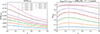 |
Fig. 1. Left: Variation in SNR values with α for different assumed values of SNRtot(2)∈[0.02, 0.10] (see plot annotation), with the vertical dotted line marking the standard value of α = 2 and the vertical dashed line marking the optimal value of α ≃ 1.2. The corresponding horizontal dotted and dashed lines mark the intersection with the red curve, having SNRtot(2) = 0.050. Right: Corresponding detection probabilities, pfinal, for νmax = 2000 μHz and T = 1 month. |
The right panel reveals a maximum in the curves at a value of α ≃ 1.2, marked with the dashed line. The standard value of α = 2 is seen to be sub-optimal. Other choices of νmax and T give essentially the same results, with some very small scatter in the optimal value for α. The largest gain appears to come at intermediate detection probabilities.
This behaviour is illustrated in Fig. 2, which shows how the change Δpfinal between α = 1.2 and 2.0 varies with νmax, pfinal (left column) and SNRtot(2) (right column). The top row shows results for T = 1 month, and the bottom row shows them for T = 6 months. The right panel reveals a well-constrained optimal region in νmax-SNR space. To the right of this region, the detection probability is already high, meaning little if any gain is to be had through changing α. The upper right half of the plot will, in practice, not contain real stars, because the maximum mode amplitudes and hence Ptot decrease strongly with increasing νmax. To the left of the optimal region, the SNR is so low that there is a negligible impact on the probability from changing α. The optimal region moves to higher SNR at lower νmax because  drops, meaning a higher SNR is required to give similar gains in probability. It is also shifted to higher SNR at lower T for the same reason. We note that increasing the false-alarm probability pfalse has the effect of moving the ridge in Δpfinal from Fig. 2 to lower SNRtot(2) values, and vice versa for a decreased pfalse.
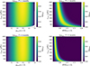 |
Fig. 2. Variation in the change Δpfinal between α = 1.2 and 2.0 with νmax, pfinal (left column) and SNRtot(2) (right column). The top row shows results for T = 1 month, and the bottom row shows them for T = 6 months. |
Figure 3 shows results of detectability predictions for a sample of bright stars observed by TESS (Ricker et al. 2015). Specifically, we adopted the V ≤ 6 stars from the TESS Luminaries Sample (Lund et al. 2025), which also includes the sample of bright evolved stars (their Fig. 1). Detectability predictions were made using the ATL3 tool of Hey et al. (2024)1, which implements the Chaplin et al. (2011) method, assuming a single sector of TESS observations (T ≃ 1 month), data with a cadence of 120 sec, a false-alarm probability of 5%, and input values of Teff, log g, and R from the Gaia DR3 gspphot (Gaia Collaboration 2023). Figure 3 shows the same structure as in the above calculations and plots, as well as the expected absence of stars in the upper right half of the νmax-SNR plot.
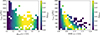 |
Fig. 3. Results for predictions using the bright TESS stars from the TESS Luminaries Sample (Lund et al. 2025), assuming a single sector of TESS observations (T ≃ 1 month), data with a cadence of 120 s, a false-alarm probability of 5%, and input values of Teff, log g, and R from the Gaia DR3 gspphot. |
For this specific sample, the predicted yield for pfinal ≥ 0.90 increased by ∼12% when we changed from α = 2 to 1.2, and by ∼5% for pfinal ≥ 0.99. This illustrates the benefits that accrue when considering the returns from a target ensemble. The improvement in the predicted yield strongly depends on the sample. For example, when a significantly longer observing duration is considered, many stars in a bright sample like the TESS one considered here would move to higher values of SNRtot(2) (to the right in Fig. 2), and the relative improvement in pfinal from changing α would decrease. Similarly, for a sample of dimmer stars, many would have very low SNRtot(2) values, and a longer observing duration T would be needed to see a significant relative change in pfinal from changing α.
4. Conclusion
We have presented a straightforward optimisation of the asteroseismic detection prediction recipe of Chaplin et al. (2011) by tuning the frequency range used for assessing the significance of excess power from solar-like oscillations. Instead of the range normally adopted, corresponding to twice the FWHM of the oscillation envelope (i.e. 2Γenv), we found that adopting a range of 1.2Γenv maximises the probability of detection.
Choices made over which scaling relations to adopt in the calculation of the mode and granulation parameters can clearly change the calculated probabilities, both positively and negatively. However, changing the adopted frequency range from 2Γenv to 1.2Γenv moves the predictions in one direction only, that is, to higher probabilities. Depending on the sample considered, this optimisation can have a substantial effect on the predicted detection yield. We therefore recommend the modification be implemented in target selection and detection prediction efforts for future missions suitable for asteroseismology, including the ESA PLATO Mission (Goupil et al. 2024), NASA’s Nancy Grace Roman Space Telescope (Weiss et al. 2025), and the proposed ESA High-precision AsteroseismologY of DeNse stellar fields (HAYDN) mission (Miglio et al. 2021). Furthermore, it is important to add that using our recommended range will also be beneficial for codes that analyse the data with the aim to detect solar-like oscillations, based on testing the significance of excess mode power (e.g. Appourchaux 2004; Lund et al. 2012; Bell et al. 2019; Viani et al. 2019; Nielsen et al. 2022), since its adoption will also optimise the probability of making robust detections.
Acknowledgments
MNL acknowledges support from the ESA PRODEX programme (PEA 4000142995). WJC acknowledges the support of the UK Space Agency. This research has made use of NASA’s Astrophysics Data System Bibliographic Services. We thank the referee for their helpful report.
References
- Appourchaux, T. 2004, A&A, 428, 1039 [NASA ADS] [CrossRef] [EDP Sciences] [Google Scholar]
- Appourchaux, T. 2014, in Asteroseismology, eds. P. L. Pallé, & C. Esteban, 123 [Google Scholar]
- Basu, S., & Chaplin, W. J. 2017, Asteroseismic Data Analysis: Foundations and Techniques (Princeton University Press) [Google Scholar]
- Bell, K. J., Hekker, S., & Kuszlewicz, J. S. 2019, MNRAS, 482, 616 [Google Scholar]
- Campante, T. L., Schofield, M., Kuszlewicz, J. S., et al. 2016, ApJ, 830, 138 [Google Scholar]
- Chaplin, W. J., & Miglio, A. 2013, ARA&A, 51, 353 [Google Scholar]
- Chaplin, W. J., Kjeldsen, H., Bedding, T. R., et al. 2011, ApJ, 732, 54 [CrossRef] [Google Scholar]
- Chaplin, W. J., Lund, M. N., Handberg, R., et al. 2015, PASP, 127, 1038 [NASA ADS] [CrossRef] [Google Scholar]
- Gaia Collaboration (Vallenari, A., et al.) 2023, A&A, 674, A1 [NASA ADS] [CrossRef] [EDP Sciences] [Google Scholar]
- García, R. A., & Ballot, J. 2019, Liv. Rev. Sol. Phys., 16, 4 [Google Scholar]
- Goupil, M. J., Catala, C., Samadi, R., et al. 2024, A&A, 683, A78 [NASA ADS] [CrossRef] [EDP Sciences] [Google Scholar]
- Hey, D., Huber, D., Ong, J., Stello, D., & Foreman-Mackey, D. 2024, ArXiv e-prints [arXiv:2403.02489] [Google Scholar]
- Kallinger, T., De Ridder, J., Hekker, S., et al. 2014, A&A, 570, A41 [NASA ADS] [CrossRef] [EDP Sciences] [Google Scholar]
- Larsen, J. R., Lundkvist, M. S., Nielsen, M. B., et al. 2026, A&A, accepted [arXiv:2602.08978] [Google Scholar]
- Lund, M. N. 2019, MNRAS, 489, 1072 [Google Scholar]
- Lund, M. N., Chaplin, W. J., & Kjeldsen, H. 2012, MNRAS, 427, 1784 [Google Scholar]
- Lund, M. N., Chaplin, W. J., Casagrande, L., et al. 2016, PASP, 128, 124204 [CrossRef] [Google Scholar]
- Lund, M. N., Basu, S., Bieryla, A., et al. 2024, A&A, 688, A13 [NASA ADS] [CrossRef] [EDP Sciences] [Google Scholar]
- Lund, M. N., Chontos, A., Grundahl, F., et al. 2025, A&A, 701, A285 [NASA ADS] [CrossRef] [EDP Sciences] [Google Scholar]
- Miglio, A., Girardi, L., Grundahl, F., et al. 2021, Exp. Astron., 51, 963 [NASA ADS] [CrossRef] [Google Scholar]
- Mosser, B., Belkacem, K., Goupil, M.-J., et al. 2010, A&A, 517, A22 [NASA ADS] [CrossRef] [EDP Sciences] [Google Scholar]
- Mosser, B., Elsworth, Y., Hekker, S., et al. 2012, A&A, 537, A30 [NASA ADS] [CrossRef] [EDP Sciences] [Google Scholar]
- Moya, A., Barceló Forteza, S., Bonfanti, A., et al. 2018, A&A, 620, A203 [NASA ADS] [CrossRef] [EDP Sciences] [Google Scholar]
- Nielsen, M. B., Hatt, E., Chaplin, W. J., Ball, W. H., & Davies, G. R. 2022, A&A, 663, A51 [NASA ADS] [CrossRef] [EDP Sciences] [Google Scholar]
- Ricker, G. R., Winn, J. N., Vanderspek, R., et al. 2015, J. Astron. Telesc. Instrum. Syst., 1, 014003 [Google Scholar]
- Schofield, M., Chaplin, W. J., Huber, D., et al. 2019, ApJS, 241, 12 [Google Scholar]
- Viani, L. S., Basu, S., Corsaro, E., Ball, W. H., & Chaplin, W. J. 2019, ApJ, 879, 33 [NASA ADS] [CrossRef] [Google Scholar]
- Weiss, T. J., Downing, N. J., Pinsonneault, M. H., et al. 2025, ApJ, 987, 181 [Google Scholar]
Updated with a TESS-specific bolometric correction for mode amplitudes (Lund 2019).
All Figures
|
Fig. 1. Left: Variation in SNR values with α for different assumed values of SNRtot(2)∈[0.02, 0.10] (see plot annotation), with the vertical dotted line marking the standard value of α = 2 and the vertical dashed line marking the optimal value of α ≃ 1.2. The corresponding horizontal dotted and dashed lines mark the intersection with the red curve, having SNRtot(2) = 0.050. Right: Corresponding detection probabilities, pfinal, for νmax = 2000 μHz and T = 1 month. |
| In the text | |
|
Fig. 2. Variation in the change Δpfinal between α = 1.2 and 2.0 with νmax, pfinal (left column) and SNRtot(2) (right column). The top row shows results for T = 1 month, and the bottom row shows them for T = 6 months. |
| In the text | |
|
Fig. 3. Results for predictions using the bright TESS stars from the TESS Luminaries Sample (Lund et al. 2025), assuming a single sector of TESS observations (T ≃ 1 month), data with a cadence of 120 s, a false-alarm probability of 5%, and input values of Teff, log g, and R from the Gaia DR3 gspphot. |
| In the text | |
Current usage metrics show cumulative count of Article Views (full-text article views including HTML views, PDF and ePub downloads, according to the available data) and Abstracts Views on Vision4Press platform.
Data correspond to usage on the plateform after 2015. The current usage metrics is available 48-96 hours after online publication and is updated daily on week days.
Initial download of the metrics may take a while.