| Issue |
A&A
Volume 708, April 2026
|
|
|---|---|---|
| Article Number | A266 | |
| Number of page(s) | 19 | |
| Section | Stellar structure and evolution | |
| DOI | https://doi.org/10.1051/0004-6361/202659096 | |
| Published online | 10 April 2026 | |
Long-term optical variability of high-mass X-ray binaries
III. Polarimetry
1
Institute of Astrophysics, Foundation for Research and Technology-Hellas, 71110 Heraklion, Greece
2
Physics Department, University of Crete, 71003 Heraklion, Greece
3
Max-Planck-Institut für Astronomie, Königstuhl 17, 69117 Heidelberg, Germany
★ Corresponding authors: This email address is being protected from spambots. You need JavaScript enabled to view it.
; This email address is being protected from spambots. You need JavaScript enabled to view it.
; This email address is being protected from spambots. You need JavaScript enabled to view it.
Received:
23
January
2026
Accepted:
26
February
2026
Abstract
Context. Systems known as Be/X-ray binaries form the most numerous group of high-mass X-ray binaries. Their long-term optical and infrared variability reflects the evolution of the circumstellar disk around the luminous companion. This variability manifests photometrically as an excess of flux that increases with wavelength and spectroscopically as line emission. The disk is also expected to generate linear polarization.
Aims. We present a systematic study of the optical long-term polarimetric variability of Be/X-ray binaries using data collected over ten years. Our aim is to characterize the polarimetric properties of these systems and to probe the structure of their circumstellar disks.
Methods. We monitored Be/X-ray binaries visible from the Northern Hemisphere with the RoboPol polarimeter. We performed a careful analysis of the interstellar polarization in the direction of the sources to estimate their intrinsic polarization. We computed Stokes parameters for linear polarization by aperture photometry and corrected them for instrumental polarization.
Results. Optical polarimetric variability is a common trait in Be/X-ray binaries. The variability can be attributed to the Be star’s circumstellar disk. Our polarization analysis confirms previous claims, based on spectroscopic data, that the circumstellar disks in BeXBs are, on average, smaller and more dense than those in Be stars in nonbinary systems. Our data also confirm the presence of highly distorted disks prior to giant X-ray outbursts, although this result is still limited by the lack of simultaneous, well-sampled observations during major X-ray outbursts.
Key words: binaries: general / stars: emission-line, Be / stars: neutron
© The Authors 2026
 Open Access article, published by EDP Sciences, under the terms of the Creative Commons Attribution License (https://creativecommons.org/licenses/by/4.0), which permits unrestricted use, distribution, and reproduction in any medium, provided the original work is properly cited.
This article is published in open access under the Subscribe to Open model. This email address is being protected from spambots. You need JavaScript enabled to view it. to support open access publication.
1. Introduction
Neutron star high-mass X-ray binaries (HMXBs) are accretion-powered binary systems in which the neutron star orbits an early-type (O or B) companion. The luminosity class of the optical companion subdivides HMXBs into Be/X-ray binaries (BeXBs), when the optical star is a dwarf, subgiant, or giant OBe star (luminosity class III, IV, or V), and supergiant X-ray binaries (SGXBs), when they contain an evolved star of luminosity class I–II. In SGXBs, the optical star emits a substantial stellar wind. A neutron star in a relatively close orbit captures a significant fraction of this wind, sufficient to power a bright X-ray source. In BeXBs, the donor is a Be star, that is, a rapidly rotating early-type B star with a gaseous equatorial disk (Reig 2011; Rivinius et al. 2013).
The disk forms when matter is ejected from the stellar photosphere with sufficient angular momentum. This type of disk is referred to as a decretion disk. The ultimate mechanism that lifts material onto the disk remains an open question, but the most likely candidates are a combination of fast rotation and nonradial pulsations (Baade 1992; Rivinius et al. 2013) or magnetic reconnection associated with localized magnetic fields generated by convection (Balona 2003; Balona & Ozuyar 2021). Martin et al. (2025) propose the presence of a boundary layer that connects a geometrically thick disk to a rotationally flattened star. The boundary layer provides the required torque and prevents the ejected material from falling back onto the star. In turn, the decretion disk exerts a torque on the star that slows the Be star’s rotation rate while still allowing decretion to continue.
The physical properties of the disk, such as density or physical extent, depend on whether the mass-outflow mechanism is active. Disks in Be stars form and dissipate, contributing to their long-term optical and IR variability. Because the disk is also the main reservoir of material available for accretion onto the compact object, its evolution is likewise reflected in the X-ray variability of Be/X-ray binaries. The largest-amplitude variations are typically observed on timescales of years, corresponding to the characteristic timescale for disk build-up and dissipation (Jones et al. 2008; Reig et al. 2016; Treiber et al. 2025).
Circumstellar disks in Be stars contribute to both the continuum and discrete (e.g., line) emission; this contribution appears in photometry, spectroscopy, and polarimetry:
-
Disk emission contributes to the overall brightness of the system and affects the photometric magnitudes and colors. The excess continuum radiation is small at short wavelengths (i.e., B band) and increases at longer wavelengths (i.e., H and K bands). The main disk contribution to the V band comes from a relatively small area near the star, whereas the emission area increases for longer wavelengths (Carciofi & Bjorkman 2006). As a result, the color indices increase , and the emission becomes redder as the disk develops.
-
The most prominent feature in the optical spectra of Be stars is the presence of emission lines, particularly those of the Balmer series. The hydrogen lines are optically thick and form in a large part of the disk by recombination. In particular, the Hα line stands out as the primary diagnostic of the disk state (Quirrenbach et al. 1997; Tycner et al. 2005; Grundstrom & Gies 2006). Large-amplitude variations in the strength and profile morphology are associated with structural changes of the circumstellar decretion disk (Reig et al. 2016).
-
The continuum polarization originates from Thomson scattering of initially unpolarized stellar radiation in the disk (Coyne & Kruszewski 1969; Serkowski 1970; Poeckert et al. 1979). Thomson scattering polarizes the radiation perpendicular to the scattering plane. The polarization degree provides information about the number of scatterers (i.e., the density). Consequently, changes in the polarization degree and position angle over time trace the evolution of the disk’s physical structure.
We have monitored the BeXBs visible from the Northern Hemisphere in the optical band with the 1.3 m telescope at Skinakas Observatory (SKO) since 1998, with the aim of investigating the evolution of their decretion disks. The monitoring consists of BVRI photometry and medium-resolution spectroscopy around the Hα line. The results of the photometric study appear in Reig & Fabregat (2015), while those of the spectroscopic observations appear in Reig et al. (2016). Since 2013, following the installation of the RoboPol polarimeter, we have also obtained optical polarimetric measurements of the same sources. The present work constitutes the third part of this series and reports the results of the polarimetric observations.
2. Data acquisition and analysis
2.1. Observations
The data were obtained from the SKO, located on the Ida mountain in central Crete, Greece, at an altitude of 1750 m. We obtained observations with the RoboPol polarimeter attached to the 1.3 m modified Ritchey-Chrétien telescope, an Andor DW436 CCD with an array of 2048 × 2048 13.5 μm pixel size (corresponding to 0.435 arcsec/pixel on the sky), providing a field of view of 13 square arcmin. The camera was cooled to −70°C, ensuring negligible dark current. The default monitoring setup uses a Johnson-Cousins R-band filter. However, observations at other band-passes are possible thanks to a five-slot filter wheel.
RoboPol is a four-channel imaging polarimeter that uses two Wollaston prisms and two nonrotating half-wave plates to produce simultaneous measurements of the Stokes Q and U parameters (Ramaprakash et al. 2019). RoboPol splits the incoming light into two light beams: one horizontal and the other vertical (see Fig. 1 in King et al. 2014). Thus, every point in the sky appears four times on the CCD. In each spot, we measured the photon counts using aperture photometry to calculate the normalized Stokes parameters q = Q/I and u = U/I of linear polarization, where I is the total intensity of the source. A mask in the telescope focal plane optimizes the instrument sensitivity. The absence of moving parts avoids possible errors caused by variations in sky conditions between measurements. Table 1 lists the targets; polarization measurements for each target appear as supplementary material (Appendix D) and are archived in the Zenodo repository1.
Target list and relevant information.
2.2. Instrumental polarization
When light passes through the various optical elements that constitute the optical system (telescope plus polarimeter), a low-level polarization is introduced into the observed radiation. This instrumental polarization appears as an additional polarization signal that requires correction. We accounted for this effect by measuring zero-polarized standard stars observed over multiple years. The average instrumental polarization in the R band is 0.4 ± 0.2%.
The data also require correction to align the rotation of the instrumental q − u plane with respect to the standard reference frame. We achieved this using highly polarized standards, monitored along with the unpolarized standard candidate sample. More details on these two corrections appear in Blinov et al. (2023).
2.3. Field stars
Stellar light travels through the interstellar medium (ISM) before observers detect it. The ISM introduces extra polarization from the nonsphericity of dust grains that align in a preferred direction due to the Galactic magnetic field (Lazarian et al. 2015; Tram & Hoang 2022). To correct for this extra polarization, we observed a number of field stars in the field of view of each target. We selected the field stars based on their proximity in absolute distance to the targets. Vector subtraction removes the interstellar component. The polarization measurements of the field stars appear as supplementary material (Appendix E) and are archived in the Zenodo repository.
2.4. Data analysis
We processed the data using the standard RoboPol pipeline described by King et al. (2014), with modifications presented by Blinov et al. (2021). The pipeline reads the raw images from the telescope and computes the Stokes parameters of the stars in the field of view by means of aperture photometry. It performs five tasks: (i) source identification, (ii) aperture photometry, (iii) calibration, (iv) polarimetry, and (v) relative photometry
The polarization degree (p) is defined as a function of the normalized Stokes parameters as
 (1)
(1)
with the corresponding uncertainty,
 (2)
(2)
where σq and σu are the uncertainties of the individual observations and include the contribution from the instrumental error uncertainty,
 (3)
(3)
and similarly for u. Unlike u and q, which are unbiased quantities and follow a normal distribution, the polarization degree is biased toward higher values at low signal-to-noise ratios and follows a Rician distribution. Various methods have been suggested for correcting this bias (Simmons & Stewart 1985; Vaillancourt 2006; Plaszczynski et al. 2014). In this work, we use the nondebiased values of the polarization degree, unless stated otherwise.
The electric vector polarization angle (EVPA) is defined as
 (4)
(4)
Because the EVPA does not follow a Gaussian distribution, we computed the uncertainty σθ numerically, by solving the following integral:
 (5)
(5)
Here, G(θ; θ0; p0) is the probability density followed by EPVA, (Naghizadeh-Khouei & Clarke 1993)
![Mathematical equation: $$ \begin{aligned} G(\theta ; \theta _0; p_0) = \frac{e^{-\frac{p_0^2}{2 \sigma ^2_p}}}{\sqrt{\pi }}\left\{ \frac{1}{\sqrt{\pi }}+\eta _0e^{\eta _0^2}[1+\mathrm {erf}(\eta _0)] \right\} , \end{aligned} $$](/articles/aa/full_html/2026/04/aa59096-26/aa59096-26-eq21.gif) (6)
(6)
where  , erf is the Gaussian error function, p0 and θ0 are the true values of p and EVPA, and σp is the uncertainty of p. We refer the reader to Blinov et al. (2023) for further details
3. Results
In this section, we present the results of our polarimetric analysis of the targets (Table 1). Our aim is to investigate whether BeXBs are intrinsically polarized and to study the connection between their long-term polarimetric variability and X-ray activity.
To determine whether a source is intrinsically polarized, we estimated and subtracted the ISM polarization from the observed polarization. various methods assess whether the measured polarization arises entirely from the ISM or whether some fraction is intrinsic to the source. These include multicolor polarimetry, variability analysis, empirical relationships between extinction and polarization degree in the Galaxy, and measurements of the polarization of field stars around the X-ray source.
-
The wavelength dependence of interstellar polarization differs from that of a Be star. Polarization in the ISM obeys the empirical relation given by Serkowski et al. (1975):
![Mathematical equation: $$ \begin{aligned} P(\lambda )/P_{\rm max}=\exp [-k \ln ^2(\lambda _{\rm max}/\lambda )] . \end{aligned} $$](/articles/aa/full_html/2026/04/aa59096-26/aa59096-26-eq23.gif) (7)
(7)The parameter k determines the width or sharpness of the curve. The wavelength at which the polarization is maximum, λmax, is directly related to the size of the dust grains (Coyne et al. 1974; Serkowski et al. 1975) and to the total-to-selective extinction, R = AV/E(B − V) (Whittet & van Breda 1978). The mean value of R = 3.05 corresponds to λmax = 0.545 μm (Whittet & van Breda 1978). A deviation from Serkowsky’s law indicates a certain amount of intrinsic polarization, although it can also result from multiple dust clouds with different properties along the line of sight (Mandarakas et al. 2025). In contrast, the polarization degree of unreddened Be stars peaks in the blue (λ ≈ 0.45 μm) and decreases with wavelength in the range 0.45–0.80 μm (Poeckert et al. 1979; McDavid 2001; Halonen et al. 2013; Haubois et al. 2014).
-
Because ISM polarization is expected to remain constant for a given direction, if a source’s polarization degree is variable, then a fraction of it is intrinsic to the source. However, quantifying the actual amount of intrinsic polarization through variability analysis is not possible unless the system allows for the definition of a zero-level intrinsic polarization. Be stars provide such a method. As mentioned above, polarization in Be stars arises from electron scattering in the circumstellar disk. If the disk is absent, all contributions to the polarization parameters should come from the ISM. We discuss disk-loss events in Sect. 4.1.1.
-
As dust accumulates along a line of sight with increasing distance, the degree of polarization associated with a star also depends on its distance, or equivalently, on extinction. Several authors (Hiltner 1956; Serkowski et al. 1975; Jones 1989; Reiz & Franco 1998; Fosalba et al. 2002; Ignace et al. 2025) have studied the relationship between polarization and extinction. These studies confirm that the ISM polarization fraction increases as the extinction (or distance) increases, albeit with a large scatter. However, these studies are limited to relatively close stars with E(B − V)≲1 mag. The alignment and uniformity of the magnetic field are expected to disappear as the line of sight crosses increasing interstellar dust clouds. The resulting polarization of the most distant objects becomes a function of the cloud parameters (orientation and strength of their magnetic fields). Thus, more distant objects are expected to suffer depolarization. For example, Fosalba et al. (2002) found that the polarization degree as a function of distance shows a maximum for stars at 2 − 4 kpc and then decreases slightly for more distant objects up to 6 kpc. Similarly, using ∼28 000 stars from the catalog of Panopoulou et al. (2025), Ignace et al. (2025) report that the median polarization fraction increases up to ∼1 kpc and then flattens for larger distances.
-
The most reliable method for estimating ISM polarization is to observe a sample of field stars located at distances similar to that of the source. The measured Stokes u and q of the field stars are then subtracted from the measured polarization of the targets.
In the following sections, we address each of these methods. We show the results for a selected number of targets, chosen as representative cases. Results for all the sources are presented in the Appendices.
3.1. Wavelength dependence
We conducted polarimetric monitoring of the Galactic BeXBs visible from the northern hemisphere in the R band. We also observed several sources in the B, V, and I bands. This multicolor photometry enables, in principle, an investigation of the wavelength dependence of the polarization. In practice, however, due to the scarcity of the data (only four data points) and the limited wavelength range, the analysis did not yield conclusive results. Therefore, we did not pursue this method.
3.2. Measuring variability using the variability diagram
In this section, we study the long-term polarimetric variability. Since ISM polarization is expected to remain constant for a given direction and distance in the sky, and to avoid introducing additional uncertainty inherent to the field stars, we performed the analysis on the data corrected for instrumental polarization only, without subtracting the ISM contribution.
To study variability, we followed the methodology of Blinov et al. (2023), which is based on a statistical test using the cumulative distribution function (CDF) of the polarization data (Clarke & Naghizadeh-Khouei 1994; Bastien et al. 2007). The method compares the theoretical CDF with the empirical distribution function (EDF) using a two-sided Kolmogorov-Smirnov (KS) test. If the p-value of the KS test exceeds a threshold (e.g., p = 0.0027 corresponds to a 3σ confidence level), we consider the star to be nonvariable.
The theoretical CDF for a nonpolarized source normalized by its errors,  , is given by
 (8)
(8)
and the EDF by
 (9)
(9)
where q and u are the Stokes parameters. For a polarized star, Eq. (8) does not apply. To avoid this situation, we subtracted the weighted mean values,  and
and  , to make the source appear unpolarized: (Clarke & Naghizadeh-Khouei 1994; Blinov et al. 2023)
 (10)
(10)
We present plots showing the long-term evolution of the polarization degree (PD) and the EVPA for all targets in Appendix A. Figure 1 illustrates the BeXB RXJ0146.9+6121. The left panels show the evolution of the Stokes parameters u and q, the PD and the EVPA. The upper-right panel displays the q − u plane. In this panel, the black circles correspond to the weighted mean of the source computed yearly, while the red cross represents the weighted mean of the field stars used later to derive the intrinsic polarization. The bottom-right panel compares the theoretical CDF (blue line) and the empirical EDFs for the entire set of observations (i.e., black circles in the evolution plots, black line) and the seasonal weighted mean (red circles, red line). Rather than assuming a given threshold to assess source variability, we provide the p-value derived from the KS test2. Table 2 lists the normal mean and standard deviation of the entire dataset for each BeXB. Columns 10 and 11 show the computed p-value of the KS test. We find that 18 of the 22 sources vary at > 3σ level on timescales of years.
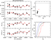 |
Fig. 1. Left: Evolution of the Stokes parameters, polarization degree and angle. Top right: q − u plane. Weighted mean of the source observations (black circles), calculated yearly, and of the field stars (red cross). Bottom right: Empirical distribution function (EDF) of measured polarization using all data points (black line) or the weighted averaged points (red line) compared with expected cumulative distribution function (CDF) of polarization measurements (blue line). The data shown correspond to the BeXB RX J0146.9+6121. |
3.3. Extinction
The relationship between polarization degree and extinction shows a large dispersion. For many years, the theoretical upper limit for the optimal alignment efficiency of dust grains with external magnetic fields was P(%) = 9E(B − V) (Serkowski et al. 1975; Reiz & Franco 1998). However, cases in which the observed starlight polarization exceeds the classical upper limit and reaches PV/E(B − V) = 14% are reported (Panopoulou et al. 2019; Bartlett & Kobulnicky 2025). Nevertheless, the observed mean correlation between polarization degree and extinction for data averaged in extinction bins is much smaller and deviates slightly from the simple linear correlation, P(%) = 3.5E(B − V)0.8 (Fosalba et al. 2002).
Figure 2 shows the extinction curves for IGR J06074+2205 and XTE J1946+274 as examples of a well-behaved case, in which the PD increases with distance, and a more complex case associated with a larger and more uncertain distance, respectively. We marked the locations of the field stars and the source according to their distances. We took the extinction data from the dust maps by Green et al. (2019). These figures provide a simple way to estimate the number of molecular clouds to the source, although the distance range over which the data are reliable is limited because of the insufficient number of stars with reddening estimates. This range varies from source to source and is indicated by a vertical dashed line in the figures.
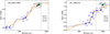 |
Fig. 2. Two representative examples of extinction as a function of distance (data from Green et al. 2019). Data points mark the assumed locations of the stars on the extinction curve, based on their distances; they do not imply extinction values. Distances are from Bailer-Jones et al. (2021). The turquoise circle represents the BeXB, the black circles show the field stars used for the ISM correction, and the blue circles correspond to other field stars. We also indicate the polarization degree (PD) of the field stars. The vertical dashed line marks the region of uncertain extinction. |
Polarization statistics.
Appendix B shows the individual extinction curves for each source.
3.4. Field stars
The most common method to account for ISM polarization uses field stars. We observed several stars within ∼7 arcmin of each target at comparable distances. Distances were taken from Gaia DR3 (Bailer-Jones et al. 2021). The polarization measurements of the field stars are given in Appendix E (Supplementary material in the Zenodo repository3). The weighted means of the Stokes parameters u and q also appear in the variability plots (Fig. 1). However, this method carries uncertainty because the dust distribution (e.g., orientation of the dust grains) and the number of intervening molecular clouds along the line of sight may be complex (see the right panel in Fig. 2). In addition, some field stars may exhibit nonzero intrinsic polarization, contrary to the assumption of this method that they are intrinsically unpolarized. It is therefore advisable to employ multiple field stars. Owing to this uncertainty, the results of the observations given in the appendix correspond to the measured polarization values, without correction for ISM contribution. This approach allows readers to apply their own selection of field stars for ISM subtraction. Appendix C presents sky charts that identify the target and field stars.
4. Discussion
An objective of this work is to study the evolution of decretion disks in BeXBs through polarization observations. Changes in the polarization angle and polarization degree trace evolutionary changes in the geometry and physical extent of the disk. Electron scattering of unpolarized light generates polarized radiation perpendicular to the scattering plane, which in Be stars coincides with the decretion disk. This occurs because multiple scattering occurs predominantly in the optically thicker equatorial regions. This biases the orientation of the scattering planes of multiply scattered photons toward the equatorial plane (Wood et al. 1996). Therefore, variability in the polarization angle may reveal the presence of warped disks (Reig & Blinov 2018). Likewise, because the polarization degree provides information about the number of scatterers, it can be linked to the disk density.
4.1. Long-term variability
Section 3.2 shows that most BeXBs exhibit polarimetric variability on timescales of years. Only three systems, SAX J2239.3+6116, IGR J01363+6610, and IGR J0158+6713, display stable long-term polarization (< 2σ). However, even in these cases, the standard deviation computed over the entire dataset (Table 2) is significantly greater than the instrument accuracy, which is estimated to be better than 0.015% based on measurements of standard stars. These timescales correspond to the viscous timescale of Be star’s disk evolution. Two natural consequences of the long-term variability associated with disk evolution are disk loss and the occurrence of X-ray outbursts.
4.1.1. Disk-loss episodes
Circumstellar disks in Be stars, and therefore also in BeXBs, are not permanent features. They form, grow, and dissipate on timescales of years. Disk-loss episodes are of paramount importance because they enable the separation of intrinsic polarization from that due to the ISM. In Be stars, linear polarization originates in the circumstellar disk. Thus, in the absence of the disk, the measured polarization must be entirely interstellar in origin. The Hα line is the most reliable indicator of disk dissipation: it changes from emission to a pure absorption profile once the disk has been lost. Consequently, its equivalent width (EW) serves as a robust proxy for the presence or absence of the disk. By convention, EW is negative for emission lines and positive for absorption lines.
Table 3 lists the maximum and minimum EW(Hα) values for the studied targets during the period 2013–2024, which corresponds to our polarimetric campaigns. The spectroscopic data were obtained with the 1.3 m telescope at SKO and are part of a long-term monitoring project4. Three BeXBs underwent disk-loss episodes: IGR J06074+2205, SAX J2103.5+4545, and IGR J21343+4738, while five others showed evidence of highly debilitated disks: 4U 0115+63, RX J0440.9+4431, MXB 0656–072, GRO J2058+42, and SAX J2239.3+6116. Table 4 compares the PD during low optical states, including disk-loss events, with the PD derived from field-star analysis. In general, the agreement is good, especially in cases where the absence of the disk is most evident. For sources with EW(Hα) > 0, it is expected that a small residual disk remains. For RX J0440.9+4431, the suitability of field stars may be questioned because they are located at a greater distance than the target.
Minimum and maximum Hα equivalent widths.
Polarization degree during low-optical states (including disk-loss events) and from field-star analysis.
4.1.2. Giant X-ray outbursts
X-ray outbursts in Be/X-ray binaries originate when mass from the Be star’s circumstellar disk transfers to the neutron star. However, the exact transfer mechanism remains unclear. The disks in Be/X-ray binaries are often truncated due to the gravitational effects of the neutron star (Reig et al. 1997a; Negueruela & Okazaki 2001; Okazaki & Negueruela 2001; Reig et al. 2016). This truncation raises the question of how substantial matter transfers to the neutron star to trigger the X-ray outbursts. If the disk is truncated, substantial accretion is only feasible if the disk becomes asymmetric and dense enough to exceed the truncation radius. Current theory suggests that giant outbursts occur when the neutron star captures a significant amount of gas from a warped, highly misaligned, and eccentric Be disk (Martin et al. 2011; Okazaki et al. 2013; Martin et al. 2014). Models indicate that these highly distorted disks enhance mass accretion when the neutron star passes through the warped region. This interaction increases the density and volume of gas available for accretion onto the neutron star, thereby triggering intense X-ray emission.
Observational evidence for warped disks comes from spectral lines. Low inclination systems produce single peak profiles, intermediate inclination systems produce double-peak profiles, and high-inclination systems generate shell profiles (Rivinius et al. 2013). Therefore, if a single source shows all these profiles, and since the spin axis of the Be star is not expected to change on timescales of days, the appearance of different profiles in the same star implies that the disk axis changes direction. In other words, the source hosts a warped precessing disk. Changes in the emission line profile in Be and BeXBs have been interpreted as observational evidence for misaligned disks that become warped in their outer parts (Hummel 1998; Negueruela et al. 2001; Reig et al. 2007; Moritani et al. 2011, 2013).
Further evidence for warped disks should come from the polarization angle, because Thompson scattering polarizes light perpendicular to the scattering plane. Therefore, if the orientation of the disk changes, the polarization angle should also change. Table 5 lists the sources that exhibited a giant (type II) outburst during the period covered by the polarimetric observations. We computed data from the Swift/BAT light curves using the average conversion factors listed in the table footnote. We searched for changes in the polarization parameters during type II outbursts. Figure 3 shows the polarization degree and angle during type II outbursts for the sources that underwent type II outbursts during the observations. The vertical dashed lines mark the peak of the X-ray outburst. The lack of data during many outbursts prevents us from providing strong evidence for warped precessing disks. Nevertheless, we identified promising cases. In addition to 4U 0115+63, previously reported by Reig & Blinov (2018), KS 1947+300, EXO 2030+375 and Swift J0243.6+6124 showed changes in EVPA that coincide with the X-ray outburst.
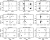 |
Fig. 3. Polarization degree and angle near a major (type II) X-ray outburst. The vertical dashed lines indicate the peak of the X-ray outburst. |
Type II outbursts during the observation period.
The outer parts of the disk are expected to be the most affected by warping effects (Martin & Franchini 2021), while the inner regions, where most of the polarization is produced, would be less affected. Linear polarization signatures arise primarily in the inner parts of the disk, where the density of scatterers is highest (Carciofi 2011; Halonen & Jones 2013b). This may explain the relatively small observed variation in EVPA (≲10°), which would be associated with the precession angle.
Fig. 3 shows that the distorted disk appears to precede the X-ray event. Except for Swift J0243.6+6124, for which no data were available prior to the outburst, the polarization parameters began to vary before the outburst onset in the other three cases. Thus, the presence of a distorted disk seems to be a prerequisite to trigger an X-ray outburst, consistent with theoretical predictions (Martin et al. 2011; Okazaki et al. 2013; Martin et al. 2014).
4.2. Short-term variability
In addition to long-term variations, Fig. 1 (and Appendix A) shows significant scatter, with polarization parameters varying by 10–30% on timescales of a few weeks to months. This behavior has been seen in isolated Be stars (Vince et al. 1995; Draper et al. 2014). The origin of this generally nonperiodic variability is unclear and likely stems from a diversity of phenomena that alter the distribution and density of the light scattering material in the disk. Longer-term phenomena (months) associated with these apparent stochastic jumps in polarization may include a rotating or precessing tilted disk (Marr et al. 2018) or one-armed density waves (Halonen & Jones 2013b; Draper et al. 2014); on much shorter timescales (≲1 day), polarimetric variability may be associated with mass ejection episodes from the Be star into the disk and from stochastic changes in the mass decretion rate (Carciofi et al. 2007; Wisniewski et al. 2010; Carciofi et al. 2025). On intermediate timescales (weeks), orbital modulation may also contribute to the scatter (Kravtsov et al. 2020).
4.3. Comparison with Be stars
The circumstellar disks in BeXBs are, on average, smaller and denser than those of Be stars in nonbinary systems. Evidence for this result comes from both observations (Reig et al. 1997a, 2000, 2016; Zamanov et al. 2001) and theory (Okazaki et al. 2002; Panoglou et al. 2016; Cyr et al. 2017). Disk truncation explains this phenomenon, resulting from the interaction between the disk and the neutron star. The closer the two components of the binary, the stronger the tidal torque exerted by the neutron star on the disk. Systems with short orbital periods (Porb ≲ 50 d) exhibit faster variability (i.e., rapid, irregular changes) than systems with longer orbital periods (see Fig. 1 in Reig et al. 2016). In narrow-orbit systems, the disk is exposed to larger torques from the neutron star, preventing it from reaching a stable configuration for a long period of time. Another example is the correlation between the maximum EW(Hα) and the orbital period in BeXBs (Reig et al. 1997a; Reig 2011). Because EW(Hα) provides a measure of the extent of the disk (Tycner et al. 2005; Grundstrom & Gies 2006), the correlation implies that only wider-orbit systems are able to develop stable and larger disks.
We investigated whether the polarization data agree with these results. For this analysis to be meaningful, the intrinsic polarization must be used. We corrected the measured polarization for the contribution of the ISM, as described in Sect. 3.4. The right panel of Fig. 4 shows the maximum intrinsic polarization degree, P*, as a function of the orbital period, Porb. There is a trend for larger intrinsic PD for wider-orbit systems in BeXBs. Excluding the outlier EXO 2030+375 and the Be/γ-ray binary RX J0240.4+6112/LS I +613035, the correlation is significant, with a correlation coefficient r = 0.66 and a probability that the null hypothesis (that the two variables are uncorrelated) is true of p-value = 0.015. Several factors could contribute to the dispersion in this plot: (i) uncertainty in the ISM polarization estimation, (ii) the dependence of the polarization fraction on inclination angle (Wood et al. 1996; Halonen et al. 2013), and/or (iii) the fact that polarization occurs closer to the Be star than the formation region of the Hα line (Carciofi 2011). In this respect, EW(Hα) provides a better proxy for the extent of the disk, and tidal interaction effects with the neutron star are more apparent. The intrinsic polarization fraction and angle strongly depend on the polarization of the field stars. However, the fact that there is no clear trend (r = 0.26, p-value = 0.34) between the maximum intrinsic polarization and the distance (left panel in Fig. 4) indicates adequate field star selection overall. Nevertheless, a bad representation of the ISM for some individual systems cannot be ruled out. The case of EXO 2030+375 is unique. It exhibits the highest polarization degree ever measured in either a Be star or a BeXB, well above the typical values observed in these systems (see discussion below). One possible explanation for this apparent extreme behavior is the high and spatially complex extinction toward the source. Figure C.1 and Appendix E (supplementary material in the Zenodo repository6) show a substantial variation in degree of polarization in the vicinity of the X-ray source. For instance, we observe clear differences when comparing the spatial locations and polarization degrees of the field stars gfs1 and gfs3, as well as gfs9 and gfs10. In this scenario, the high polarization observed in EXO 2030+375 results from an inaccurate correction for ISM polarization rather than from an intrinsic origin. Reig et al. (2014) proposed an alternative physical explanation for the unusually large PD in EXO 2030+375: they suggested that the high polarization arises from the alignment of nonspherical ferromagnetic grains in the Be-star disk under the influence of the neutron star’s strong magnetic field.
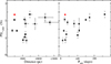 |
Fig. 4. Maximum intrinsic polarization degree as a function of distance (left) and orbital period (right), excluding the outlier EXO 2030+375. The red point corresponds to the Be/γ-ray binary RX J0240.4+6112/LS I +61303. |
The scatter is larger among the short-period systems (Porb ≲ 50 d). This trend also appears in the Hα equivalent width versus orbital period diagram (Reig et al. 2016) and in the X-ray band (Reig 2007). A simple explanation is that wider orbit systems can develop stable disks over longer time periods. In contrast, systems with short orbital periods experience stronger and more frequent tidal truncation from the neutron star, preventing the disk from reaching a stable configuration on shorter timescales.
Yudin (2001) performed a statistical analysis of the intrinsic polarization of 497 isolated Be stars covering the entire spectral range. The study found that, for the early-type group (B0-B3), which is the relevant group for comparison with BeXBs, values showed larger scatter, but on average, Be stars in this spectral range exhibited higher polarization. The maximum intrinsic polarization values for B0-B3 stars are PD*(%)≲2%. In the Yudin (2001) sample, only five stars exhibited polarization degrees above 2% (all in the B0-B2 spectral range). The average intrinsic polarization for different spectral subtypes in the Yudin sample was 0.84 ± 0.48% for O-B1.5 and 0.75 ± 0.48% for B2-B2.5.
About half of our BeXB sample displays an intrinsic maximum polarization degree above 2%. Figure 5 shows the normalized histogram of the maximum measured intrinsic PD in BeXBs compared to classical Be stars of similar spectral type range (data from Yudin 2001). Since the polarization degree reflects the number of scatterers, models predict that polarization increases with density, as the number of electrons available for Thomson scattering increases (Halonen & Jones 2013a). Our findings thus support the idea that disks in BeXBs are denser than in isolated Be stars.
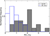 |
Fig. 5. Normalized histogram of the maximum intrinsic polarization (corrected for the ISM) for our BeXB sample, excluding the outlier EXO 2030+375, compared with the polarization distribution of classical Be stars of similar spectral type (data from Yudin 2001). The Y axis is computed so that the total area under the histogram equals 1. |
5. Conclusions
We performed a systematic study of the polarization properties of BeXBs visible from the Northern Hemisphere to characterized their long-term optical variability and to probe the dynamics and structure of their circumstellar disks. Our findings confirm that BeXBs are intrinsically variable in polarization, with changes in polarization degree and angle directly tracing the evolution of the disk size and geometry. A key result of this work is the confirmation that circumstellar disks in BeXBs are, on average, smaller and significantly denser than those in isolated Be stars. This finding is evidenced by the higher intrinsic polarization values observed in our sample, with approximately half of the targets exceeding the typical maximum polarization of isolated Be stars. This finding strongly supports theoretical models of disk truncation, where the gravitational influence of the neutron star tidally truncates and confines the Be star’s disk. We also find evidence linking giant X-ray outbursts to the presence of warped and precessing disks, where changes in the polarization angle, indicating a distorted disk, appear to be a necessary precursor to those high-energy events.
In conclusion, this study highlights the importance of polarimetry, together with spectroscopy and photometry, as diagnostic tools for investigating the physical mechanisms that govern the behavior of these complex binary systems.
Data availability
The polarization measurements, including q, u, PD, and EVPA, along with their corresponding uncertainties, are available in the Zenodo repository: https://doi.org/10.5281/zenodo.18346735
Acknowledgments
Skinakas Observatory is a collaborative project of the University of Crete and the Foundation for Research and Technology-Hellas. D.B. acknowledges support from the European Research Council (ERC) under the Horizon ERC Grants 2021 programme under grant agreement No. 101040021. This work made use of NASA’s Astrophysics Data System Bibliographic Services and of the SIMBAD database, operated at the CDS, Strasbourg, France. This work has made use of data from the European Space Agency (ESA) mission Gaia (https://www.cosmos.esa.int/gaia).
References
- Aragona, C., McSwain, M. V., Grundstrom, E. D., et al. 2009, ApJ, 698, 514 [Google Scholar]
- Baade, D. 1992, in The Atmospheres of Early-Type Stars, eds. U. Heber, & C. S. Jeffery, 401, 143 [Google Scholar]
- Bailer-Jones, C. A. L., Rybizki, J., Fouesneau, M., Demleitner, M., & Andrae, R. 2021, AJ, 161, 147 [Google Scholar]
- Balona, L. A. 2003, Ap&SS, 284, 121 [NASA ADS] [CrossRef] [Google Scholar]
- Balona, L. A., & Ozuyar, D. 2021, ApJ, 921, 5 [NASA ADS] [CrossRef] [Google Scholar]
- Bartlett, J. A., & Kobulnicky, H. A. 2025, AJ, 170, 265 [Google Scholar]
- Bastien, P., Vernet, E., Drissen, L., et al. 2007, ASP Conf. Ser., 364, 529 [Google Scholar]
- Baykal, A., Stark, M. J., & Swank, J. 2000, ApJ, 544, L129 [NASA ADS] [CrossRef] [Google Scholar]
- Blay, P., Negueruela, I., Reig, P., et al. 2006, A&A, 446, 1095 [NASA ADS] [CrossRef] [EDP Sciences] [Google Scholar]
- Blinov, D., Kiehlmann, S., Pavlidou, V., et al. 2021, MNRAS, 501, 3715 [NASA ADS] [CrossRef] [Google Scholar]
- Blinov, D., Maharana, S., Bouzelou, F., et al. 2023, A&A, 677, A144 [NASA ADS] [CrossRef] [EDP Sciences] [Google Scholar]
- Bonnet-Bidaud, J. M., & Mouchet, M. 1998, A&A, 332, L9 [NASA ADS] [Google Scholar]
- Carciofi, A. C. 2011, IAU Symp., 272, 325 [NASA ADS] [Google Scholar]
- Carciofi, A. C., & Bjorkman, J. E. 2006, ApJ, 639, 1081 [Google Scholar]
- Carciofi, A. C., Magalhães, A. M., Leister, N. V., Bjorkman, J. E., & Levenhagen, R. S. 2007, ApJ, 671, L49 [NASA ADS] [CrossRef] [Google Scholar]
- Carciofi, A. C., Bolzan, G. P. P., Querido, P. R., et al. 2025, Galaxies, 13, 77 [Google Scholar]
- Chhotaray, B., Naik, S., Jaisawal, G. K., & Ahuja, G. 2024, MNRAS, 534, 2830 [Google Scholar]
- Clarke, D., & Naghizadeh-Khouei, J. 1994, AJ, 108, 687 [NASA ADS] [CrossRef] [Google Scholar]
- Corbet, R. H. D., Markwardt, C. B., & Tueller, J. 2007, ApJ, 655, 458 [NASA ADS] [CrossRef] [Google Scholar]
- Coyne, G. V., & Kruszewski, A. 1969, AJ, 74, 528 [Google Scholar]
- Coyne, G. V., Gehrels, T., & Serkowski, K. 1974, AJ, 79, 581 [Google Scholar]
- Cyr, I. H., Jones, C. E., Panoglou, D., Carciofi, A. C., & Okazaki, A. T. 2017, MNRAS, 471, 596 [NASA ADS] [CrossRef] [Google Scholar]
- Doroshenko, V., Tsygankov, S., & Santangelo, A. 2016, A&A, 589, A72 [NASA ADS] [CrossRef] [EDP Sciences] [Google Scholar]
- Draper, Z. H., Wisniewski, J. P., Bjorkman, K. S., et al. 2014, ApJ, 786, 120 [NASA ADS] [CrossRef] [Google Scholar]
- Dubus, G. 2013, A&ARv, 21, 64 [Google Scholar]
- Esposito, P., Israel, G. L., Sidoli, L., et al. 2013, MNRAS, 433, 2028 [Google Scholar]
- Ferrigno, C., Farinelli, R., Bozzo, E., et al. 2013, A&A, 553, A103 [NASA ADS] [CrossRef] [EDP Sciences] [Google Scholar]
- Fosalba, P., Lazarian, A., Prunet, S., & Tauber, J. A. 2002, ApJ, 564, 762 [NASA ADS] [CrossRef] [Google Scholar]
- Galloway, D. K., Morgan, E. H., & Levine, A. M. 2004, ApJ, 613, 1164 [NASA ADS] [CrossRef] [Google Scholar]
- Green, G. M., Schlafly, E., Zucker, C., Speagle, J. S., & Finkbeiner, D. 2019, ApJ, 887, 93 [NASA ADS] [CrossRef] [Google Scholar]
- Grundstrom, E. D., & Gies, D. R. 2006, ApJ, 651, L53 [NASA ADS] [CrossRef] [Google Scholar]
- Grundstrom, E. D., Boyajian, T. S., Finch, C., et al. 2007, ApJ, 660, 1398 [NASA ADS] [CrossRef] [Google Scholar]
- Haigh, N. J., Coe, M. J., & Fabregat, J. 2004, MNRAS, 350, 1457 [NASA ADS] [CrossRef] [Google Scholar]
- Halonen, R. J., & Jones, C. E. 2013a, ApJ, 765, 17 [Google Scholar]
- Halonen, R. J., & Jones, C. E. 2013b, ApJS, 208, 3 [Google Scholar]
- Halonen, R. J., Mackay, F. E., & Jones, C. E. 2013, ApJS, 204, 11 [NASA ADS] [CrossRef] [Google Scholar]
- Haubois, X., Mota, B. C., Carciofi, A. C., et al. 2014, ApJ, 785, 12 [NASA ADS] [CrossRef] [Google Scholar]
- Hiltner, W. A. 1956, ApJS, 2, 389 [NASA ADS] [CrossRef] [Google Scholar]
- Hummel, W. 1998, A&A, 330, 243 [NASA ADS] [Google Scholar]
- Ignace, R., Fullard, A. G., Panopoulou, G. V., et al. 2025, Ap&SS, 370, 57 [Google Scholar]
- in’t Zand, J. J. M., Swank, J., Corbet, R. H. D., & Markwardt, C. B. 2001, A&A, 380, L26 [CrossRef] [EDP Sciences] [Google Scholar]
- Jones, T. J. 1989, ApJ, 346, 728 [Google Scholar]
- Jones, C. E., Sigut, T. A. A., & Porter, J. M. 2008, MNRAS, 386, 1922 [Google Scholar]
- Kaur, R., Paul, B., Kumar, B., & Sagar, R. 2008, MNRAS, 386, 2253 [NASA ADS] [CrossRef] [Google Scholar]
- King, O. G., Blinov, D., Ramaprakash, A. N., et al. 2014, MNRAS, 442, 1706 [NASA ADS] [CrossRef] [Google Scholar]
- Kızıloǧlu, U., Kızıloǧlu, N., Baykal, A., Yerli, S. K., & Özbey, M. 2007, A&A, 470, 1023 [NASA ADS] [CrossRef] [EDP Sciences] [Google Scholar]
- Kravtsov, V., Berdyugin, A. V., Piirola, V., et al. 2020, A&A, 643, A170 [NASA ADS] [CrossRef] [EDP Sciences] [Google Scholar]
- Lazarian, A., Andersson, B.-G., & Hoang, T. 2015, in Polarimetry of Stars and Planetary Systems, eds. L. Kolokolova, J. Hough, & A.-C. Levasseur-Regourd, 81 [Google Scholar]
- Liu, W., Reig, P., Yan, J., et al. 2025, ApJ, 985, 162 [Google Scholar]
- Mandarakas, N., Tassis, K., & Skalidis, R. 2025, A&A, 698, A168 [NASA ADS] [CrossRef] [EDP Sciences] [Google Scholar]
- Marcu-Cheatham, D. M., Pottschmidt, K., Kühnel, M., et al. 2015, ApJ, 815, 44 [Google Scholar]
- Marr, K. C., Jones, C. E., & Halonen, R. J. 2018, ApJ, 852, 103 [NASA ADS] [CrossRef] [Google Scholar]
- Martin, R. G., & Franchini, A. 2021, ApJ, 922, L37 [NASA ADS] [CrossRef] [Google Scholar]
- Martin, R. G., Pringle, J. E., Tout, C. A., & Lubow, S. H. 2011, MNRAS, 416, 2827 [NASA ADS] [CrossRef] [Google Scholar]
- Martin, R. G., Nixon, C., Armitage, P. J., Lubow, S. H., & Price, D. J. 2014, ApJ, 790, L34 [Google Scholar]
- Martin, R. G., Lubow, S. H., Vallet, D., et al. 2025, MNRAS, 539, L31 [Google Scholar]
- McDavid, D. 2001, ApJ, 553, 1027 [Google Scholar]
- Moritani, Y., Nogami, D., Okazaki, A. T., et al. 2011, PASJ, 63, 25 [Google Scholar]
- Moritani, Y., Nogami, D., Okazaki, A. T., et al. 2013, PASJ, 65, 83 [NASA ADS] [Google Scholar]
- Naghizadeh-Khouei, J., & Clarke, D. 1993, A&A, 274, 968 [NASA ADS] [Google Scholar]
- Negueruela, I., & Okazaki, A. T. 2001, A&A, 369, 108 [NASA ADS] [CrossRef] [EDP Sciences] [Google Scholar]
- Negueruela, I., Roche, P., Fabregat, J., & Coe, M. J. 1999, MNRAS, 307, 695 [NASA ADS] [CrossRef] [Google Scholar]
- Negueruela, I., Okazaki, A. T., Fabregat, J., et al. 2001, A&A, 369, 117 [NASA ADS] [CrossRef] [EDP Sciences] [Google Scholar]
- Nespoli, E., Reig, P., & Zezas, A. 2012, A&A, 547, A103 [NASA ADS] [CrossRef] [EDP Sciences] [Google Scholar]
- Okazaki, A. T., & Negueruela, I. 2001, A&A, 377, 161 [NASA ADS] [CrossRef] [EDP Sciences] [Google Scholar]
- Okazaki, A. T., Bate, M. R., Ogilvie, G. I., & Pringle, J. E. 2002, MNRAS, 337, 967 [NASA ADS] [CrossRef] [Google Scholar]
- Okazaki, A. T., Hayasaki, K., & Moritani, Y. 2013, PASJ, 65, 41 [NASA ADS] [Google Scholar]
- Panoglou, D., Carciofi, A. C., Vieira, R. G., et al. 2016, MNRAS, 461, 2616 [Google Scholar]
- Panopoulou, G. V., Hensley, B. S., Skalidis, R., Blinov, D., & Tassis, K. 2019, A&A, 624, L8 [NASA ADS] [CrossRef] [EDP Sciences] [Google Scholar]
- Panopoulou, G. V., Markopoulioti, L., Bouzelou, F., et al. 2025, ApJS, 276, 15 [NASA ADS] [CrossRef] [Google Scholar]
- Parmar, A. N., White, N. E., Stella, L., Izzo, C., & Ferri, P. 1989, ApJ, 338, 359 [NASA ADS] [CrossRef] [Google Scholar]
- Plaszczynski, S., Montier, L., Levrier, F., & Tristram, M. 2014, MNRAS, 439, 4048 [NASA ADS] [CrossRef] [Google Scholar]
- Poeckert, R., Bastien, P., & Landstreet, J. D. 1979, AJ, 84, 812 [NASA ADS] [CrossRef] [Google Scholar]
- Quirrenbach, A., Bjorkman, K. S., Bjorkman, J. E., et al. 1997, ApJ, 479, 477 [NASA ADS] [CrossRef] [Google Scholar]
- Raichur, H., & Paul, B. 2010, MNRAS, 406, 2663 [NASA ADS] [CrossRef] [Google Scholar]
- Ramaprakash, A. N., Rajarshi, C. V., Das, H. K., et al. 2019, MNRAS, 485, 2355 [NASA ADS] [CrossRef] [Google Scholar]
- Reig, P. 2007, MNRAS, 377, 867 [Google Scholar]
- Reig, P. 2011, Ap&SS, 332, 1 [Google Scholar]
- Reig, P., & Blinov, D. 2018, A&A, 619, A19 [NASA ADS] [CrossRef] [EDP Sciences] [Google Scholar]
- Reig, P., & Fabregat, J. 2015, A&A, 574, A33 [NASA ADS] [CrossRef] [EDP Sciences] [Google Scholar]
- Reig, P., & Zezas, A. 2014, A&A, 561, A137 [NASA ADS] [CrossRef] [EDP Sciences] [Google Scholar]
- Reig, P., Fabregat, J., & Coe, M. J. 1997a, A&A, 322, 193 [NASA ADS] [Google Scholar]
- Reig, P., Fabregat, J., Coe, M. J., et al. 1997b, A&A, 322, 183 [NASA ADS] [Google Scholar]
- Reig, P., Negueruela, I., Coe, M. J., et al. 2000, MNRAS, 317, 205 [NASA ADS] [CrossRef] [Google Scholar]
- Reig, P., Negueruela, I., Fabregat, J., et al. 2004, A&A, 421, 673 [NASA ADS] [CrossRef] [EDP Sciences] [Google Scholar]
- Reig, P., Negueruela, I., Fabregat, J., Chato, R., & Coe, M. J. 2005a, A&A, 440, 1079 [NASA ADS] [CrossRef] [EDP Sciences] [Google Scholar]
- Reig, P., Negueruela, I., Papamastorakis, G., Manousakis, A., & Kougentakis, T. 2005b, A&A, 440, 637 [NASA ADS] [CrossRef] [EDP Sciences] [Google Scholar]
- Reig, P., Larionov, V., Negueruela, I., Arkharov, A. A., & Kudryavtseva, N. A. 2007, A&A, 462, 1081 [NASA ADS] [CrossRef] [EDP Sciences] [Google Scholar]
- Reig, P., Zezas, A., & Gkouvelis, L. 2010, A&A, 522, A107 [NASA ADS] [CrossRef] [EDP Sciences] [Google Scholar]
- Reig, P., Blinov, D., Papadakis, I., Kylafis, N., & Tassis, K. 2014, MNRAS, 445, 4235 [Google Scholar]
- Reig, P., Nersesian, A., Zezas, A., Gkouvelis, L., & Coe, M. J. 2016, A&A, 590, A122 [NASA ADS] [CrossRef] [EDP Sciences] [Google Scholar]
- Reig, P., Blay, P., & Blinov, D. 2017, A&A, 598, A16 [NASA ADS] [CrossRef] [EDP Sciences] [Google Scholar]
- Reig, P., Fabregat, J., & Alfonso-Garzón, J. 2020, A&A, 640, A35 [NASA ADS] [CrossRef] [EDP Sciences] [Google Scholar]
- Reiz, A., & Franco, G. A. P. 1998, A&AS, 130, 133 [NASA ADS] [CrossRef] [EDP Sciences] [Google Scholar]
- Rivinius, T., Carciofi, A. C., & Martayan, C. 2013, A&ARv, 21, 69 [Google Scholar]
- Sarty, G. E., Kiss, L. L., Huziak, R., et al. 2009, MNRAS, 392, 1242 [NASA ADS] [CrossRef] [Google Scholar]
- Serkowski, K. 1970, ApJ, 160, 1083 [NASA ADS] [CrossRef] [Google Scholar]
- Serkowski, K., Mathewson, D. S., & Ford, V. L. 1975, ApJ, 196, 261 [NASA ADS] [CrossRef] [Google Scholar]
- Simmons, J. F. L., & Stewart, B. G. 1985, A&A, 142, 100 [NASA ADS] [Google Scholar]
- Tomsick, J. A., Heinke, C., Halpern, J., et al. 2011, ApJ, 728, 86 [NASA ADS] [CrossRef] [Google Scholar]
- Tram, L. N., & Hoang, T. 2022, Front. Astron. Space Sci., 9, 923927 [NASA ADS] [CrossRef] [Google Scholar]
- Treiber, H., Vasilopoulos, G., Bailyn, C. D., Haberl, F., & Udalski, A. 2025, A&A, 694, A43 [NASA ADS] [CrossRef] [EDP Sciences] [Google Scholar]
- Tycner, C., Lester, J. B., Hajian, A. R., et al. 2005, ApJ, 624, 359 [NASA ADS] [CrossRef] [Google Scholar]
- Vaillancourt, J. E. 2006, PASP, 118, 1340 [Google Scholar]
- Verrecchia, F., Israel, G. L., Negueruela, I., et al. 2002, A&A, 393, 983 [NASA ADS] [CrossRef] [EDP Sciences] [Google Scholar]
- Vince, I., Arsenijević, J., Marković-Kršljanin, S., Jankov, S., & Skuljan, L. 1995, Int. Amat.-Prof. Photoelectr. Photometry Commun., 59, 32 [Google Scholar]
- Wang, W. 2010, A&A, 516, A15 [NASA ADS] [CrossRef] [EDP Sciences] [Google Scholar]
- Whittet, D. C. B., & van Breda, I. G. 1978, A&A, 66, 57 [NASA ADS] [Google Scholar]
- Wilson, C. A., Finger, M. H., Harmon, B. A., Chakrabarty, D., & Strohmayer, T. 1998, ApJ, 499, 820 [NASA ADS] [CrossRef] [Google Scholar]
- Wilson, C. A., Finger, M. H., & Camero-Arranz, A. 2008, ApJ, 678, 1263 [NASA ADS] [CrossRef] [Google Scholar]
- Wilson-Hodge, C. A., Malacaria, C., Jenke, P. A., et al. 2018, ApJ, 863, 9 [Google Scholar]
- Wisniewski, J. P., Draper, Z. H., Bjorkman, K. S., et al. 2010, ApJ, 709, 1306 [NASA ADS] [CrossRef] [Google Scholar]
- Wood, K., Bjorkman, J. E., Whitney, B. A., & Code, A. D. 1996, ApJ, 461, 828 [NASA ADS] [CrossRef] [Google Scholar]
- Yan, J., Zurita Heras, J. A., Chaty, S., Li, H., & Liu, Q. 2012, ApJ, 753, 73 [NASA ADS] [CrossRef] [Google Scholar]
- Yudin, R. V. 2001, A&A, 368, 912 [NASA ADS] [CrossRef] [EDP Sciences] [Google Scholar]
- Zamanov, R. K., Reig, P., Martí, J., et al. 2001, A&A, 367, 884 [NASA ADS] [CrossRef] [EDP Sciences] [Google Scholar]
- Zamanov, R., Stoyanov, K., Martí, J., et al. 2013, A&A, 559, A87 [NASA ADS] [CrossRef] [EDP Sciences] [Google Scholar]
As a reference, the corresponding p-value for a 2σ confidence level is p = 0.0455, for a 3σ it is p = 0.0027, and for 5σ it is P = 5.733 × 10⁻⁷. If the computed probability is smaller than p-value the source is variable at the given confidence level.
See Reig et al. (2016) for details.
Be/γ-ray binaries differ from typical BeXBs in observational and emission models for high-energy radiation; see, e.g., Dubus (2013).
Appendix A: Long-term polarimetric variability of targets
This appendix gives the evolution of the polarization observations of the targets.
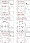 |
Fig. A.1. Left panels: Evolution of the Stokes parameters, polarization degree and angle. Top-right panel: q − u plane. Weighted mean of the source observations (black circles) calculated yearly and of the field stars (red cross). Bottom-right panel: EDF of measured polarization using all data points (black line) or the weighted averaged points (red line) compared with expected (theoretical) CDF of polarization measurements (blue line). |
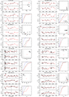 |
Fig. A.1. Continued. |
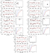 |
Fig. A.1. Continued. |
Appendix B: Extinction curves
This appendix shows the extinction curves for each individual target.
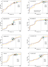 |
Fig. B.1. Extinction as a function of distance in the direction of the targets. The turquoise circle represents the target, while the black circles correspond to the field stars that were used to correct for ISM polarization. |
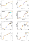 |
Fig. B.1. Continued. |
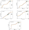 |
Fig. B.1. Continued. |
Appendix C: Sky charts of field stars
Sky charts of the targets. The field of view is 12.5 × 12.5 arcmin. North is up, East is left. The target is marked in red, while the field stars are marked with blue circles.
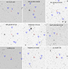 |
Fig. C.1. Sky charts with the identification of the target (red lines) and the field stars (blue circles). |
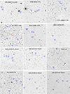 |
Fig. C.1. Continued. |
All Tables
Polarization degree during low-optical states (including disk-loss events) and from field-star analysis.
All Figures
|
Fig. 1. Left: Evolution of the Stokes parameters, polarization degree and angle. Top right: q − u plane. Weighted mean of the source observations (black circles), calculated yearly, and of the field stars (red cross). Bottom right: Empirical distribution function (EDF) of measured polarization using all data points (black line) or the weighted averaged points (red line) compared with expected cumulative distribution function (CDF) of polarization measurements (blue line). The data shown correspond to the BeXB RX J0146.9+6121. |
| In the text | |
|
Fig. 2. Two representative examples of extinction as a function of distance (data from Green et al. 2019). Data points mark the assumed locations of the stars on the extinction curve, based on their distances; they do not imply extinction values. Distances are from Bailer-Jones et al. (2021). The turquoise circle represents the BeXB, the black circles show the field stars used for the ISM correction, and the blue circles correspond to other field stars. We also indicate the polarization degree (PD) of the field stars. The vertical dashed line marks the region of uncertain extinction. |
| In the text | |
|
Fig. 3. Polarization degree and angle near a major (type II) X-ray outburst. The vertical dashed lines indicate the peak of the X-ray outburst. |
| In the text | |
|
Fig. 4. Maximum intrinsic polarization degree as a function of distance (left) and orbital period (right), excluding the outlier EXO 2030+375. The red point corresponds to the Be/γ-ray binary RX J0240.4+6112/LS I +61303. |
| In the text | |
|
Fig. 5. Normalized histogram of the maximum intrinsic polarization (corrected for the ISM) for our BeXB sample, excluding the outlier EXO 2030+375, compared with the polarization distribution of classical Be stars of similar spectral type (data from Yudin 2001). The Y axis is computed so that the total area under the histogram equals 1. |
| In the text | |
|
Fig. A.1. Left panels: Evolution of the Stokes parameters, polarization degree and angle. Top-right panel: q − u plane. Weighted mean of the source observations (black circles) calculated yearly and of the field stars (red cross). Bottom-right panel: EDF of measured polarization using all data points (black line) or the weighted averaged points (red line) compared with expected (theoretical) CDF of polarization measurements (blue line). |
| In the text | |
|
Fig. A.1. Continued. |
| In the text | |
|
Fig. A.1. Continued. |
| In the text | |
|
Fig. B.1. Extinction as a function of distance in the direction of the targets. The turquoise circle represents the target, while the black circles correspond to the field stars that were used to correct for ISM polarization. |
| In the text | |
|
Fig. B.1. Continued. |
| In the text | |
|
Fig. B.1. Continued. |
| In the text | |
|
Fig. C.1. Sky charts with the identification of the target (red lines) and the field stars (blue circles). |
| In the text | |
|
Fig. C.1. Continued. |
| In the text | |
Current usage metrics show cumulative count of Article Views (full-text article views including HTML views, PDF and ePub downloads, according to the available data) and Abstracts Views on Vision4Press platform.
Data correspond to usage on the plateform after 2015. The current usage metrics is available 48-96 hours after online publication and is updated daily on week days.
Initial download of the metrics may take a while.