| Issue |
A&A
Volume 709, May 2026
|
|
|---|---|---|
| Article Number | A171 | |
| Number of page(s) | 7 | |
| Section | Extragalactic astronomy | |
| DOI | https://doi.org/10.1051/0004-6361/202555135 | |
| Published online | 13 May 2026 | |
A possible wave-optical effect in lensed fast radio bursts
1
Indian Institute of Science Education and Research Thiruvananthapuram, 695551 Kerala, India
2
Department of Physics and Astronomy, University of California, Riverside, CA 92521, USA
3
Department of Astronomy, University of California Berkeley, Berkeley, CA 94720, USA
4
Max-Planck-Institut für Radioastronomie, Auf dem Hügel 69, 53121 Bonn, Germany
5
Physik-Institut, University of Zurich, Winterthurerstrasse 190, 8057 Zurich, Switzerland
★ Corresponding authors: This email address is being protected from spambots. You need JavaScript enabled to view it.
, This email address is being protected from spambots. You need JavaScript enabled to view it.
Received:
11
April
2025
Accepted:
1
March
2026
Abstract
Context. Fast radio bursts (FRBs) are enigmatic extragalactic bursts whose properties are still largely unknown, but based on their extremely short duration, they are proposed to have a compact structure, making them candidates for wave-optical effects if gravitationally lensed. If an FRB is lensed into multiple-image bursts at different times by a galaxy or cluster, a likely scenario is that only one image is detected because the others fall outside the survey area and time frame.
Aims. We explore the FRB analog of quasar microlensing, namely the collective microlensing by stars in the lensing galaxy, now including wave optics. The eikonal regime is applicable here.
Methods. We studied the voltage (rather than the intensity) in a simple simulation consisting of (a) microlensing stars and (b) plasma scattering by a turbulent interstellar medium.
Results. The autocorrelation of the voltage shows peaks (at a separation on the order of microseconds) corresponding to wave-optical interference between lensed micro-images. The peaks are frequency dependent when plasma-scattering is significant. While qualitative and still in need of more realistic simulations, the results suggest that a strongly lensed FRB might be identified from a single image.
Conclusions. Macro-lensed FRBs might be recognizable from a microlensing signature.
Key words: gravitational lensing: micro
© The Authors 2026
 Open Access article, published by EDP Sciences, under the terms of the Creative Commons Attribution License (https://creativecommons.org/licenses/by/4.0), which permits unrestricted use, distribution, and reproduction in any medium, provided the original work is properly cited.
This article is published in open access under the Subscribe to Open model. This email address is being protected from spambots. You need JavaScript enabled to view it. to support open access publication.
1. Introduction
Ever since the discovery of an unprecedented signal in an archival radio time series by D. J. Narkevic, then an undergraduate researcher, and the interpretation of that signal as an exceptionally bright extragalactic radio transient (Lorimer et al. 2007), the interest in fast radio bursts (FRBs) has steadily increased (Ng 2023; Lorimer et al. 2024). Fast radio bursts last from microseconds to milliseconds and are characterized by very high dispersion measures that indicate cosmological distances, which implies that they are brighter by 10 to 12 orders of magnitude than radio sources within the Milky Way. They are also very common across the sky; an FRB is expected once every ten seconds (Keane & Petroff 2015; Champion et al. 2016). While early single-dish telescopes such as the Parkes and Arecibo telescopes could detect only a few FRBs, the Canadian Hydrogen Intensity Mapping Experiment (CHIME, see CHIME/FRB Collaboration 2018) with its much larger field of view has detected hundreds (CHIME/FRB Collaboration 2021). Observation of additional signals from FRB121102 led to the understanding that FRBs can have a repeating nature (Spitler et al. 2014, 2016), showing that they are not always cataclysmic events. While follow-up observations with single-dish telescopes were difficult, CHIME has reported that a few percent of the detected FRBs have a repeating feature (Andersen et al. 2020, 2023), and a subset of these have periodic activity windows. Repeating FRBs have wide-ranging properties that peak at different frequencies and have multiple components (e.g., Chatterjee et al. 2017; Tendulkar et al. 2017). In many cases, they can be precisely localized, and in these cases, the intergalactic medium can be studied.
The rapid time variation in FRBs indicates small intrinsic sizes. This would imply that FRB signals are spatially coherent, which would lead to interference effects in cases of gravitational lensing. Several authors (Eichler 2017; Katz et al. 2020; Kader et al. 2022; Leung et al. 2022; Kumar & Beniamini 2023) have considered the possible lensing of FRBs by black holes or other compact masses. These works also noted a significant complication, which is frequency-dependent plasma lensing by the interstellar medium in the host galaxy and in the Milky Way.
Wucknitz et al. (2021) considered multiple images in galaxy and cluster lensing and drew attention to the prospect of measuring the redshift drift when time delays from FRB repeaters are observed. One of the potential complications they noted is the collective microlensing by stars in the lensing galaxy or cluster. Lewis (2020) studied the expected effect of microlensing on lensing time delays. A difficulty in finding these multiple-image systems is that a survey may detect one image from a system, but miss the others because the survey pointing has moved to a different part of the sky. Since about one in 1000 high-redshift objects is lensed into multiple images, it is plausible that a strongly lensed FRB has already been observed without being recognizable as such.
We carry out some simple simulations of wave optics in collective microlensing by stars. That is, we combine ideas from the works mentioned in the previous two paragraphs. The result suggests that collective microlensing by stars imprints an observable signature on a lensed FRB, even without more than one detected image.
2. Gravitational lensing with eikonal optics
The formation of multiple images of a source by an intervening gravitational field, commonly called strong lensing, occurs in two very different regimes. One regime involves stellar or planetary-scale masses in or near the Milky Way (see e.g., Mróz et al. 2024). The other regime is over cosmological distances, and this situation is more relevant to FRBs. The theory was introduced in several places, such as Meneghetti (2022) and Saha et al. (2024) in recent years, with Leung et al. (2023) covering the wave-optics part in detail. We summarize the essential points below.
2.1. Images and magnification
Strong lensing involves a combination of two very different scales. One scale are distances in the combination
 (1)
(1)
Here, Dd and Ds are angular diameter distances from the observer to the deflector (lens) and the source, respectively, and Dds is the angular diameter distance from the deflector to the source. 𝒟/c is on the order of the total light travel time. The second scale is
 (2)
(2)
which is always ≪𝒟/c. Image separations are on the scale of the Einstein radius, given by
 (3)
(3)
𝒯 itself is the typical difference in light travel time between images, known as time delays. For multiple images to form, θE needs to fit within the angular size of the mass itself. This becomes more common for larger distances because θE ∝ 𝒟−1/2, whereas the angular size ∝Dd−1.
There are separated subfields of lensing, corresponding to different scales of 𝒯 and θE.
-
For cluster lenses (for a recent review see Natarajan et al. 2024), where 𝒯 is years to decades, and θE reaches the arcminute scale.
-
For galaxy lenses (see Shajib et al. 2024, for a recent review), 𝒯 is days to months, while θE is on the arcsecond scale.
-
For the collective lensing by stars within a strongly lensing galaxy or cluster, which splits the individual images formed (the so-called macro-images) into many micro-images. Here, 𝒯 is on the microsecond scale, and θE is on the micro-arcsecond scale. The phenomenon is of interest for sources that are small enough, and it has been extensively studied for lensed quasars (see e.g., Vernardos et al. 2024). The scale of θE is too small to resolve the images, but changes in brightness resulting from transverse motion are observable. It is potentially even more interesting for FRBs because of the smaller source size.
Lensing often uses the arrival-time surface. We considered the possible light travel time for a photon originating at an angular position β, which is deflected and then arrives from a direction θ. The arrival time can be scaled to a dimensionless form as
 (4)
(4)
and can be expressed as the sum of geometric and gravitational delays. For a single point mass, the dimensionless arrival time is
 (5)
(5)
Contributions for more masses can be summed or integrated. For collective microlensing by N equal masses, we have
 (6)
(6)
with ψB representing a background contribution due to all other masses. By Fermat’s principle, images form, for which
 (7)
(7)
gives the lens equation
 (8)
(8)
The deflection of light rays by large-scale gravitational lenses such as galaxies or galaxy clusters is described by the macrolensing potential, denoted by ψB(θ) in Eq. (8). The macrolensing potential governs the overall distortion of light rays originating from background sources. The deflection angle at the angular position θ on the sky is given by the gradient of the potential, ∇ψB(θ). A Taylor expansion of the deflection angle at leading order yields a constant term corresponding to an effective shift in the apparent source position from β. The next-order term, involving the second derivative of the potential (or the first derivative of the deflection angle), captures the local stretching and shearing of the arrival-time surfaces. Microlensing simulations (going back to Paczynski 1986) generally assume constant stretching and shearing, neglecting higher-order effects. For simpler simulations designed for illustrative purposes (e.g., Vernardos et al. 2024), the background potential may be neglected altogether. Its omission does not qualitatively affect our primary results.
By visualizing the arrival-time surfaces τ(θ; β), it is possible to visualize three types of images formed at locations in which the surface has zero gradient. If there is no lens, then there is a minimum at the point θ = β surrounded by a parabolic well. A circular lens directly aligned with the source replaces this parabola with a hill surrounded by a circular valley. However, if this is not the case, the valley is asymmetric, with a bowl on one side. The more complex the mass distribution, the greater the number of valleys and hills that appear, leading to maxima and minima. Another set of images is formed by saddle points that also satisfy the zero-gradient condition.
The Hessian of τ(θ) determines how quickly or slowly we are moved off-source by a change in θ. By defining (M−1)ij ≡ ∂i∂jτ(θ) as the inverse magnification matrix, it can explain the lensing caused by many small and finite sources as
 (9)
(9)
The scalar magnification μ(θ) is given by
 (10)
(10)
The magnification is negative for images at saddle points.
2.2. Wave optics in the eikonal regime
While geometric optics is a good enough approximation for most astronomical sources that are large enough so radiation from different parts of the source reaches the observer incoherently, wave optics applies to small sources that are far away. This applies to gravitational waves (e.g., Dai et al. 2020; Mishra et al. 2021). The case of FRBs is simpler because of the much higher frequencies, enabling an eikonal approximation.
An unlensed narrow-band signal of the form
 (11)
(11)
results in a lensed signal
 (12)
(12)
where we defined
 (13)
(13)
 (14)
(14)
and τk corresponds to the kth micro-image. It is therefore straightforward to calculate the lensed signal from a large number of micro-images.
2.3. Plasma scattering
In addition to gravitational lensing, an important obstacle in the radio domain is the scattering caused by turbulence in the interstellar medium. This depends on the electron density and amounts to an additional time delay that is proportional to ν−2. This produces deflections similar to those produced by microlensing, forming a large number of images that can interfere with each other. Due to their extragalactic nature, FRBs can be affected by scattering in the lens galaxy and the intergalactic medium apart from the Milky Way. This would be most serious if the lensing galaxy were gas rich, but as most lensing galaxies are elliptical, a comparatively low level of plasma scattering is expected (Wucknitz et al. 2021).
To model plasma scattering, we add the term
 (15)
(15)
to the scaled time-delay (6). Here, p(θ) denotes a turbulent field normalized as
 (16)
(16)
The strength is then set by ν0, which we can understand as the frequency for which plasma scattering contributes as much as a star microlensing on its own. Gravitational lensing dominates in the ν ≫ ν0 regime. Plasma scattering becomes progressively less important with an increase in ν.
To produce a realization of p(θ), we let its Fourier transform be a power law with small-scale and large-scale cutoffs (cf. Eq. 1 in Armstrong et al. 1995). The Fourier component corresponding to
 (17)
(17)
is given an amplitude of
 (18)
(18)
and a random phase. Here, l0 and L0 are the grid size and field size, respectively, which act as the small-scale and large-scale cutoffs. Since an integral along the line of sight is desired, we set qz = 0. The real part of p(θ) was taken and normalized according to Eq. (16). Fig. 1 shows an example realization of p(θ).
 |
Fig. 1. Time delay due to turbulent ISM, normalized according to Eq. (16). The spatial scale is the same as the microlensing fields in left panels in Figs. 2–4 below. |
The grid size for the simulation was chosen as 1024 × 1024, with each point corresponding to one Einstein radius. The physical distance corresponding to the Einstein radius (Eq. 3) is given by
 (19)
(19)
and is on the order of some milliparsecs or light days. The small-scale cutoff l0 is roughly 10−2 𝒟 θE and the large-scale cutoff L0 corresponds to 10 𝒟 θE. The region of interest in which we assumed microlensing to take place lies between these two scales, and the turbulence was expected to be scale free.
3. A simple simulation
We present in this section the results obtained from the effects of macrolensing, microlensing, and a turbulent interstellar plasma on the FRB signal.
We start with an illustrative microlensing simulation from the recent literature (Vernardos et al. 2024, – see especially their Figs. 4 and 6). The simulation had 50 equal point-mass lenses, whose Einstein radii covered ∼40% of the image plane (κ* ∼ 0.4 in the usual notation). This assumes that the stellar mass is a significant contributor to the total lensing mass, but the stellar mass need not be dominant. More elaborate simulations have many thousands of particles and include a smooth tidal field (known as external shear), but the qualitative properties of micro-images are already present in this example. Of particular interest is a cluster of four bright micro-images, two minima and two saddle points.
To the scaled time delay (Eq. 6) corresponding to the above lensing system, we added the plasma scattering term (Eq. 15) with adjustable ν0. The micro-images were found using a simple recursive grid search. A random coherent signal spectrum S(ν) was generated, and this signal was lensed according to Eqs. (12–14). The lensed signal was then auto-correlated. Using Eqs. (12–14), we derived the autocorrelation to be
 (20)
(20)
C(t) clearly has peaks when t = τk − τj. For a theoretical understanding, we distinguish between the real and imaginary parts of the autocorrelation, even though they may not be distinguishable in practice.
3.1. Lensing-dominated regime
Fig. 2 illustrates this regime. The left panel in Fig. 2 is equivalent to Fig. 6 (except for some details) in Vernardos et al. (2024). The micro-images are as follows:
-
Two bright minima with time delays (say) τ0, τ1,
-
Two bright saddle points with time delays τ2, τ3, and
-
Faint saddle points with time delays τ4, τ5, τ6, and so on.
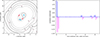 |
Fig. 2. Left. Micro-images in the lensing-dominated regime. The black dots mark stellar masses. The gray curves show the arrival-time contours. Ellipses show micro-images (blue for minima, and red for saddle points). Right. Autocorrelation signals are shown in blue for the real part and in magenta for the imaginary part. A tanh activation function has been applied to reduce the contrast between the lines. |
An important property of collective microlensing by stars (see e.g., Nityananda & Ostriker 1984; Saha & Williams 2011) is that the observable signal is completely dominated by a few bright micro-images, while the faint micro-images, though much more numerous, contribute very little to the light. In this example, the two bright minima and two bright saddle points all have |μk|∼1, with the remaining images being fainter by some orders of magnitude. Thus, only the first four micro-images would be observationally relevant. For a theoretical understanding, however, we continued to consider the first few faint micro-images as well.
The right panel in Fig. 2 shows the autocorrelation (Eq. 20) of the lensed signal in the left panel of the same figure. Each line in the autocorrelation (after the line at zero delay) is associated with a pair of micro-images. The strong lines are associated with pairs of bright micro-images. Blue and magenta indicate the real and imaginary parts, which are associated with image pairs of like and opposite parity respectively. These appear
-
at τ1 − τ2 between two opposite-parity images,
-
at τ3 − τ2 and τ1 − τ0, which happen to be almost equal, between like-parity images,
-
at τ2 − τ0 and τ3 − τ1, which again happen to be nearly equal between like-parity images, and
-
at τ3 − τ0 again between opposite-parity images.
Then, there is a repeating pattern of four lines, as a faint micro-image is paired with the four bright micro-images
-
at τk − τ0 and τk − τ1 between opposite-parity images, and
-
at τk − τ2 and τk − τ3 between like-parity images
for k = 4, 5, 6 and so on, which continues beyond the figure. These are only of theoretical interest, as there is no prospect of observing them. There are also some even fainter lines
-
at τk − τj
for k, j > 3, corresponding to pairs of faint micro-saddles.
The magenta lines in Fig. 2 all happen to be negative. The reason for this can be seen by referring to Eq. (20) for the autocorrelation. Since the figure shows positive t, it implies τk > τj at the peaks. The magenta lines come from cases where τj is a minimum and τk is a saddle point. Since all the saddle points arrive later than all the minima, τk always corresponds to a saddle point, and the associated αk* factor makes the imaginary part negative. If any saddle points arrived earlier than a minimum, a positive magenta line would appear.
3.2. The effect of plasma scattering
We now show the effect of adding the plasma-scattering term (Eq. 15). Fig. 2 discussed above already had a small plasma-scattering contribution, corresponding to ν = 20 ν0. In the next two figures, we gradually reduce ν. In these figures, we also zoom in to highlight the bright micro-images and the autocorrelation peaks between them.
Fig. 3 shows that down to ν = 10 ν0, there is only a slight shift in the autocorrelation peaks; that is, plasma scattering is not significant. At ν = 8 ν0, however, a qualitative change appears. The bright micro-minimum initially at τ2 splits into three bright micro-images (two minima and a saddle point). Accordingly, more lines appear in the autocorrelation.
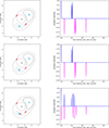 |
Fig. 3. Arrival-time contours (left) and autocorrelation signals (right) for intermediate-frequency signals at ν/ν0 of 13 (top row), 10 (middle row), and 8 (bottom row). |
In Fig. 4, the frequency is lowered in steps to 5 ν0. The saddle point initially at τ3 now splits into three images, while the triplet near τ2 that formed at ν = 8 ν0 separates out a little. This is the first example of a minimum (near τ3) that is later than a saddle point (near τ2), leading to a positive imaginary part.
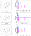 |
Fig. 4. Arrival-time contours (left) and auto-correlation signals (right) for low-frequency signals, ν/ν0 being 7 (top row), 6 (middle row), and 5 (bottom row). The slight wiggles in the curves in the bottom left panel are due to small-scale fluctuations from plasma scattering. |
We thus see the familiar theme that the observable is independent of frequency when gravitational lensing dominates and depends on frequency when the interaction with the medium is strong.
4. Observational aspects
The details of the observations and data processing go beyond the scope of this theoretically motivated paper, but we need to understand the chance of an actual detection of microlensing signatures.
Fast radio bursts are basically found as peaks in time series of the detected power over long observations. In reality, the data are channeled to form dynamic (time-resolved) spectra, to be able to correct for dispersion from the interstellar medium, and to distinguish astrophysical bursts from artificial interference. For the microlensing analysis, the original voltage signal S(t), or equivalently, S(ν), is needed for the duration of the burst to form the autocorrelation according to Eq. (20). Such data are now recorded on a regular basis by CHIME and ASKAP, but also by telescopes such as the Effelsberg telescope, which are used for follow-up observations of repeating bursts.
Because the central peak at C(0) corresponds to the integrated detected power, we know it to be well above the noise level. Microlensing-induced peaks at τk − τj (for k > j ≥ 0) are proportional to |αjαk| or the geometric mean of the intensities of the corresponding micro-images. This can be compared to the central peak, which is effectively proportional to ∑j|αj|2 (the sum of all intensities), after averaging over frequency.
For the image configuration in Fig. 2, the ratio is 0.29 for the highest microlensing peak compared to C(0), which is detectable if the initial FRB detection has a sufficiently high signal-to-noise ratio. The actual detection analysis requires a thorough statistical analysis of false-detection rates, taking into account the number of trial lags.
The frequency (here, ν0) at which plasma scattering and lensing become comparable is unknown. When ν0 is lower than the GHz scale of FRB observations, the wave-optical effect discussed here will be observable. Otherwise, the effect will be washed out by plasma scattering. The overall delay due to plasma scattering will be comparable to the observed dispersion (which is about one second). This is vastly longer than the microsecond scale delays due to individual stars, but tiny compared to the overall time delay of all the lensing mass (time delays in galaxy lensing are months). What is relevant is whether the plasma-scattering term varies on the microsecond scale over the transverse scale of microlensing (which is micro-arcseconds or picoradians). Equivalently, the question is whether the small-scale cutoff of the turbulent plasma is smaller than the microlensing scale.
The scattering delays can depend on the Galactic latitude, with low Galactic latitudes showing stronger effects in general (Wucknitz et al. 2021). For latitudes above 20°, a scattering delay at 1.4 GHz is always shorter than 1 microsecond. Additional constraints on small-scale plasma fluctuations come from secondary-spectrum measurements (Sprenger et al. 2021, Fig. 4). Except for a special case at 1 millisecond, most scattering features have delays of about a few hundred microseconds at 330 MHz. As typical delays scale as ∼ν−4.4, even the strongest 1 millisecond feature would be ∼1.7 microseconds at 1.4 GHz – a case of strong scattering. Characteristic scattering angles at about 330 MHz are also found to be ∼30 mas, which scale with frequency as ν−2.2, implying angular broadening of ∼1 mas at 1.4 GHz (Sprenger et al. 2021, Fig. 9). This means that microseconds and mas are appropriate order-of-magnitude estimates at 1.4 GHz. In the lensing galaxy however, scattering can be substantially stronger as the delays scale with distance. In such environments, plasma-phase fluctuations might approach or exceed microlensing scales and might suppress wave-optics features.
5. Conclusions
Based on the above simulation, we make the following interpretation. When a lensed FRB is smaller than the Fresnel scale, which is (𝒟 c/ν)1/2 ∼ 10 au for GHz observations, and when it is moreover not smeared too much by the contents of the interstellar or intergalactic medium (making it a coherent source), then a single macro-image can be used for recognizing the lens. The well-known fine time structure in FRBs indicates that they are small enough to be coherent. Since most strongly lensing galaxies are elliptical, lensed FRBs would be exposed to the low end of plasma scattering.
It would be interesting to examine autocorrelated voltage time series at different frequencies (as simulated in Kader et al. 2024, Figs. 11–12) for a sample of FRBs observed in different parts of the sky, and thus, in different regions of the Milky Way. While not expected to yield any lensed specimens, even a small sample would give an indication how strong plasma scattering is through the frequency dependence of the autocorrelation. If there are frequency-dependent peaks in the autocorrelation at all frequencies, it would not be possible to separate the contributions of gravitational lensing and plasma scattering. If autocorrelation peaks are absent at some (high) frequencies, the outlook for finding lenses by this method would be positive.
References
- Andersen, B. C., Bandura, K. M., Bhardwaj, M., et al. 2020, Nature, 587, 54 [NASA ADS] [CrossRef] [Google Scholar]
- Andersen, B. C., Bandura, K., Bhardwaj, M., et al. 2023, ApJ, 947, 83 [NASA ADS] [CrossRef] [Google Scholar]
- Armstrong, J. W., Rickett, B. J., & Spangler, S. R. 1995, ApJ, 443, 209 [Google Scholar]
- Champion, D. J., Petroff, E., Kramer, M., et al. 2016, MNRAS, 460, L30 [Google Scholar]
- Chatterjee, S., Law, C. J., Wharton, R. S., et al. 2017, Nature, 541, 58 [NASA ADS] [CrossRef] [Google Scholar]
- CHIME/FRB Collaboration (Amiri, M., et al.) 2018, ApJ, 863, 48 [NASA ADS] [CrossRef] [Google Scholar]
- CHIME/FRB Collaboration (Amiri, M., et al.) 2021, ApJS, 257, 59 [NASA ADS] [CrossRef] [Google Scholar]
- Dai, L., Zackay, B., Venumadhav, T., Roulet, J., & Zaldarriaga, M. 2020, Search for Lensed Gravitational Waves Including Morse Phase Information: An Intriguing Candidate in O2 [Google Scholar]
- Eichler, D. 2017, ApJ, 850, 159 [Google Scholar]
- Kader, Z., Leung, C., Dobbs, M., et al. 2022, Phys. Rev. D, 106, 043016 [Google Scholar]
- Kader, Z., Dobbs, M., Leung, C., Masui, K. W., & Sammons, M. W. 2024, Phys. Rev. D, 110, 123027 [Google Scholar]
- Katz, A., Kopp, J., Sibiryakov, S., & Xue, W. 2020, MNRAS, 496, 564 [Google Scholar]
- Keane, E. F., & Petroff, E. 2015, MNRAS, 447, 2852 [NASA ADS] [CrossRef] [Google Scholar]
- Kumar, P., & Beniamini, P. 2023, MNRAS, 520, 247 [Google Scholar]
- Leung, C., Kader, Z., Masui, K. W., et al. 2022, Phys. Rev. D, 106, 043017 [Google Scholar]
- Leung, C., Jow, D., Saha, P., et al. 2023, arXiv e-prints [arXiv:2304.01202] [Google Scholar]
- Lewis, G. F. 2020, MNRAS, 497, 1583 [Google Scholar]
- Lorimer, D. R., Bailes, M., McLaughlin, M. A., Narkevic, D. J., & Crawford, F. 2007, Science, 318, 777 [Google Scholar]
- Lorimer, D. R., McLaughlin, M. A., & Bailes, M. 2024, Astrophys. Space Sci., 369 [Google Scholar]
- Meneghetti, M. 2022, Introduction to Gravitational Lensing: With Python Examples [Google Scholar]
- Mishra, A., Meena, A. K., More, A., Bose, S., & Bagla, J. S. 2021, MNRAS, 508, 4869 [Google Scholar]
- Mróz, P., Udalski, A., Szymański, M. K., et al. 2024, ApJ, 976, L19 [Google Scholar]
- Natarajan, P., Williams, L. L. R., Bradač, M., et al. 2024, Space Sci. Rev., 220, 19 [CrossRef] [Google Scholar]
- Ng, C. 2023, A brief review on Fast Radio Bursts [Google Scholar]
- Nityananda, R., & Ostriker, J. P. 1984, J. Astrophys. Astron., 5, 235 [Google Scholar]
- Paczynski, B. 1986, ApJ, 301, 503 [NASA ADS] [CrossRef] [Google Scholar]
- Saha, P., & Williams, L. L. R. 2011, MNRAS, 411, 1671 [Google Scholar]
- Saha, P., Sluse, D., Wagner, J., & Williams, L. L. R. 2024, Essentials of strong gravitational lensing [Google Scholar]
- Shajib, A. J., Vernardos, G., Collett, T. E., et al. 2024, Space Sci. Rev., 220, 87 [CrossRef] [Google Scholar]
- Spitler, L. G., Cordes, J. M., Hessels, J. W. T., et al. 2014, ApJ, 790, 101 [NASA ADS] [CrossRef] [Google Scholar]
- Spitler, L. G., Scholz, P., Hessels, J. W. T., et al. 2016, Nature, 531, 202 [NASA ADS] [CrossRef] [Google Scholar]
- Sprenger, T., Wucknitz, O., Main, R., Baker, D., & Brisken, W. 2021, MNRAS, 500, 1114 [Google Scholar]
- Tendulkar, S. P., Bassa, C. G., Cordes, J. M., et al. 2017, ApJ, 834, L7 [NASA ADS] [CrossRef] [Google Scholar]
- Vernardos, G., Sluse, D., Pooley, D., et al. 2024, Space Sci. Rev., 220, 14 [NASA ADS] [CrossRef] [Google Scholar]
- Wucknitz, O., Spitler, L. G., & Pen, U.-L. 2021, A&A, 645, A44 [NASA ADS] [CrossRef] [EDP Sciences] [Google Scholar]
All Figures
|
Fig. 1. Time delay due to turbulent ISM, normalized according to Eq. (16). The spatial scale is the same as the microlensing fields in left panels in Figs. 2–4 below. |
| In the text | |
|
Fig. 2. Left. Micro-images in the lensing-dominated regime. The black dots mark stellar masses. The gray curves show the arrival-time contours. Ellipses show micro-images (blue for minima, and red for saddle points). Right. Autocorrelation signals are shown in blue for the real part and in magenta for the imaginary part. A tanh activation function has been applied to reduce the contrast between the lines. |
| In the text | |
|
Fig. 3. Arrival-time contours (left) and autocorrelation signals (right) for intermediate-frequency signals at ν/ν0 of 13 (top row), 10 (middle row), and 8 (bottom row). |
| In the text | |
|
Fig. 4. Arrival-time contours (left) and auto-correlation signals (right) for low-frequency signals, ν/ν0 being 7 (top row), 6 (middle row), and 5 (bottom row). The slight wiggles in the curves in the bottom left panel are due to small-scale fluctuations from plasma scattering. |
| In the text | |
Current usage metrics show cumulative count of Article Views (full-text article views including HTML views, PDF and ePub downloads, according to the available data) and Abstracts Views on Vision4Press platform.
Data correspond to usage on the plateform after 2015. The current usage metrics is available 48-96 hours after online publication and is updated daily on week days.
Initial download of the metrics may take a while.