| Issue |
A&A
Volume 709, May 2026
|
|
|---|---|---|
| Article Number | A42 | |
| Number of page(s) | 9 | |
| Section | Astrophysical processes | |
| DOI | https://doi.org/10.1051/0004-6361/202557808 | |
| Published online | 30 April 2026 | |
The elusive cyclotron line in 4U 1901+03: Hidden, yet present
1
INAF – IASF-Palermo, Via Ugo La Malfa 153, 90146 Palermo, Italy
2
Department of Astronomy, University of Geneva, Chemin d’Écogia 16, 1290 Versoix, Switzerland
3
Dr. Karl Remeis-Observatory and Erlangen Centre for Astroparticle Physics, Friedrich-Alexander Universität Erlangen-Nürnberg, Sternwartstr. 7, 96049 Bamberg, Germany
4
Dipartimento di Fisica e Chimica Emilio Segrè, Università di Palermo, Via Archirafi 36, 90123 Palermo, Italy
5
Department of Physics, National and Kapodistrian University of Athens, University Campus Zografos, GR 15784 Athens, Greece
6
European Space Agency (ESA), European Space Astronomy Centre (ESAC), Camino Bajo del Castillo s/n, 28692 Villanueva de la Cañada, Madrid, Spain
7
INAF – Osservatorio Astronomico di Roma, Via Frascati 33, I-00078 Monte Porzio Catone, (RM), Italy
★ Corresponding author: This email address is being protected from spambots. You need JavaScript enabled to view it.
Received:
23
October
2025
Accepted:
15
March
2026
Abstract
Context. Cyclotron resonant scattering features in accreting X-ray pulsars are often difficult to detect, especially when shallow or variable. Recent studies have shown that combining spectral and timing analyses enhances their detectability.
Aims. We investigated the evolution of energy-resolved pulse profiles of the X-ray pulsar 4U 1901+03 during its 2019 giant outburst, focusing on the 30–40 keV range where there have been disputed claims of a cyclotron line detection and its properties.
Methods. We analysed four NuSTAR observations of 4U 1901+03 at different luminosities. We studied energy-resolved pulse profiles using harmonic decomposition, cross-correlation analysis, energy–phase maps, and pulsed-fraction spectra, and we used Bayesian spectral modelling to assess the presence and properties of a cyclotron line.
Results. We detected significant spectral–timing variability in the 30–40 keV range, which became stronger at lower luminosities. We found a pronounced drop in the pulsed fraction near ≈35 keV only in the lowest accretion state and in the first harmonic of one intermediate-luminosity observation. Adopting a Bayesian informative approach on the spectral parameters, we find evidence of a cyclotron line in all the examined energy spectra, with an average centroid energy of Ecyc ≈ 32 keV, varying by only ≈1.6%, with anti-correlation between line depth and luminosity. We show that a combined spectral-timing approach is more sensitive than phase-averaged spectroscopy to shallow cyclotron features. The luminosity-dependent evolution of pulse profiles and the depth of the cyclotron line point to a drastic change in the emission geometry and the accretion flow structure.
Key words: accretion / accretion disks / stars: neutron / X-rays: binaries / X-rays: individuals: 4U 1901+03
© The Authors 2026
 Open Access article, published by EDP Sciences, under the terms of the Creative Commons Attribution License (https://creativecommons.org/licenses/by/4.0), which permits unrestricted use, distribution, and reproduction in any medium, provided the original work is properly cited.
This article is published in open access under the Subscribe to Open model. This email address is being protected from spambots. You need JavaScript enabled to view it. to support open access publication.
1. Introduction
Be X-ray binaries (BeXRBs) represent the most numerous subclass of high-mass X-ray binaries, typically consisting of a neutron star in an eccentric orbit around a young, massive Be star. These systems are characterised by transient high-luminosity X-ray outbursts, often triggered by the interaction of the compact object with the circumstellar decretion disk of the companion (see e.g. Reig 2011). During these events, the neutron star accretes material along magnetic field lines, forming accretion columns where the dynamics are governed by the interplay between the mass accretion rate (Ṁ) and the strong magnetic field (B ≈ 1012 − 13 G). The resulting emission pattern is fundamentally determined by the critical luminosity, Lcrit (Basko & Sunyaev 1976; Becker et al. 2012; Mushtukov et al. 2015; Mushtukov & Tsygankov 2022): at L < Lcrit, the flow is decelerated by Coulomb interactions (sub-critical regime), leading to a pencil-beam pattern dominated by emission escaping along the magnetic axis. Conversely, at L > Lcrit (super-critical regime), a radiation-dominated shock halts the infalling plasma, and photons diffuse through the column’s lateral walls in a fan-beam dominated pattern. The emerging spectrum, shaped by thermal and bulk Comptonization (Becker & Wolff 2022), is further modified by relativistic effects (gravitational redshift and light bending) and by the possible presence of cyclotron resonant scattering features (CRSFs). These absorption-like features are primary diagnostics of the magnetic field strength and the geometry of the emitting region (Staubert et al. 2019; Schwarm et al. 2017). However, phase-averaged spectral analysis often suffers from the mixing of different spin-phase contributions, complicating the interpretation of the underlying beam pattern.
The dependence of the emission pattern on luminosity and energy results in complex, multi-peaked pulse profiles (PPs) that evolve non-trivially across different regimes (see Alonso-Hernández et al. 2022, for an overview). This variability complicates phase-averaged spectral analysis, as it inevitably mixes different physical contributions. To decouple these effects, a combined timing and spectral approach might alleviate spectral model degeneracy. As demonstrated by Ferrigno et al. (2023, hereafter FDA23), the pulsed fraction spectrum (PFS), derived from high-resolution energy-resolved pulse profiles, can isolate local substructures associated with spectral features such as the iron Kα line and CRSFs. This technique has successfully identified cyclotron line wings in V0332+53 (D’Aì et al. 2025) and helped constrain the spin-phase modulation of the CRSF depth in 4U 1538−52 through physical modelling (Sokolova-Lapa et al. 2023; Maniadakis et al. 2025)
In this work, we applied and extended the method presented in FDA23 to analyse the 2019 giant outburst of 4U 1901+03, a BeXRB with spin period Pspin ≈ 2.7 s (Galloway et al. 2005), discovered thanks to the Uhuru satellite (Forman et al. 1976) during a giant outburst. Its orbital period is ≈22.58 d, with an almost circular orbit (e = 0.0144) and a projected semi-major axis of axsin i = 104.236 lt-s (Tuo et al. 2020). Since its discovery, it has undergone four major outbursts, the last one in 2019, of which we analysed the NuSTAR data. The structure of the paper is as follows. In Sect. 2 we describe the data processing, extract the properties of the pulse profiles (Sect. 2.2), and their pulse fraction spectra (Sect. 2.3), and describe how they connect the high energy spectra of each observation (Sect. 2.4). The discussion is in Sect. 3, while the summary and conclusions are in Sect. 4.
2. Analysis
2.1. Data reduction and filtering
Our dataset consists of four NuSTAR observations, shown in Fig. 1 together with the 2019 outburst observed by Swift/BAT (15 − 50 keV)1. One observation was performed before the peak of the outburst and the others were taken during the descending phase; we refer to these observations as Obs A to Obs D hereafter.
 |
Fig. 1. Swift/BAT light curve of the 2019 giant outburst (15–50 keV), rate in count s−1 cm−2; vertical lines mark the epochs of the four NuSTAR observations. |
We performed data reduction following standardized procedures wrapped in the Python module NUSTARPIPELINE2 presented in FDA23. Here, we outline the main steps.
We first obtained calibrated level 2 event files from the Modules (FPMA and FPMB) and defined the source region as the one containing 95% of the source signal, centred on the best known coordinates of 4U 1901+03 (RA, Dec (J2000) = 19:03:39.39, 03:12:15.8); we defined background regions with the same size, located in a detector area free of contaminating sources.
Then, to avoid contamination from flares and/or dips, we analysed the light curve and discarded periods with high source variability, following the same procedure shown in FDA23. We obtained the spin frequency in each observation after barycentric and orbit corrections3 of the event arrival times. We did not detect any spin derivative in any dataset and, therefore, we applied no corrective term. The effective exposures and spin periods are reported in Table 1.
NuSTAR observations.
2.2. Energy-resolved pulse profiles and energy-phase maps
We applied the methods described and presented in FDA23 to compute the energy-resolved pulse profiles, but for this analysis we increased the energy resolution by a factor of three at lower energies (E < 10 keV), where the S/N is higher with respect to higher energies, ending with a total of 131 energy bins in the 2.0–70 keV full band.
We extracted energy-resolved pulse profiles with 20 phase bins and re-binned them in energy to reach a minimum S/N of five. A good visual representation is given through the energy phase maps (hereafter EPM), which illustrate at once the pulse shape variations with energy and phase, as shown in Fig. 2. We show them in the upper panels of Fig. 2 with the phase on the y-axis and the energy on the x-axis (pulse profiles extracted in some representative energy bands for the four datasets are shown in Beri et al. 2021). To better investigate the local variability of the energy-resolved pulse profiles, we employed a moving window cross-correlation (MWCC) technique, designed to track rapid changes between adjacent profiles. We adopted the same method described in FDA23 (see their Eq. (3) and Fig. 3), with the difference that here each energy-resolved profile is compared with a reference profile obtained by averaging the surrounding profiles, excluding the energy bin of interest, within a maximum index distance of w. After some testing, we found that w = 2 provides the most suitable balance between sensitivity to local variations and statistical robustness, allowing us to effectively trace profile changes across the entire energy range. MWCC values are shown in the bottom panels of each plot in Fig. 2. The most important result emerging from these four plots is that they share a common behaviour above 30 keV, where the MWCC values exhibit an abrupt drop. Below this energy, Obs C and D show a high degree of similarity, with MWCC values approximately close to unity, whereas the higher-luminosity observations (A and B) display significant energy-dependent variability in their pulse profiles.
 |
Fig. 2. Energy-phase maps and MWCC with a window of two adjacent bins (see text). For each panel, we chose Nbins = 20 and S/N = 5.0. The colour bar, on the right side of each map, represents the values of the normalised profiles plotted in the map and spans between the minimum and the maximum of the entire map. |
2.3. Pulsed fraction spectra
As shown in FDA23, the parallelism between the energy spectra and the pulsed fraction spectra can be quantified by modelling the latter. We defined a ‘continuum’, described by a polynomial, to trace the general trend of the pulsed fraction spectrum, while local substructures at the energies of the iron Kα line (6.4 keV) and the CRSF were modelled with negative Gaussians, which we referred to as ‘dips’.
We computed the PFS of 4U 1901+03 using the rms definition4 of the pulsed fraction, PFrms which quantifies the variability of each profile relative to its mean. In practice
![Mathematical equation: $$ \begin{aligned} PF_{\mathrm{rms}} = \frac{\sqrt{ \Sigma _{i = 0}^N \left[ (c_i - \bar{c})^2 - \sigma _{c_i}^2 \right] / N}}{\bar{c}} ,\end{aligned} $$](/articles/aa/full_html/2026/05/aa57808-25/aa57808-25-eq1.gif) (1)
(1)
where  is the average count rate for each profile, ci is the normalised count rate in the i phase bins, and σci the corresponding standard deviation. Beyond the global variability traced by the PFS, the harmonic components of the pulse profiles can provide additional insights. In particular, we analysed the energy dependence of the amplitude of the first harmonic, obtained from the Fourier decomposition of each profile, and modelled it in the same way as for the PFS. In Fig. 3 we show the PFS and the spectrum of the normalised amplitude of the first harmonic for all observations. We find strong similarities between Obs A and Obs B and also between Obs C and Obs D, indicating that the source behaviour groups according to luminosity. This pattern mirrors the luminosity-dependent trend already observed in the energy–phase maps (Fig. 2).
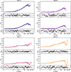 |
Fig. 3. PFS and first harmonic amplitude (A1; data points) for Obs A-D: dashed lines represent the best fit continuum, solid line the best fit model (continuum + gaussian in absorption/emission) and residuals (black points). |
2.3.1. Phenomenological fit of the pulsed fraction spectra
We performed a phenomenological fit of the PFS of the four observations searching for hints of local features in the iron line region (6 − 7 keV) and in the 30 − 40 keV range, where the energy-phase matrix showed sharp variability among the profiles, indicating the possible presence of a CRSF. In addition to the pulsed fraction spectra, we extended our analysis to include the normalised amplitude of the first harmonic, A1, in line with the findings of FDA23.
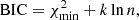
Inspection of the four PFSs shown in Fig. 3 reveals that Obs D exhibits a clear dip in the 30 − 40 keV range. In contrast, this complexity is much less pronounced in the other three observations, for which we nevertheless conducted a dedicated search for similar features. All fits required dividing the data into two distinct energy regions, with Esplit lying in the 9 − 11 keV range (see FDA23 for details), hereafter referred to as the low-energy and high-energy intervals. For each interval, we tested both a simple model consisting of a polynomial continuum and a more complex model that included an additional Gaussian component. We emphasise that the polynomial is used purely for descriptive purposes, without assuming any specific physical model. Its flexibility provides an empirical representation of the PFS continuum, allowing the identification of local deviations potentially associated with spectral features. To avoid overfitting, we selected the best fit model as the one which minimises the Bayesian information criterion (BIC; Schwarz 1978), which under the assumption of Gaussian errors, can be written as
 (2)
(2)
where k,n are the number of free parameters in the model and in the data, respectively. Table 2 shows the differences in the BIC values as Δ (BIC) = BICworst − BICbest.
Best-fit parameters of the Gaussian feature detected at high energies for the PFS and its first harmonic (A1).
Synthesizing the model results, we find that:
-
The PFSA requires a complex model that significantly improves the fit (ΔBIC = −23.3), with a Gaussian at Egau ≈ 34.9 keV (σ ≈ 2.8 keV).
-
For PFSB, limited to E ≲ 35 keV, the data are simply well fitted with a polynomial.
-
The PFSC needs a negative Gaussian at 6.6 keV; at higher energies, residuals are mitigated by a positive Gaussian at ∼23 keV, although its parameters are unconstrained. The PFSC first harmonic instead requires a negative Gaussian at ∼34 keV.
-
The last observation, PFSD, shows the most significant features: both PFSD and its first harmonic increase with energy, but exhibit sharp Gaussian-like drops at low energy (EFe = 6.67 ± 0.06 keV, σFe = 0.53 ± 0.14) and at high energy (Egau = 35.2 ± 0.3 keV,
 , depth ≈ − 1.2; see Table 2).
2.4. Spectral analysis
2.4.1. Methods
In the following, we test the hypothesis that the sharp variability observed near 35 keV, evident in the pulse profiles (Fig. 2), pulsed fraction spectra, and the normalised amplitude of the first harmonic (Fig. 3), originates from a cyclotron resonance. We performed spectral analysis in the restricted energy range 15 − 50 keV, where the continuum can be well approximated by an exponentially cutoff power-law (A(E) = KE−Γexp(−E/Ecut), CUTOFFPL in Xspec), thus minimising the spectral correlations and difficulties involved in the choice of a more complicated broad-band continuum. We used the widely adopted X-ray fitting package Xspec (Arnaud 1996), interfaced via its Python wrapper PyXspec. We compared the fit results of this simple model with those obtained with the same model convolved with a Gaussian absorption feature:
(i) Model1 = CONST × (CUTOFFPL);
(ii) Model2 = CONST × (CUTOFFPL*GABS).
To go beyond the standard frequentist statistic, we employed a Bayesian statistical framework to perform model selection and rigorously assess model uncertainties. For this purpose, we used the BXA package (Bayesian X-ray Analysis; Buchner et al. 2014), which connects Xspec with the UltraNest nested sampling algorithm (Buchner 2021), allowing efficient computation of the posterior distributions. Moreover, it computes the marginal evidence of each model, that is, the likelihood integrated over the prior space
 (3)
(3)
where ℒ(θ) and π(θ) are the likelihood and the prior distribution, respectively. We then identified the preferred model as the one with the highest marginal evidence and quantified the relative support provided by the data through the Bayes factor
 (4)
(4)
where Zbest is the evidence of the best-performing model, while Zmodel is the evidence of the other model. Expressing the Bayes factor in logarithmic form, as log10(BF), we adopted the Jeffreys scale (Jeffreys 1957) to interpret its magnitude, considering log10(BF)≥1 as strong evidence and log10(BF)≥2 as decisive evidence in favour of the model with the larger marginal evidence.
2.4.2. Results
We re-binned the spectra using a Python implementation5 algorithm for optimal binning, following the prescriptions of Kaastra & Bleeker (2016). We adopted uninformative yet physically motivated priors for the parameters of the GABS component, applying a single set of broad priors, motivated by the timing analysis results, across all observations. Specifically, the prior intervals for GABS were: Ecyc = [28.0, 38.0] keV, σ = [0.1, 7.0] keV, and Depth = [0.01, 7.0], as reported in Table 3 along with their corresponding probability distributions. We assumed uniform distributions for all parameters, except for the CUTOFFPL normalisation and the depth of the Gaussian, for which we adopted log-uniform distributions.
Set of priors adopted for the phase-averaged spectral analysis with both Model 1 and Model 2.
For all observations, the model that provides the best description includes the GABS component, even if for Obs A the simple model is only one order of magnitude less probable. The Bayes factors are log10BF = 0.98, 5.1, 25.0, and 23.1 for Obs A, B, C, and D, respectively, indicating decisive support for the presence of the line in Obs B, C, and D and indication for it in Obs A. Figure 4 shows the phase-averaged spectra and residuals for the best fit, while posterior distributions can be found in the online material related to this paper6. For comparison, we also show the residual after setting the depth of the line to zero.
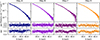 |
Fig. 4. Upper panels: data and best-fitting model (Model2) for the phase averaged-spectra of the four NuSTAR observations. Middle panels: residuals of best-fitting model. Lower panels: residuals of the best-fitting model with a line depth set to zero. |
2.5. Pulse profiles variability at Ecyc
At this stage, a phase-resolved spectral analysis would have been useful to investigate the spectral variability along the spin phase and to relate it to the behaviour of the PFS. However, as the S/N is already low in the phase-averaged spectra above 30 keV, we opted to obtain guidance from pulse-profile variability. The MWCC (Fig. 2) shows that local profile changes emerge at ∼28 keV; we therefore used the 28–31 keV profile (PP28 − 31) as a reference to compute cross-correlation coefficients and phase lags for all profiles above 31 keV. Panels a in Figs. 5 and 6 show PP28 − 31 and their cross-correlations (panel b), colour coded by correlation value; panel b of Fig. 6 also includes the phase lags. Panels c–e present average profiles over energy intervals grouped according to the cross-correlation, using the same colour coding as panel b. Dashed and solid green lines mark the centroids of Ecyc and Egau, PFS, respectively. These complementary techniques reveal sharp profile variability between 30 and 35 keV, particularly prominent at low luminosities. We are led to interpret such abrupt morphological changes as due to the CRSF, where the energy-dependent cross-section has strong resonances that might reflect in the beam pattern and origin of strong variations of the pulse-profile shape.
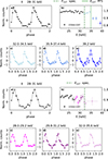 |
Fig. 5. Pulse variability around the cyclotron line for Obs A (top, blue tones) and B (bottom, purple tones). Panel (a): PP28 − 31 (see Sect. 2.5). Panel (b): cross-correlation spectra of the PPs > 20 keV relative to PP28 − 31. Cyclotron energy from the spectral and PFS fits, dashed and solid vertical lines, respectively. Panels (c)–(e): PPs in three energy ranges with consistent cross-correlation values, using the same colour code adopted in panel (b). |
 |
Fig. 6. As in Fig. 5 but for Obs C (top) and D (bottom), including the phase lag spectrum in panel (b). |
3. Discussion
In this paper, we analysed for the first time the PFS, and the energy-resolved PPs, along the outburst of a BeXRB, 4U 1901+03 adopting the same methodology of Ferrigno et al. (2023). We also applied Bayesian spectral analysis to search for the line in the phase averaged spectra motivated by the PPs and PFS results.
The sharp variability of the PPs around 30 keV (see Fig. 2) can be interpreted as the direct manifestation of the CRSF: cyclotron resonance introduces a sudden increase in resonant photon–electron scattering cross-section, which depends on the photon propagation angle relative to the magnetic field. This angular dependence redistributes photons at the resonance energy, modifying the observed PPs. In fact, this relationship has been confirmed by observations (see Ferrigno et al. 2011, FDA23) and is also grounded in theoretical and computational studies (Schönherr et al. 2014). In addition, recent developments on modelling have been able to qualitatively reproduce the observed PPs, and the effects of spin phase spectral variability on the PFS at the CRSF energy (D’Aì et al. 2025; Maniadakis et al. 2025).
Focusing on the general trend of the PFS, we note that it is closely related to the source flux. Obs A and B have similar fluxes and a very similar PFS energy dependence. The PFS of Obs C, however, displays a bump at a lower energy than Ecycl derived from spectral analysis, a feature also reported in Maniadakis et al. (2025) for 4U 1538–52. Conversely, the PFS of Obs D is similar to those analysed by Ferrigno et al. (2023), showing a rising trend with energy and a well-defined Gaussian-like dip (see Table 2 and Fig. 3). Following Maniadakis et al. (2025), the presence of a dip or a bump in the PFS depends on the phase-dependent variation of the CRSF. Therefore, the distinct PFS behaviour observed suggests a change in the beam pattern as a function of luminosity. A similar flux-dependent trend of the PFS of 4U 1901+03 was reported by Chen et al. (2008) for the 2003 outburst; specifically, the middle panel of their Fig. 4 displays a PFS, at a flux comparable to Obs C, with a flat trend in the 10–20 keV range followed by a bump, which matches our findings. This comparison supports the interpretation that the observed behaviour is intrinsic to the source’s emission mechanism at specific luminosity regimes.
We find evidence for a Gaussian-like absorption feature at ≈32 keV in all four observations (Table 4), with strong to decisive support in three cases (B, C, and D) and moderate evidence in the remaining one (A). The centroid energy does not vary significantly, ≈1.6%, despite a factor of three change in luminosity, while the line depth is luminosity dependent. Our results are partially in contrast with those of Beri et al. (2021), who detected the line in the phase-averaged spectra only for low-luminosity observations, and only in specific phase-resolved intervals for high-luminosity states. Nabizadeh et al. (2021) reported the line in all phase-averaged spectra; while their results for the two low-luminosity observations agree with ours, they found higher centroid energies (Ecyc, ≈39 and 35 keV) and widths (σ ≈ 10 and 9.9 keV) for Obs A and B, respectively. In their analysis, the centroid energy appears to vary with luminosity. In contrast, in our study Ecyc centroid remains consistent within the uncertainties in all four observations. Although a luminosity-dependent variation of the line, as observed in other sources, cannot be excluded, the limited statistics above 40 keV prevented us from testing this scenario further. A shallow dip in the energy spectrum can be observed at the intersection of two continuum components during low-luminosity states (LX < 1035 erg s−1), as previously reported for several sources (e.g. Malacaria et al. 2026, and references therein). However, theoretical simulations demonstrate that resonant scattering induces a sharp angular redistribution of photons, forcing them to escape preferentially perpendicular to the magnetic field lines at the CRSF energy (see, e.g. Schönherr et al. 2014). This mechanism results in significant energy-dependent variability in the pulse profiles. Consistent with these findings, our timing analysis revealed sharp, narrow-range features in both the cross-correlation and PFS. These features were observed at approximately the same energy, regardless of the varying luminosity levels or changes in the underlying spectral shape.
Posterior parameter estimates for the cyclotron resonance model.
A weak luminosity dependence of the cyclotron line energy might be possible when a source is observed close to the critical luminosity, where the accretion flow transitions between sub- and super-critical regimes and the emission geometry changes from a pencil- to a fan-beam configuration (Becker et al. 2012; Mushtukov et al. 2015). This behaviour has been observed in systems like V 0332+53 and A 0535+262, where Ecyc remains approximately constant over a limited luminosity range around the transition (Tsygankov et al. 2010; Kong et al. 2021). However, while the energy remains consistent within uncertainties, we observe an anti-correlation between the line optical depth and luminosity: the line is shallower at the outburst peak and deepens as the luminosity declines. This behaviour can be explained by invoking the transition from a radiation-pressure-dominated flow, where multiple resonant scatterings in a dense column result in a ‘fill in’ of the absorption feature (Nishimura 2014), to a lower-luminosity state that produces a cleaner, more pronounced line profile. A similar conclusion was also reached by Tuo et al. (2020), based on Insight-HMXT observations taken outside the outburst peak, although through different arguments.
For an observed cyclotron line energy of Ecycl ≈ 32 keV, the surface magnetic field is estimated to be B12 ∈ [3.3, 3.9]7. This corresponds to a critical luminosity of  erg s−1. Given the lack of consensus on the distance to 4U 1901+03, we adopted a conservative range of 7 − 12.5 kpc to estimate a luminosity range8. Within this interval, the luminosity ranges (for fluxes reported in Table 1) are : LA ∈ [4.1, 13.0], LB ∈ [4.7, 15.0], LC ∈ [2.6, 8.4], and LD ∈ [1.6, 5.1] (in 1037 erg s−1 units). Within a distance of d ≈ 10 kpc, Obs C would be in the range of critical luminosity for the estimated magnetic field.
4. Conclusions
In this paper, we have shown how a synergic view of timing and spectral features aligns to build a coherent picture of the presence of the CRSF in this source. We have exploited timing and spectral analyses in a complementary manner, showing that the pulsed profiles display a persistent, energy-localised variation that is consistently observed across the four observations through a moving cross-correlation analysis. This behaviour represents a robust, model-independent signature of the imprint of the cyclotron resonant scattering feature on the pulse profiles. By using timing information to identify departures from a simple power-law continuum at the corresponding energies, we suggest that the source is close to the critical luminosity undergoing a transition, evidenced by changes in the width and depth of the cyclotron scattering feature.
Data availability
The data used in this work can be found in the related online repository: https://zenodo.org/records/19068400.
Acknowledgments
E.A. thanks Melania Del Santo, Domitilla De Martino and Valentina La Parola for insightful discussions and thoughtful comments that helped improve this work. The Authors thank the referee for their very constructive report. EA acknowledges support from the INAF MINI-GRANTS number 1.05.23.04.04 for the project PPANDA (Pulse Profiles of Accreting Neutron Stars Deeply Analysed). This research was supported by the International Space Science Institute (ISSI) in Bern, through the ISSI Working Group project Disentangling Pulse Profiles of (Accreting) Neutron Stars.. EA, AD, GC acknowledge funding from the Italian Space Agency, contract ASI/INAF n.I/004/11/4. AD and FP acknowledge support from SEAWIND grant funded by the European Union – Next Generation EU, Mission 4 Component 1 CUP C53D23001330006. FP and AD acknowledge the INAF GO/GTO grant number 1.05.23.05.12 for the project OBIWAN (Observing high B-fIeld Whispers from Accreting Neutron stars). G.V. acknowledges support from the Hellenic Foundation for Research and Innovation (H.F.R.I.) through the project ASTRAPE (Project ID 7802) A.T. acknowledges supercomputing resources and support from ICSC – Centro Nazionale di Ricerca in High Performance Computing, Big Data and Quantum Computing – and hosting entity, funded by European Union – NextGenerationEU. E.S.L. acknowledges support from the FAU Emerging Talents Initiative and funding from the European Union’s Horizon 2020 programme under the AHEAD2020 project (grant agreement No. 871158). We made use of Heasoft and NASA archives for the NuSTAR data. We developed our own timing code for the epoch folding, orbital correction, building of time-phase and energy-phase matrices. This code is based partly on available Python packages such as: Astropy (Astropy Collaboration 2013, 2018, 2022), lmfit (Newville et al. 2014), matplotlib (Hunter 2007), emcee (Foreman-Mackey et al. 2013), stingray (Huppenkothen et al. 2019; Bachetti et al. 2024), corner (Foreman-Mackey 2016), scipy (Virtanen et al. 2020).
References
- Alonso-Hernández, J., Fürst, F., Kretschmar, P., Caballero, I., & Joyce, A. M. 2022, A&A, 662, A62 [NASA ADS] [CrossRef] [EDP Sciences] [Google Scholar]
- Arnaud, K. A. 1996, ASP Conf. Ser., 101, 17 [Google Scholar]
- Astropy Collaboration (Robitaille, T. P., et al.) 2013, A&A, 558, A33 [NASA ADS] [CrossRef] [EDP Sciences] [Google Scholar]
- Astropy Collaboration (Price-Whelan, A. M., et al.) 2018, AJ, 156, 123 [Google Scholar]
- Astropy Collaboration (Price-Whelan, A. M., et al.) 2022, ApJ, 935, 167 [NASA ADS] [CrossRef] [Google Scholar]
- Bachetti, M., Huppenkothen, D., Stevens, A., et al. 2024, J. Open Source Softw., 9, 7389 [Google Scholar]
- Basko, M. M., & Sunyaev, R. A. 1976, MNRAS, 175, 395 [Google Scholar]
- Becker, P. A., & Wolff, M. T. 2022, ApJ, 939, 67 [NASA ADS] [CrossRef] [Google Scholar]
- Becker, P. A., Klochkov, D., Schönherr, G., et al. 2012, A&A, 544, A123 [NASA ADS] [CrossRef] [EDP Sciences] [Google Scholar]
- Beri, A., Girdhar, T., Iyer, N. K., & Maitra, C. 2021, MNRAS, 500, 1350 [Google Scholar]
- Buchner, J. 2021, J. Open Source Softw., 6, 3001 [CrossRef] [Google Scholar]
- Buchner, J., Georgakakis, A., Nandra, K., et al. 2014, A&A, 564, A125 [NASA ADS] [CrossRef] [EDP Sciences] [Google Scholar]
- Chen, W., Qu, J.-L., Zhang, S., Zhang, F., & Zhang, G.-B. 2008, Chin. Astron. Astrophys., 32, 241 [Google Scholar]
- D’Aì, A., Maniadakis, D. K., Ferrigno, C., et al. 2025, A&A, 694, A316 [NASA ADS] [CrossRef] [EDP Sciences] [Google Scholar]
- Ferrigno, C., Falanga, M., Bozzo, E., et al. 2011, A&A, 532, A76 [CrossRef] [EDP Sciences] [Google Scholar]
- Ferrigno, C., D’Aì, A., & Ambrosi, E. 2023, A&A, 677, A103 [NASA ADS] [CrossRef] [EDP Sciences] [Google Scholar]
- Foreman-Mackey, D. 2016, J. Open Source Softw., 1, 24 [Google Scholar]
- Foreman-Mackey, D., Hogg, D. W., Lang, D., & Goodman, J. 2013, PASP, 125, 306 [Google Scholar]
- Forman, W., Jones, C., & Tananbaum, H. 1976, ApJ, 206, L29 [NASA ADS] [CrossRef] [Google Scholar]
- Galloway, D. K., Wang, Z., & Morgan, E. H. 2005, ApJ, 635, 1217 [NASA ADS] [CrossRef] [Google Scholar]
- Hunter, J. D. 2007, Comput. Sci. Eng., 9, 90 [NASA ADS] [CrossRef] [Google Scholar]
- Huppenkothen, D., Bachetti, M., Stevens, A. L., et al. 2019, ApJ, 881, 39 [Google Scholar]
- Jeffreys, H. 1957, MNRAS, 117, 347 [Google Scholar]
- Kaastra, J. S., & Bleeker, J. A. M. 2016, A&A, 587, A151 [NASA ADS] [CrossRef] [EDP Sciences] [Google Scholar]
- Kong, L. D., Zhang, S., Ji, L., et al. 2021, ApJ, 917, L38 [NASA ADS] [CrossRef] [Google Scholar]
- Krimm, H. A., Holland, S. T., Corbet, R. H. D., et al. 2013, ApJS, 209, 14 [NASA ADS] [CrossRef] [Google Scholar]
- Malacaria, C., Jenke, P., Roberts, O. J., et al. 2020, ApJ, 896, 90 [NASA ADS] [CrossRef] [Google Scholar]
- Malacaria, C., Pike, S. N., D’Aì, A., et al. 2026, A&A, 706, A321 [NASA ADS] [CrossRef] [EDP Sciences] [Google Scholar]
- Maniadakis, D. K., Sokolova-Lapa, E., D’Aì, A., et al. 2025, A&A, 700, A70 [NASA ADS] [CrossRef] [EDP Sciences] [Google Scholar]
- Mushtukov, A., & Tsygankov, S. 2022, ArXiv e-prints [arXiv:2204.14185] [Google Scholar]
- Mushtukov, A. A., Suleimanov, V. F., Tsygankov, S. S., & Poutanen, J. 2015, MNRAS, 447, 1847 [NASA ADS] [CrossRef] [Google Scholar]
- Nabizadeh, A., Tsygankov, S. S., Ji, L., et al. 2021, A&A, 652, A89 [NASA ADS] [CrossRef] [EDP Sciences] [Google Scholar]
- Newville, M., Stensitzki, T., Allen, D. B., & Ingargiola, A. 2014, https://doi.org/10.5281/zenodo.11813 [Google Scholar]
- Nishimura, O. 2014, ApJ, 781, 30 [NASA ADS] [CrossRef] [Google Scholar]
- Reig, P. 2011, Ap&SS, 332, 1 [Google Scholar]
- Schönherr, G., Schwarm, F.-W., Falkner, S., et al. 2014, A&A, 564, L8 [NASA ADS] [CrossRef] [EDP Sciences] [Google Scholar]
- Schwarm, F. W., Ballhausen, R., Falkner, S., et al. 2017, A&A, 601, A99 [NASA ADS] [CrossRef] [EDP Sciences] [Google Scholar]
- Schwarz, G. E. 1978, Ann. Stat., 6, 461 [CrossRef] [Google Scholar]
- Sokolova-Lapa, E., Stierhof, J., Dauser, T., & Wilms, J. 2023, A&A, 674, L2 [NASA ADS] [CrossRef] [EDP Sciences] [Google Scholar]
- Staubert, R., Trümper, J., Kendziorra, E., et al. 2019, A&A, 622, A61 [NASA ADS] [CrossRef] [EDP Sciences] [Google Scholar]
- Stierhof, J. J. R., Sokolova-Lapa, E., Berger, K., et al. 2025, A&A, 698, A308 [NASA ADS] [CrossRef] [EDP Sciences] [Google Scholar]
- Tsygankov, S. S., Lutovinov, A. A., & Serber, A. V. 2010, MNRAS, 401, 1628 [NASA ADS] [CrossRef] [Google Scholar]
- Tuo, Y. L., Ji, L., Tsygankov, S. S., et al. 2020, J. High Energy Astrophys., 27, 38 [NASA ADS] [CrossRef] [Google Scholar]
- Virtanen, P., Gommers, R., Oliphant, T. E., et al. 2020, Nat. Methods, 17, 261 [Google Scholar]
Swift/BAT transient monitor results provided by the Swift/BAT team (Krimm et al. 2013).
Provided by the Fermi-GBM pulsar database: https://https://gammaray.nsstc.nasa.gov/gbm/science/pulsars.html Malacaria et al. (2020).
See FDA for an extensive analysis of the different definitions of the pulsed fraction.
See https://gitlab.astro.unige.ch/ferrigno/optimal-binning
B12 = (1 + z)×Ecycl(keV)/11.57, assuming a gravitational redshift z ∈ [1.2, 1.4] for typical neutron star parameters.
Distance estimates vary significantly: Gaia EDR3 suggests 4.5 − 5.6 kpc, though the parallax is poorly constrained (ϖ ≈ 0.0005 ± 0.2 mas). While Tuo et al. (2020) proposed ≈12.4 kpc via torque modelling, Stierhof et al. (2025) argue that current analytic torque models are subject to significant systematics and may not yet allow for reliable quantitative measurements of the magnetic field or associated parameters. We thus treat the torque-derived value only as a tentative upper limit. Conversely, the high source extinction (E(B − V)≈2.5 − 3.5) favours a distance of at least ≈7 kpc, where Galactic dust maps (e.g. Bayestar2019) typically saturate.
All Tables
Best-fit parameters of the Gaussian feature detected at high energies for the PFS and its first harmonic (A1).
Set of priors adopted for the phase-averaged spectral analysis with both Model 1 and Model 2.
All Figures
|
Fig. 1. Swift/BAT light curve of the 2019 giant outburst (15–50 keV), rate in count s−1 cm−2; vertical lines mark the epochs of the four NuSTAR observations. |
| In the text | |
|
Fig. 2. Energy-phase maps and MWCC with a window of two adjacent bins (see text). For each panel, we chose Nbins = 20 and S/N = 5.0. The colour bar, on the right side of each map, represents the values of the normalised profiles plotted in the map and spans between the minimum and the maximum of the entire map. |
| In the text | |
|
Fig. 3. PFS and first harmonic amplitude (A1; data points) for Obs A-D: dashed lines represent the best fit continuum, solid line the best fit model (continuum + gaussian in absorption/emission) and residuals (black points). |
| In the text | |
|
Fig. 4. Upper panels: data and best-fitting model (Model2) for the phase averaged-spectra of the four NuSTAR observations. Middle panels: residuals of best-fitting model. Lower panels: residuals of the best-fitting model with a line depth set to zero. |
| In the text | |
|
Fig. 5. Pulse variability around the cyclotron line for Obs A (top, blue tones) and B (bottom, purple tones). Panel (a): PP28 − 31 (see Sect. 2.5). Panel (b): cross-correlation spectra of the PPs > 20 keV relative to PP28 − 31. Cyclotron energy from the spectral and PFS fits, dashed and solid vertical lines, respectively. Panels (c)–(e): PPs in three energy ranges with consistent cross-correlation values, using the same colour code adopted in panel (b). |
| In the text | |
|
Fig. 6. As in Fig. 5 but for Obs C (top) and D (bottom), including the phase lag spectrum in panel (b). |
| In the text | |
Current usage metrics show cumulative count of Article Views (full-text article views including HTML views, PDF and ePub downloads, according to the available data) and Abstracts Views on Vision4Press platform.
Data correspond to usage on the plateform after 2015. The current usage metrics is available 48-96 hours after online publication and is updated daily on week days.
Initial download of the metrics may take a while.