| Issue |
A&A
Volume 709, May 2026
|
|
|---|---|---|
| Article Number | A161 | |
| Number of page(s) | 9 | |
| Section | Extragalactic astronomy | |
| DOI | https://doi.org/10.1051/0004-6361/202557957 | |
| Published online | 13 May 2026 | |
The shortest detected intra-day variability of active galactic nuclei in the TESS survey
Homer L. Dodge Department of Physics and Astronomy, University of Oklahoma, 440 W. Brooks St., Norman, OK 73019, USA
★ Corresponding author: This email address is being protected from spambots. You need JavaScript enabled to view it.
Received:
3
November
2025
Accepted:
23
March
2026
Abstract
Context. Active galactic nuclei (AGNs) are known to be variable in almost all wavelengths and timescales. The shortest AGN variability timescale can be used to probe the smallest scale structures within AGNs.
Aims. We aim to measure the shortest detected variability timescale, tmin, ul, of type 1 radio-quiet Seyfert galaxies and to analyse their characteristics.
Methods. We extracted the Transiting Exoplanet Survey Satellite (TESS) light curves of 47 Seyfert 1 galaxies. We measured the power spectral densities (PSDs) of the sample, modelled by a power law model plus constant noise. We constrained the shortest detected AGN variability timescale, whereby the power law component exceeds the constant noise and systematic uncertainties indicated by the upper limits of non-variable quiescent galaxies’ PSDs.
Results. We measured the upper limits of the shortest variability timescale to be log(tmin, ul/h) = 0.85 ± 0.55. We compared these upper limits to a range of theoretical AGN variability timescales and the natural interpretation of our measured tmin, ul is the light-crossing scale from a coherently varying region, where the measured tmin, ul corresponds to the range from a few to thousands of gravitational radii. A significant fraction of these light-crossing scales is smaller than the accretion disc emission sizes measured by quasar microlensing, reverberation mapping, or theoretical accretion disc models. Since we only measured the upper limits, the true physical shortest variability timescales are even shorter. We measure the power law index as α = 2.0 ± 0.2 and we found weak anti-correlations with the black hole mass and luminosity.
Conclusions. Our analysis suggests that the shortest optical variability is driven by a compact region that is smaller than the accretion disc size, potentially as a result of X-ray reprocessing. Alternatively, this shortest timescale variability suggests that the accretion disc can be inhomogeneous. This could potentially be caused by turbulence from magnetorotational instability or magnetic reconnections.
Key words: galaxies: active / galaxies: Seyfert
© The Authors 2026
 Open Access article, published by EDP Sciences, under the terms of the Creative Commons Attribution License (https://creativecommons.org/licenses/by/4.0), which permits unrestricted use, distribution, and reproduction in any medium, provided the original work is properly cited.
This article is published in open access under the Subscribe to Open model. This email address is being protected from spambots. You need JavaScript enabled to view it. to support open access publication.
1. Introduction
Active galactic nuclei (AGNs) are observed to be variable throughout the entire electromagnetic spectrum on almost all timescales. Overall, AGN variability provides useful insights about the inner structures of AGNs. One example is the light-crossing scale. As light travels at a finite speed, the variability timescale can be scaled by the speed of light to measure the size of the coherently varying region emitting at that wavelength. For example, AGN variability was first observed on timescale of several days, suggesting that the size of an AGN is of the order of the Solar System. This led to the idea of AGN being powered by accretion of material onto a compact object: namely, a supermassive black hole (SMBH; Lynden-Bell 1969). The light-crossing scale has been routinely applied to different wavelengths to constrain AGN emission sizes to the first order in the optical, infrared (IR), and X-ray bands (e.g. Fabian et al. 2015; Pozo Nuñez et al. 2015; Jha et al. 2022). Another example is reverberation mapping, by measuring the time lag between brightness fluctuations in different wavelengths, which corresponds to different regions in the AGN structure, observers can estimate the size of the broad line region (BLR) of the AGN and the mass of the SMBH (e.g. Peterson 1993). Studying the power spectral densities (PSDs) of AGNs also provides an alternative method to probe the SMBH. AGN PSDs are often modelled with a broken power law and the break frequency (i.e. the location where the power law index shifts) is observed to be correlated with the black hole mass (e.g. Kelly et al. 2009; MacLeod et al. 2010; González-Martín 2018; Burke et al. 2021; Tarrant et al. 2025).
Variability observed on timescales shorter than a day, or intra-day, intra-night, or micro-variability, is important in AGN studies, as it can be used to probe the smallest structures of AGNs. The SMBH or its innermost stable orbit might provide the shortest timescale, but if variability arises from accretion disc inhomogeneities, the observed variability timescale can be even smaller. Potentially, there can be no lower limit on the variability timescale and, thus, the measurement of shortest AGN variability timescale can provide an important insight into the source of AGN variability.
The short timescale in AGN variability in X-rays is well studied because of the larger AGN variability amplitudes in this band and the photon counting nature of X-ray observations. X-ray AGN PSD studies have reported that variability is detected in frequencies upwards of 10−4 Hz to 10−2 Hz or on timescales of minutes to hours (e.g. Uttley et al. 2002; Markowitz et al. 2003; McHardy et al. 2004; González-Martín & Vaughan 2012; González-Martín 2018; Rani et al. 2025). This would suggest that the X-ray emitting region is of the order of a few rg, which is consistent with independent measurements from microlensing (e.g. Morgan et al. 2008; Dai et al. 2010).
Optical AGN variability studies are often limited by the fact that the data primarily come from ground-based telescopes, combined with the smaller intra-day variability amplitudes, and as a result, high-cadence monitoring data of AGN is rare and measurements of intra-day variability can be challenging. Many previous intra-day optical AGN variability involved using statistical methods, such as an F-test, to detect variability, along with measuring the variability amplitude and the duty cycle, which is the fraction of time when the AGN is shown to be varying (e.g. Romero et al. 1999; Goyal et al. 2012, 2013; Kumar et al. 2015; Ojha et al. 2019). Different classes of AGNs display different duty cycles (i.e. greater duty cycles were reported for AGNs with higher radio loudness and optical polarization) suggesting different physical conditions (e.g. Romero et al. 1999; Goyal et al. 2013). Also, many of these studies were conducted on blazars or radio-loud AGNs, where the variability is strongly affected by the relativistic jet, which makes them less ideal for understanding the innermost structure of AGNs.
The advent of high-cadence long-term space-based timing surveys opened a new window for intra-day optical AGN variability studies. The Kepler Space Telescope, making observations with a cadence of the order of minutes over many years, enabled optical PSD studies similar to X-ray studies (e.g. Aranzana et al. 2018; Smith et al. 2018), where the variability of timescales (i.e. hours to days) was detected. Transiting Exoplanet Survey Satellite (TESS; Ricker et al. 2015) is another space-based high-cadence survey mission. While Kepler is limited to a specific region in the celestial sphere, covering approximately 116 square degrees, TESS is an all-sky survey, providing the ideal data set for the variability study of a general AGN population. Recent intra-day AGN variability studies using the TESS data involve blazars and radio-loud AGNs (e.g. Dingler & Smith 2024; Yang et al. 2024). To study the short-timescale optical variability near the central engine, we focus on examining TESS light curves of radio-quiet AGNs.
In this study, we seek to measure the upper limits of the shortest AGN variability timescale, tmin, ul, that is detectable in the TESS survey. As mentioned earlier, observations reveal that the AGN PSDs are modelled by a single or broken power law (e.g. McHardy et al. 2004; González-Martín 2018). By measuring the frequency where the power law component dominates over noise or systematics, we can measure the shortest detected variability timescale. We introduce our sample and data in Section 2 and describe methods in Section 3. We present our results in Section 4, discuss the implications of these results in Section 5, and present our conclusions in Section 6. Throughout this paper, we assume the ΛCDM cosmological model with ΩΛ = 0.7, ΩM = 0.3, and H0 = 70 km s−1 Mpc−1.
2. Sample and data
We examined a sample of bright Seyfert galaxies with at least one TESS sector observed. Our sample is primarily derived from the AGN sample of González-Martín (2018) and the Swift BAT 9-month AGN catalogue (Tueller et al. 2008). We limited our sample to type 1, as type 2 Seyfert galaxies are observed to display very weak to non-detectable TESS variability (e.g. Kovacevic et al. 2025). We followed the classification of the respective catalogue. To exclude radio-loud AGNs, we used the radio loudness parameter, ℛ = F5 GHz/FB, where F5 GHz and FB are flux density in the 5 GHz and B bands, respectively. AGNs with ℛ > 10 are classified as radio-loud AGNs (e.g. Chiaberge & Marconi 2011). We retrieved photometry information from NASA/IPAC Extragalactic Database (NED)1. The final sample size is 47 and they are listed on Table A.1.
For this sample, we also gathered the black hole mass from literature. The black hole masses reported by Koss et al. (2017) using the single-epoch Hβ emission do not include uncertainties. Instead, the authors noted that this method is known to have systematic uncertainties of about 0.3 dex, which we used as the uncertainties in this work. The black hole masses were not reported for a few objects. For these objects, we retrieved the V-band magnitudes of these targets from All-Sky Automated Survey for SuperNovae (ASAS-SN; Shappee et al. 2014a; Kochanek et al. 2017), estimated the I-band spheroid luminosity, and employed the spheroid luminosity scaling relation of Bennert et al. (2021), as described in Yuk et al. (2022).
TESS is a satellite designed to scan a portion of the sky with high cadence, for approximately 27 days at a time. After each 27-day cycle, called a sector, it points at a different position, eventually covering the entire celestial sphere. It is equipped with four cameras, each with 24° by 24° field of view, observing 24° by 96° simultaneously. TESS filter spans from 600 to 1000 nm. The primary mission, which began with launch in 2018 until sector 26 in July 2020, took full-frame images (FFIs) every 30 minutes. Following the primary mission was the first extended mission, which lasted until sector 55 in September 2022 with a 10-minute cadence FFIs. Since then, TESS entered the second extended mission, which is observing with a 200-second cadence. The typical limiting magnitudes are approximately 19.6 for 30-minute FFIs, 19.0 for 10-minute FFIs, and 18.4 for 200-second FFIs. For this study, we limited our data to primary and first extended missions.
We extracted the TESS light curves using the image subtraction method. First, the FFIs were cut into 750 pixel by 750 pixels postage stamps around the target. Then the first 100 good images were combined into a reference image. This reference image was subtracted from all postage stamps. Then we performed point spread function (PSF) photometry on the subtracted images to measure the flux relative to the reference image. More detailed information on the TESS light curve extraction method can be found in Fausnaugh et al. (2021) and Vallely et al. (2021).
Following the extraction of the light curve, we also examined the light curves of nearby pixels for any anomalies that would have been potentially caused by the instrument or a nearby source affecting the galaxy’s light curve. Some examples of anomalies can be found in Yuk & Dai (2025).
We also extracted TESS light curves of quiescent galaxies to measure the systematic variability. These galaxies are selected from the Two-Micron All Sky Survey (2MASS; Skrutskie et al. 2006) extended sources catalogue (Jarrett et al. 2000), which are bright (K < 11.34) and away from the galactic plane (|b|> 15°). In addition, we required the galaxy sample to fall in the magnitude range of the Swift BAT nine-month AGN sample and display comparable average flux uncertainties. In total, we analysed TESS light curves of 17 galaxies to examine the systematics. The galaxies’ flux distribution is log(F/mJy) = 0.96 ± 0.38, while the AGNs’ flux distribution is log(F/mJy) = 1.06 ± 0.43.
3. Methods
TESS light curves were primarily sampled in regular intervals. However, in the middle of a sector, there is a discontinuity of approximately one day for the data transmission. In addition, removing bad data points or outliers can introduce additional gaps. Thus, we used the Lomb-Scargle periodogram (e.g. Lomb 1976; Scargle 1982) to construct the PSDs from TESS light curves, which is ideal for computing the PSDs for unevenly sampled light curves. We computed the PSD within the frequency range of 1/T to 1/(2ΔTsamp), where T is the duration of a sector (∼27 days) and ΔTsamp is the sampling interval (30 minutes for sectors ≤26 and 10 minutes for sectors > 26). We then binned the PSDs by a factor of 1.6, and took the standard deviation of the mean for each bin as the uncertainty. The Lomb-Scargle periodogram method was previously used to successfully measure AGN PSDs using TESS data (e.g. Burke et al. 2021; Yuk & Dai 2025).
Although AGN PSDs are commonly measured as a broken power law, the typical break frequency is of the order of 10−3 to 10−2 day−1 (e.g. Burke et al. 2021; Tarrant et al. 2025; Yuk & Dai 2025), which is below the range of TESS frequencies. Some studies report high-frequency breaks in the TESS PSD regime (e.g. Burke et al. 2020; Yuk & Dai 2025), and these high-frequency breaks are at the low frequency part of the TESS PSDs, which affect little to the measurement of PSDs at high frequencies. We chose to use a simple power law model to fit the TESS PSD to simplify the analysis:
 (1)
(1)
where P is the power, A is the amplitude at νref, νref is the reference frequency (set to the median value of TESS ν range), and C is the white noise level. Once the model is fit, theoretically, the shortest variability timescale can be calculated by computing the frequency where the power law component exceeds the noise, νmax = νref(C/A)−1/α. We tested the broken power law model in the discussion and yielded consistent νmax values.
However, it is possible for systematic variability to be present in the TESS light curves. To examine it, we reduced TESS light curves of several quiescent galaxies, computed the PSDs, and fit the power law plus white noise model. We found α ∼ 1.5 for systematic variability measured in quiescent galaxies and α ∼ 2.0 for AGNs. This suggests that TESS light curves of galaxies can show a red noise spectrum due to systematic effects; however, the slope is shallower than the red noise spectrum of AGNs. Even more importantly, the amplitudes for galaxy spectra are smaller, enabling us to detect AGN variability beyond these noises. In particular, we measured the mean and the standard deviation of the PSD with respect to the white noise level for the quiescent galaxies’ PSDs. We estimated the upper limit of the systematic variability as the mean plus three-sigma of the galaxies’ PSDs. We located where the AGN PSDs exceed this upper limit to measure the shortest variability timescale. An example of comparing galaxies’ average PSD and an AGN PSD is shown on Figure 1. For AGNs with multiple TESS sectors, we computed νmax for each sector separately. We found a scatter in νmax measurements among different sectors, suggesting that sector-to-sector and pixel-to-pixel dependent instrumental factors are present. Due to our sample size constraints, we were unable to characterise these dependences. Thus, for this sub-sample of AGNs, we took the largest νmax as our shortest detected variability timescale, tmin, ul. As the measured tmin, ul values from this method are in the observed frame, we corrected it by a factor of (1 + z) to calculate the rest-frame timescale for further analysis.
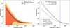 |
Fig. 1. Left: Systematics of TESS survey and light curve extraction technique indicated by the PSDs of non-variable galaxy light curves, where the y-axis is the scaled power relative to the constant white noise. Each gray line indicates the power law plus white noise fit for an individual galaxy’s light curve, the black line represents the mean galaxy PSD, and the red and yellow shaded areas represent the one-sigma and three-sigma limits, respectively. Right: Comparison between Seyfert 1 AGN, ESO 362-G018, Sector 5 PSD (which has the measured tmin, ul value equal to the median of the AGN sample), and the upper limits of galaxies as a representative to illustrate the measurement of the shortest detected variability timescale. The text next to the PSD lists the parameters for the best fit. The PSDs in both panels are normalised by their respective noise levels. |
To complement the timescale measurements, we also computed the structure function. To calculate the structure function, we used the following definition,
![Mathematical equation: $$ \begin{aligned} \mathrm{SF}(\tau ) = \sqrt{\langle [m(t-\tau )-m(t)]^2\rangle -\sigma _{\mathrm{noise}}^2}, \end{aligned} $$](/articles/aa/full_html/2026/05/aa57957-25/aa57957-25-eq2.gif) (2)
(2)
where τ is the time lag between two observations, m is the magnitude, and
 (3)
(3)
is the uncertainty correction where σerr is the measurement uncertainty in magnitude (e.g. Bauer et al. 2009; Middei et al. 2017). The AGN structure functions are measured with an increasing trend at long timescales as expected; however, we found that the power law with white noise model fits poorly to structure functions. So, for each structure function, we estimated the noise level to be the average of the smallest 25% of the structure function, which typically locates at the shortest timescale segment and normalised the structure function by this noise estimate. The normalised structure functions of galaxies and AGNs were then compared to measure tmin, ul (Figure 2).
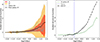 |
Fig. 2. Left: Distribution of quiescent galaxies’ structure functions, normalised by the noise level, similar to Figure 1 left. Right: Comparison of structure functions of galaxies and NGC 931 sector 18 to demonstrate the smallest variability timescale measurement. |
4. Results
Out of the 47 AGNs, we measured the shortest detected variability timescales for 32. We measured the νmax ranges from 1.2 × 10⁻¹ to 3.5 × 101 day−1, with the median at 3.4 day−1. Conversely, the shortest variability timescale detected by TESS light curves ranges from 0.68 to 193 hours, with the median at 7.1 hours, or log(tmin, ul/h) = 0.85 ± 0.55. The distribution of tmin, ul = 1/νmax is shown on Figure 3. We found that the remaining 15 AGNs have low variability amplitudes, with a power law component that is lower than the systematics.
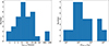 |
Fig. 3. Left: Distribution of the shortest detected TESS variability timescales of the sample. Right: Histogram showing the distribution of ctmin, ul in terms of rg. |
The light-crossing scale is the most natural explanation for these short-timescale variations. In Figure 4, we compare the light-crossing scale corresponding to the shortest variability timescale to the gravitational radius of the black holes, rg = GM/c2, the quasar microlensing accretion disc size measurements, and the theoretical and measured accretion disc scaling relations with black hole mass. These light-crossing scales correspond to a range from a few to thousands of rg, while for massive black holes, we can probe the variability down to a few rg (Figure 4). The quasar microlensing accretion disc size of Morgan et al. (2010) is
 (4)
(4)
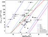 |
Fig. 4. Distribution of the shortest detected TESS variability timescales of the sample, plotted against the black hole mass. The blue dashed lines indicate the different values of gravitational radii for the given black hole mass, and the green and red solid lines indicate the theoretical and measured accretion disc and corona sizes from literature (Shakura & Sunyaev 1973; Morgan et al. 2010; Dogruel et al. 2020). |
While Morgan et al. (2010) measured disc size in the rest-frame UV, we chose to scale the size to the TESS band via R ∝ λ4/3. The X-ray emitting region size for radio-quiet quasars by Dogruel et al. (2020) is
 (5)
(5)
The thin-disc theoretical model prediction is:
 (6)
(6)
where λrest is the rest wavelength, L/LE is the Eddington ratio, and η is the accretion efficiency (e.g. Shakura & Sunyaev 1973; Morgan et al. 2010). As our sample is made up of local bright Seyfert galaxies with low redshifts, we approximated λrest as the central wavelength of TESS (∼780 nm), the Eddington ratio as L/LE = 0.3, and the accretion efficiency as η = 0.1.
Out of 32 AGNs with tmin, ul measurements, we found that for 17 AGNs, the ctmin, ul values are consistent or above the accretion disc size from the thin disc model by Shakura & Sunyaev (1973), 15 are consistent or above the microlensing accretion disc size measurement of Morgan et al. (2010), and all of them are greater; however, only one is consistent with the microlensing measurement of X-ray emitting region size by Dogruel et al. (2020). Finally, 47% to 53% of the sample display variability in scales smaller than the size of the accretion disc in optical wavelength from thin disc prediction or microlensing measurements, respectively. This suggests that the source of the optical variability is smaller in size, some approaching the size of the X-ray corona.
We measured the power law indices to be α = 2.0 ± 0.2. This is consistent with the damped random walk model (DRW; (e.g. Kelly et al. 2009; Kozłowski 2016) at the high frequency regime. We note that Kepler PSD studies, which probe similar timescales, report steeper high-frequency power law index measurements (e.g. Mushotzky et al. 2011; Smith et al. 2018), which requires further investigation for confirmation. We discovered that the power-law index is weakly correlated with pseudo-Eddington ratio (r = 0.38, p = 0.03), weakly anti-correlated with the black hole mass (r = −0.33, p = 0.07), and uncorrelated with luminosity (r = −0.23, p = 0.21) (Figure 5). The significance of these weakly correlated relations is low and a larger sample is needed to further confirm these correlations.
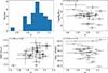 |
Fig. 5. Top left: Distribution of the power law indices for the PSD power law fit. Black hole mass (top right), LV/LEdd (bottom left), and V-band luminosity (bottom right) plotted against the power law index. |
By using structure functions, we measured tmin, ul for 35 out of 47 AGNs, with the median and spread to be log(tmin, ul/h) = 0.72 ± 0.71, which is consistent with the measurements from PSDs. The fraction of tmin, ul consistent or smaller than the predicted or measured accretion disc size range from 43% to 51%. When the two sets of tmin, ul measurements are compared, they display an approximate match to the one-to-one relation (Figure 6).
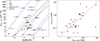 |
Fig. 6. Left: Same as Figure 4, but with tmin, ul measured from structure functions. Right: Comparison between tmin, ul measured in the observed frame from PSDs and structure functions. The red dashed line represents the one-to-one relation. |
5. Discussion
As mentioned in Section 3, we used a single power law, rather than a broken power law, to model the TESS PSDs because the previously measured break frequencies are outside the TESS frequency range or close to the lower limit. To check whether our assumption that the effect of high-frequency breaks on the shortest variability timescale measurements is negligible, we fit the AGN PSDs with the broken power-law model with the high-frequency breaks measured by Yuk & Dai (2025). We found that the shortest variability timescale measurements using single power law and broken power law are consistent.
We measured the shortest AGN optical variability timescale by modelling the TESS PSD as the power law plus a constant noise, where the power law component was detected above the noise and the systematics. Thus, the shortest actual variability timescale might be even shorter under the noise level. For targets with multiple TESS sectors, we used the shortest tmin, ul value in the subsequent analysis, which might be subject to sector-to-sector and pixel-to-pixel instrumental and observational systematics. Future studies with much larger AGN samples might be able to potentially address these issues in a better way. However, it is also possible that the true shortest variability timescale of the sample is greater than our measured values and our measurements are affected by PSD bleeding. Thus, we examined the simulated light curves with an underlying PSD of cutoff power law, where the power is zero (or no variability) past the cutoff frequency, where the cutoff frequency is lower than our detected νmax. This simulates the scenario where no variability is present below the set timescale. Using the method of Timmer & Koenig (1995), we simulated light curves with the following PSD,
 (7)
(7)
where P is the power, α is the power law index, and νc is the cutoff frequency. We simulated the continuous light curves, applied observations windows of TESS, and added measurement noises based on typical errorbar sizes of TESS light curves. Figure 7 shows an example of PSDs of an actual TESS light curve and a simulated light curve. For the simulated PSD, a discontinuity at the cutoff frequency is clearly visible, but this is not seen in the observed PSD measurements.
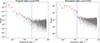 |
Fig. 7. Left: PSD of an actual TESS light curve (NGC 3783 sector 36). The blue dashed line indicates the shortest detected variability timescale. Right: PSD of a simulated light curve with α = 1.8 and νc = 1.5 day−1. The blue dashed line indicates νc. |
To quantify the difference between the two PSD shapes, we simulated 100 light curves with νc = 1.5 day−1 and α = 1.8. We fit two models to real and simulated PSDs and computed the difference in χ2. The first model is a simple power law plus white noise model (Equation (1)), and the second model is a discontinuous power law,
 (8)
(8)
where A1 and A2 are the amplitudes at νc, with A1 ≥ A2, while α1 and α2 are power law indices, νc is the cutoff frequency, and C is the white noise term. This model is designed to detect a discontinuity in the PSD. If the PSD is continuous, A1 should approach A2 and α1 should approach α2, so the fitting results and χ2 should be similar to fitting to Equation (1). The distributions of Δχ2/χ2 is shown on Figure 8. For PSDs retrieved from the actual data, the difference peaks at zero, suggesting that those PSDs are continuous. However, for PSDs from simulated light curves, Δχ2/χ2 peaks at about −0.4, meaning χ2 improves by about 40% by using the discontinuous power law, suggesting that there exist a significant discontinuity in simulated PSDs. With such clear differences between the two distributions, we can confirm that the shortest variability timescale we measured is real.
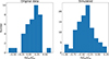 |
Fig. 8. Distributions of Δχ2/χ2 between simple power law model and the discontinuous power law model fits for original data (left) and the simulated data (right). |
There is a number of timescales associated with the optical variability. We computed the various timescales, taking the radial distance from the SMBH, expressed as R, as the theoretical thin disc model accretion disc size (Table 1). We found that the light-crossing timescale of the accretion disc from quasar microlensing measurement or thin disc prediction is the closest to the shortest variability timescale we measure from TESS light curves, of the order of a sub-day. The reverberation mapping disc sizes are largely consistent with quasar microlensing sizes (e.g. Edelson et al. 2015; Jha et al. 2022). The free-fall timescale, which may represent the advection-dominated accretion flows (ADAF) timescale, is roughly of the same order of magnitude as the longest variability timescales measured in the present study. Other timescales, such as the orbital and thermal timescales, are multiple orders of magnitude longer than our measurements.
List of various timescales associated with AGN variability.
Since the light-crossing scale measures a coherently varying emission regions, we find that a significant fraction of AGNs have a coherently varying region that is smaller than the accretion disc size from the thin-disc model prediction or microlensing measurements. This suggests that the short-timescale AGN variability could originate from regions smaller than the accretion disc. We introduce two potential explanations for this observation. Previous studies suggest that the sizes of X-ray and optical emitting regions in AGNs are of the order of 10rg and 100rg, respectively (e.g. Morgan et al. 2008; Dai et al. 2010). For AGNs with the most massive black holes, the optical variability timescale corresponds to less than 10rg. From this, we can hypothesise that the short-timescale optical variability is driven by the inner X-ray emitting region near the accretion disc via reprocessing. The model of X-ray coronal emission being reflected from and reprocessed by the accretion disc has been explored in a number of previous studies (e.g. Pounds et al. 1990; George & Fabian 1991; Shappee et al. 2014b; Papoutsis et al. 2024). For AGNs with less massive black holes, it is possible that the variability timescale measurements are limited by the instrument’s sensitivity more severely than more massive black holes. However, AGNs with such small timescale lengths are limited to a small fraction of our sample. Most of our sample display a variability timescale length that is greater than the measured X-ray emitting region size. Thus, an alternative interpretation is that the optical variability originates from the inhomogeneities in the accretion disc. Some studies theorise that local inhomogeneities cause accretion disc instabilities that lead to AGN variability (e.g. Kawaguchi et al. 1998; Trèvese & Vagnetti 2002; Dexter & Quataert 2012). The physical origin can be turbulence induced by magnetorotational instability (e.g. Balbus & Hawley 1991; Beckwith et al. 2011) or magnetic reconnection due to various physics (e.g. Ball et al. 2018; Ripperda et al. 2020).
Although we did not find a statistically significant correlation between the power-law index and the luminosity, the visual inspection and the correlation coefficient hint at a potentially weak anti-correlation. Previous Kepler PSD studies have indicated such an anti-correlation (Smith et al. 2018). Other studies have reported that the AGN variability amplitude is anti-correlated with black hole mass (e.g. Lu & Yu 2001; Papadakis 2004; MacLeod et al. 2010) and luminosity (e.g. Wang et al. 2022; Kovacevic et al. 2025), which could explain the anti-correlation we observed with the power-law index, assuming similar variability amplitudes.
We also note that a few narrow line Seyfert 1 galaxies were included in our sample; however, we did not find a significant distinction from other Seyfert 1 galaxies. We excluded the jet contribution mostly through the radio loudness parameter. However, there can be jetted AGN with a radio loudness parameter that is below the threshold. We identified a few of them and we note that their short variability can be assumed from the jet. Finally, most of the targets in our sample are truly non-jetted.
6. Conclusion
We examined TESS light curves of 47 type 1 radio-quiet Seyfert galaxies to examine their short-timescale variability. We computed the PSDs of the sample and by comparing to the white noise and systematic variability measured by the upper limits of quiescent galaxies’ PSDs, we measured the shortest detected variability timescale to be log(tmin, ul/h) = 0.85 ± 0.55, or, in units of rg, log(ctmin, ul/rg) = 2.31 ± 0.88. We scaled our variability timescales by the speed of light and compared them to the theoretical and measured accretion disc sizes. As a result, we found that our light-crossing scales are typically smaller.
AGNs exhibiting optical variability in such short timescales can be interpreted in two primary ways. As such short timescales are correlated small lengths (i.e. comparable or smaller than the theoretical and observed accretion disc size), the optical variability may be driven by small-scale sources. One possibility is that the X-ray corona drives the optical variability by reprocessing. Alternatively, inhomogeneities in the accretion disc due to magnetic turbulence or reconnection could cause the detected short-timescale optical variability. This study demonstrates that short-term variability analysis of AGNs can provide a unique way to study the spatial properties of AGNs and the origin of the variability.
We measured the power-law indices as α = 2.0 ± 0.2 and detected weak anti-correlations with the black hole mass and luminosity, consistently with previous studies.
Acknowledgments
We thank the anonymous referee for helpful feedback throughout the review process. We would like to acknowledge NASA funds 80NSSC22K0488, 80NSSC23K0379 and NSF fund AAG2307802.
References
- Aranzana, E., Körding, E., Uttley, P., Scaringi, S., & Bloemen, S. 2018, MNRAS, 476, 2501 [Google Scholar]
- Balbus, S. A., & Hawley, J. F. 1991, ApJ, 376, 214 [Google Scholar]
- Ball, D., Özel, F., Psaltis, D., Chan, C.-K., & Sironi, L. 2018, ApJ, 853, 184 [NASA ADS] [CrossRef] [Google Scholar]
- Bauer, A., Baltay, C., Coppi, P., et al. 2009, ApJ, 696, 1241 [NASA ADS] [CrossRef] [Google Scholar]
- Beckwith, K., Armitage, P. J., & Simon, J. B. 2011, MNRAS, 416, 361 [NASA ADS] [Google Scholar]
- Bennert, V. N., Treu, T., Ding, X., et al. 2021, ApJ, 921, 36 [NASA ADS] [CrossRef] [Google Scholar]
- Bentz, M. C., & Katz, S. 2015, PASP, 127, 67 [Google Scholar]
- Bentz, M. C., Walsh, J. L., Barth, A. J., et al. 2009, ApJ, 705, 199 [NASA ADS] [CrossRef] [Google Scholar]
- Burke, C. J., Shen, Y., Chen, Y.-C., et al. 2020, ApJ, 899, 136 [Google Scholar]
- Burke, C. J., Shen, Y., Blaes, O., et al. 2021, Science, 373, 789 [NASA ADS] [CrossRef] [Google Scholar]
- Chiaberge, M., & Marconi, A. 2011, MNRAS, 416, 917 [Google Scholar]
- Czerny, B. 2006, ASP Conf. Ser., 360, 265 [NASA ADS] [Google Scholar]
- Dai, X., Kochanek, C. S., Chartas, G., et al. 2010, ApJ, 709, 278 [Google Scholar]
- Dexter, J., & Quataert, E. 2012, MNRAS, 426, L71 [CrossRef] [Google Scholar]
- Dingler, R., & Smith, K. L. 2024, ApJ, 973, 10 [Google Scholar]
- Dogruel, M. B., Dai, X., Guerras, E., Cornachione, M., & Morgan, C. W. 2020, ApJ, 894, 153 [Google Scholar]
- Edelson, R., & Nandra, K. 1999, ApJ, 514, 682 [NASA ADS] [CrossRef] [Google Scholar]
- Edelson, R., Gelbord, J. M., Horne, K., et al. 2015, ApJ, 806, 129 [NASA ADS] [CrossRef] [Google Scholar]
- Fabian, A. C., Lohfink, A., Kara, E., et al. 2015, MNRAS, 451, 4375 [Google Scholar]
- Fausnaugh, M. M., Vallely, P. J., Kochanek, C. S., et al. 2021, ApJ, 908, 51 [NASA ADS] [CrossRef] [Google Scholar]
- George, I. M., & Fabian, A. C. 1991, MNRAS, 249, 352 [Google Scholar]
- González-Martín, O. 2018, ApJ, 858, 2 [Google Scholar]
- González-Martín, O., & Vaughan, S. 2012, A&A, 544, A80 [NASA ADS] [CrossRef] [EDP Sciences] [Google Scholar]
- Goyal, A., Gopal-Krishna, Wiita, P. J., et al. 2012, A&A, 544, A37 [NASA ADS] [CrossRef] [EDP Sciences] [Google Scholar]
- Goyal, A., Gopal-Krishna, Paul J., W., Stalin, C. S., & Sagar, R. 2013, MNRAS, 435, 1300 [CrossRef] [Google Scholar]
- Jarrett, T. H., Chester, T., Cutri, R., et al. 2000, AJ, 119, 2498 [Google Scholar]
- Jha, V. K., Joshi, R., Chand, H., et al. 2022, MNRAS, 511, 3005 [NASA ADS] [CrossRef] [Google Scholar]
- Kawaguchi, T., Mineshige, S., Umemura, M., & Turner, E. L. 1998, ApJ, 504, 671 [NASA ADS] [CrossRef] [Google Scholar]
- Kelly, B. C., Bechtold, J., & Siemiginowska, A. 2009, ApJ, 698, 895 [Google Scholar]
- Kochanek, C. S., Shappee, B. J., Stanek, K. Z., et al. 2017, PASP, 129, 104502 [Google Scholar]
- Koss, M., Trakhtenbrot, B., Ricci, C., et al. 2017, ApJ, 850, 74 [Google Scholar]
- Kovacevic, N., Dai, X., Yuk, H., et al. 2025, ApJ, 985, 177 [Google Scholar]
- Kozłowski, S. 2016, ApJ, 826, 118 [CrossRef] [Google Scholar]
- Kumar, P., Gopal-Krishna, & Hum, C. 2015, MNRAS, 448, 1463 [Google Scholar]
- Lomb, N. R. 1976, Ap&SS, 39, 447 [Google Scholar]
- Lu, Y., & Yu, Q. 2001, MNRAS, 324, 653 [NASA ADS] [CrossRef] [Google Scholar]
- Lynden-Bell, D. 1969, Nature, 223, 690 [NASA ADS] [CrossRef] [Google Scholar]
- MacLeod, C. L., Ivezić, Ž., Kochanek, C. S., et al. 2010, ApJ, 721, 1014 [Google Scholar]
- Markowitz, A., Edelson, R., Vaughan, S., et al. 2003, ApJ, 593, 96 [NASA ADS] [CrossRef] [Google Scholar]
- McHardy, I. M., Papadakis, I. E., Uttley, P., Page, M. J., & Mason, K. O. 2004, MNRAS, 348, 783 [NASA ADS] [CrossRef] [Google Scholar]
- Middei, R., Vagnetti, F., Bianchi, S., et al. 2017, A&A, 599, A82 [NASA ADS] [CrossRef] [EDP Sciences] [Google Scholar]
- Morgan, C. W., Kochanek, C. S., Dai, X., Morgan, N. D., & Falco, E. E. 2008, ApJ, 689, 755 [Google Scholar]
- Morgan, C. W., Kochanek, C. S., Morgan, N. D., & Falco, E. E. 2010, ApJ, 712, 1129 [Google Scholar]
- Mushotzky, R. F., Edelson, R., Baumgartner, W., & Gandhi, P. 2011, ApJ, 743, L12 [NASA ADS] [CrossRef] [Google Scholar]
- Ojha, V., Krishna, G., & Chand, H. 2019, MNRAS, 483, 3036 [NASA ADS] [CrossRef] [Google Scholar]
- Paolillo, M., & Papadakis, I. 2025, arXiv e-prints [arXiv:2506.23899] [Google Scholar]
- Papadakis, I. E. 2004, MNRAS, 348, 207 [NASA ADS] [CrossRef] [Google Scholar]
- Papoutsis, M., Papadakis, I. E., Panagiotou, C., Dovčiak, M., & Kammoun, E. 2024, A&A, 691, A60 [NASA ADS] [CrossRef] [EDP Sciences] [Google Scholar]
- Peng, Z., Gu, Q., Melnick, J., & Zhao, Y. 2006, A&A, 453, 863 [NASA ADS] [CrossRef] [EDP Sciences] [Google Scholar]
- Peterson, B. M. 1993, PASP, 105, 247 [NASA ADS] [CrossRef] [Google Scholar]
- Peterson, B. M., Bentz, M. C., Desroches, L.-B., et al. 2005, ApJ, 632, 799 [NASA ADS] [CrossRef] [Google Scholar]
- Pounds, K. A., Nandra, K., Stewart, G. C., George, I. M., & Fabian, A. C. 1990, Nature, 344, 132 [NASA ADS] [CrossRef] [Google Scholar]
- Pozo Nuñez, F., Ramolla, M., Westhues, C., et al. 2015, A&A, 576, A73 [NASA ADS] [CrossRef] [EDP Sciences] [Google Scholar]
- Rani, B., Kim, J., Papadakis, I., et al. 2025, ApJ, 981, L18 [Google Scholar]
- Ricker, G. R., Winn, J. N., Vanderspek, R., et al. 2015, JATIS, 1, 014003 [Google Scholar]
- Ripperda, B., Bacchini, F., & Philippov, A. A. 2020, ApJ, 900, 100 [NASA ADS] [CrossRef] [Google Scholar]
- Romero, G. E., Cellone, S. A., & Combi, J. A. 1999, A&AS, 135, 477 [NASA ADS] [CrossRef] [EDP Sciences] [Google Scholar]
- Scargle, J. D. 1982, ApJ, 263, 835 [Google Scholar]
- Shakura, N. I., & Sunyaev, R. A. 1973, A&A, 24, 337 [NASA ADS] [Google Scholar]
- Shappee, B., Prieto, J., Stanek, K. Z., et al. 2014a, AAS Meet. Abstr., 223, 236.03 [Google Scholar]
- Shappee, B. J., Prieto, J. L., Grupe, D., et al. 2014b, ApJ, 788, 48 [Google Scholar]
- Skrutskie, M. F., Cutri, R. M., Stiening, R., et al. 2006, AJ, 131, 1163 [NASA ADS] [CrossRef] [Google Scholar]
- Smith, K. L., Mushotzky, R. F., Boyd, P. T., et al. 2018, ApJ, 857, 141 [NASA ADS] [CrossRef] [Google Scholar]
- Tarrant, A., Hinkle, J., Shappee, B., et al. 2025, arXiv e-prints [arXiv:2501.12444] [Google Scholar]
- Timmer, J., & Koenig, M. 1995, A&A, 300, 707 [NASA ADS] [Google Scholar]
- Trèvese, D., & Vagnetti, F. 2002, ApJ, 564, 624 [Google Scholar]
- Tueller, J., Mushotzky, R. F., Barthelmy, S., et al. 2008, ApJ, 681, 113 [NASA ADS] [CrossRef] [Google Scholar]
- Uttley, P., McHardy, I. M., & Papadakis, I. E. 2002, MNRAS, 332, 231 [Google Scholar]
- Vallely, P. J., Kochanek, C. S., Stanek, K. Z., Fausnaugh, M., & Shappee, B. J. 2021, MNRAS, 500, 5639 [Google Scholar]
- Wang, J.-M., & Zhang, E.-P. 2007, ApJ, 660, 1072 [NASA ADS] [CrossRef] [Google Scholar]
- Wang, H.-T., Su, Y.-P., Ge, X., Chen, Y.-Y., & Yu, X.-L. 2022, Res. Astron. Astrophys., 22, 015014 [Google Scholar]
- Yang, Y., Ma, B., & Chen, C. 2024, Universe, 10, 434 [Google Scholar]
- Yuk, H., & Dai, X. 2025, A&A, 698, A105 [NASA ADS] [CrossRef] [EDP Sciences] [Google Scholar]
- Yuk, H., Dai, X., Jayasinghe, T., et al. 2022, ApJ, 930, 110 [NASA ADS] [CrossRef] [Google Scholar]
- Zhou, X.-L., Zhang, S.-N., Wang, D.-X., & Zhu, L. 2010, ApJ, 710, 16 [NASA ADS] [CrossRef] [Google Scholar]
- Zu, Y., Kochanek, C. S., & Peterson, B. M. 2011, ApJ, 735, 80 [NASA ADS] [CrossRef] [Google Scholar]
Appendix A: Properties of the sample
Here, we present the properties of the sample of 47 Seyfert 1 galaxies used in this study, including redshift, V-band luminosity, black hole mass, and TESS sectors used for the light curve analysis (Table A.1).
Summary of the radio-quiet Seyfert 1 galaxy sample
All Tables
All Figures
|
Fig. 1. Left: Systematics of TESS survey and light curve extraction technique indicated by the PSDs of non-variable galaxy light curves, where the y-axis is the scaled power relative to the constant white noise. Each gray line indicates the power law plus white noise fit for an individual galaxy’s light curve, the black line represents the mean galaxy PSD, and the red and yellow shaded areas represent the one-sigma and three-sigma limits, respectively. Right: Comparison between Seyfert 1 AGN, ESO 362-G018, Sector 5 PSD (which has the measured tmin, ul value equal to the median of the AGN sample), and the upper limits of galaxies as a representative to illustrate the measurement of the shortest detected variability timescale. The text next to the PSD lists the parameters for the best fit. The PSDs in both panels are normalised by their respective noise levels. |
| In the text | |
|
Fig. 2. Left: Distribution of quiescent galaxies’ structure functions, normalised by the noise level, similar to Figure 1 left. Right: Comparison of structure functions of galaxies and NGC 931 sector 18 to demonstrate the smallest variability timescale measurement. |
| In the text | |
|
Fig. 3. Left: Distribution of the shortest detected TESS variability timescales of the sample. Right: Histogram showing the distribution of ctmin, ul in terms of rg. |
| In the text | |
|
Fig. 4. Distribution of the shortest detected TESS variability timescales of the sample, plotted against the black hole mass. The blue dashed lines indicate the different values of gravitational radii for the given black hole mass, and the green and red solid lines indicate the theoretical and measured accretion disc and corona sizes from literature (Shakura & Sunyaev 1973; Morgan et al. 2010; Dogruel et al. 2020). |
| In the text | |
|
Fig. 5. Top left: Distribution of the power law indices for the PSD power law fit. Black hole mass (top right), LV/LEdd (bottom left), and V-band luminosity (bottom right) plotted against the power law index. |
| In the text | |
|
Fig. 6. Left: Same as Figure 4, but with tmin, ul measured from structure functions. Right: Comparison between tmin, ul measured in the observed frame from PSDs and structure functions. The red dashed line represents the one-to-one relation. |
| In the text | |
|
Fig. 7. Left: PSD of an actual TESS light curve (NGC 3783 sector 36). The blue dashed line indicates the shortest detected variability timescale. Right: PSD of a simulated light curve with α = 1.8 and νc = 1.5 day−1. The blue dashed line indicates νc. |
| In the text | |
|
Fig. 8. Distributions of Δχ2/χ2 between simple power law model and the discontinuous power law model fits for original data (left) and the simulated data (right). |
| In the text | |
Current usage metrics show cumulative count of Article Views (full-text article views including HTML views, PDF and ePub downloads, according to the available data) and Abstracts Views on Vision4Press platform.
Data correspond to usage on the plateform after 2015. The current usage metrics is available 48-96 hours after online publication and is updated daily on week days.
Initial download of the metrics may take a while.