| Issue |
A&A
Volume 709, May 2026
|
|
|---|---|---|
| Article Number | A41 | |
| Number of page(s) | 15 | |
| Section | Stellar structure and evolution | |
| DOI | https://doi.org/10.1051/0004-6361/202558097 | |
| Published online | 01 May 2026 | |
Impact of stellar rotation on type II supernova progenitor masses determined from pre-explosion imaging
1
Instituto de Astrofísica de La Plata (IALP), CCT-CONICET-UNLP, Paseo del Bosque S/N, B1900FWA, La Plata, Argentina
2
Facultad de Ciencias Astronómicas y Geofísicas – UNLP, Paseo del Bosque S/N, B1900FWA, La Plata, Argentina
★ Corresponding author: This email address is being protected from spambots. You need JavaScript enabled to view it.
Received:
13
November
2025
Accepted:
18
March
2026
Abstract
The initial masses of red supergiant type II supernova (SN II) progenitors are commonly inferred from pre-explosion imaging by converting the progenitor luminosity into an initial mass estimate using non-rotating stellar evolution models. However, stellar rotation affects the evolution and may influence these estimates. We investigated how the observed distribution of rotational velocities in massive stars influences the progenitor initial masses of SNe II inferred from pre-SN imaging. We compared initial mass estimates obtained from non-rotating models with those derived from rotating models, in which the initial rotational velocities of the stellar models are sampled from the observed distribution. We analysed the inferred progenitor initial masses by (i) comparing the results for each SN individually, (ii) examining the overall probability density function, (iii) constructing the cumulative distribution function, and (iv) determining the upper initial-mass boundary. In all cases, the distributions obtained from rotating models are slightly shifted towards lower masses, although the differences remain smaller than the typical uncertainties. When using the observed distribution of initial rotational velocities for massive stars, we infer an upper initial-mass limit for SN II progenitors of 20.4+2.3−1.9 M⊙. Taken together, these analyses demonstrate that stellar rotation has only a modest impact on progenitor mass estimates from pre-SN imaging within the current observational and model uncertainties when the observed distribution of initial rotational velocities is taken into account. Therefore, adopting this distribution leads to small differences compared to non-rotating models.
Key words: stars: evolution / stars: massive / stars: rotation / supernovae: general
Member of the Carrera del Investigador Científico, Comisión de Investigaciones Científicas de la Provincia de Buenos Aires (CIC-PBA), Argentina.
© The Authors 2026
 Open Access article, published by EDP Sciences, under the terms of the Creative Commons Attribution License (https://creativecommons.org/licenses/by/4.0), which permits unrestricted use, distribution, and reproduction in any medium, provided the original work is properly cited.
This article is published in open access under the Subscribe to Open model. This email address is being protected from spambots. You need JavaScript enabled to view it. to support open access publication.
1. Introduction
Type II supernovae (SNe II1) are the explosive deaths of massive stars (≳9 M⊙) through the core-collapse mechanism and are characterised by spectra with prominent hydrogen features (Minkowski 1941; Filippenko et al. 1993). The presence of such hydrogen features indicates that the progenitor stars retained a substantial fraction of their hydrogen envelopes throughout their evolution up to the core-collapse event. This scenario has been further supported by the identification of red supergiant (RSG) stars in archival pre-explosion images at the locations of SN II events, providing direct evidence that RSGs constitute the progenitors of SNe II (Smartt 2015; Van Dyk 2025).
Type II SNe are the most common type of core-collapse SN (CCSN) in nature (Shivvers et al. 2017; Pessi et al. 2025). However, the exact ranges of the physical properties of their progenitors remain uncertain, particularly their initial masses. Several methods have been used to estimate progenitor initial masses, including nebular spectral modelling (e.g. Jerkstrand et al. 2015; Fang et al. 2025) and light-curve modelling (e.g. Morozova et al. 2018; Martinez et al. 2020), both of which link post-explosion observables to progenitor mass through inference methods that rely on stellar evolution models. The study of stellar populations at SN explosion sites (Maund 2017; Williams et al. 2018) also provides constraints on progenitor masses.
While previous approaches relied on post-explosion observables or stellar population studies, a more direct method for estimating progenitor properties is to detect individual progenitors in pre-explosion images. This allows the measurement of their luminosity and effective temperature prior to the SN event. The progenitor luminosity is obtained from fits to the spectral energy distribution or using bolometric corrections (e.g. Davies & Beasor 2018; Van Dyk et al. 2019). The next step is to convert the pre-explosion progenitor luminosity into an initial mass estimate using stellar evolution models.
The estimation of the initial masses of observed SN II progenitors is generally consistent with estimates obtained from post-explosion techniques, such as light-curve modelling and the analysis of nebular spectra (e.g. Jerkstrand et al. 2015; Eldridge et al. 2019). In particular, Eldridge et al. (2019) produced SN light-curve models using progenitors computed with the STARS stellar evolution code (Eldridge & Tout 2004), the same code that has been used to link observed progenitor luminosities to initial masses (Smartt 2015), finding consistent initial-mass estimates from the two approaches.
Estimations of the initial mass from the pre-explosion progenitor luminosity have typically required publicly available grids of stellar evolution models. These are typically computed either without rotation or assuming a fixed fraction of the critical velocity at the zero-age main sequence (ZAMS), most commonly Ωini/Ωcrit = 0.4 (where Ωini and Ωcrit are the initial and critical surface angular velocities, respectively), using codes such as KEPLER (Woosley & Heger 2007), STARS (Eldridge et al. 2008), GENEVA (Ekström et al. 2012), and MESA (Paxton et al. 2011) through the MIST project (Choi et al. 2016). Hence, the available rotating grids usually represent only a single fixed value rather than a range of initial rotational velocities. However, stellar rotational velocities at the ZAMS span a wide range (Huang et al. 2010; Holgado et al. 2022).
Rotation has a major impact on the evolution of massive stars. While rotation increases wind mass-loss rates through centrifugal effects (Maeder & Meynet 2000; Langer 2012), its primary effect is the enhancement of internal chemical mixing. Rotational instabilities transport fresh fuel into the core, thereby extending the duration of the nuclear burning phases and increasing core masses, while also affecting surface abundances and nucleosynthetic yields, among other effects (Maeder & Meynet 2000). Variations in the rotation rate alter the amount of internal mixing and therefore the mass of the helium core. Because the helium core mass sets the final stellar luminosity, rotation – via enhanced mixing – changes the initial-mass–to–final-luminosity relation.
In this work we estimated the initial masses of SN II progenitors from their pre-explosion luminosities by explicitly incorporating the observed distribution of stellar rotational velocities at the ZAMS. Our main goal was to quantify the differences between this approach and the traditional method based on non-rotating models, in order to assess the impact of the observed initial velocity distribution on the inferred population of SN II progenitors.
In Sect. 2 we provide a brief description of the SN II sample. Section 3 presents the grids of stellar evolution models and the methodology used to estimate the progenitor initial-mass distributions. The results obtained with non-rotating models and with rotating models based on the observed initial rotational velocities of massive stars are presented in Sect. 4. In Sect. 5 we perform statistical comparisons between the initial-mass distributions obtained from results using rotating and non-rotating models. In Sect. 6 we discuss the key implications of our analysis, such as the nature of low-luminosity progenitors, the current statistical significance of the RSG problem, and the potential role of binary interaction channels. Finally, Sect. 7 summarises our main conclusions. Additional figures not included in the main body of the manuscript are provided in the appendix.
2. Sample of SN II progenitors
In this work we aim to determine the differences in SN II progenitor initial masses inferred from pre-SN imaging when constraining with rotating and non-rotating models. In this context, the key observable is the pre-SN luminosity, which is converted into an initial mass through stellar evolution models.
We therefore collected a sample of SN II progenitors detected in pre-SN images with direct luminosity estimates, excluding those with only upper limits. Based on this criterion, we initially gathered 24 SNe II from the literature, of which some were discarded. Two of the progenitors we excluded are those of SN 2003gd and SN 2005cs. The luminosities of these stars have been estimated based only on data from the Hubble Space Telescope F814W band and, thus, may be significantly underestimated (Beasor et al. 2025). In addition, the progenitor of SN 2020jfo remains uncertain (Van Dyk 2025), as the fit to its observed spectral energy distribution is consistent with a star below the mass range expected to explode as either a CCSN or an electron-capture SN (ECSN), even when assuming a dust-obscured RSG model (Kilpatrick et al. 2023). Therefore, our final sample consists of 21 SN II progenitors, which are listed in Table 1 together with their pre-SN luminosities.
Pre-SN luminosities of SN II progenitors in the sample analysed in this work.
3. Methods
In this section we describe the methods used to estimate the initial masses of SN II progenitors. Section 3.1 presents the computation of stellar evolution models for rotating massive stars and the impact of rotation on their pre-SN luminosities. Section 3.2 details the observationally derived distribution of initial rotational velocities for massive stars. Finally, Sect. 3.3 describes the Monte Carlo (MC) approach used to combine the observed progenitor luminosities and rotational velocities with the model grids to infer the progenitor initial-mass distributions.
3.1. Modelling rotating massive stars
To estimate progenitor initial masses, it is necessary to compare the observed pre-SN luminosity with that predicted by stellar evolution models. For this purpose, we computed evolutionary models of single massive stars at solar metallicity (Z⊙ = 0.0154; Asplund et al. 2021) with the public stellar evolution code MESA2, version 24.08.1 (Paxton et al. 2011, 2013, 2015, 2018, 2019; Jermyn et al. 2023). Each stellar model was evolved from the ZAMS until core carbon depletion, which we defined as the stage when central carbon mass fraction drops below 0.01.
Wind mass loss rates for massive stars were computed following the latest prescriptions: Björklund et al. (2023) for hot stars, and Wen et al. (2024) for cool stars. In the transition region, the wind mass loss rate is a combination of the two prescriptions using the same method as in the ‘Dutch’ wind scheme defined in MESA. We adopted the wind prescriptions from Wen et al. (2024), which were derived for RSGs in the Large Magellanic Cloud, even though our stellar models assume solar metallicity. This is justified because previous studies indicate that RSG wind mass-loss rates show little dependence on metallicity, with no strong correlation between the two (Goldman et al. 2017; Antoniadis et al. 2025).
We used the Ledoux criterion to determine the convective regions and set the mixing length parameter to αmlt = 2.0. The semi-convection and thermohaline mixing efficiency parameters were both set to 1.0 (Kippenhahn et al. 1980; Langer et al. 1983). Convective-core overshooting was treated with the step formalism during hydrogen- and helium-core burning, adopting overshooting parameters of αos = 0.15 (Martins & Palacios 2013) and 0.03 (Li et al. 2019) pressure scale heights, respectively. The hydrogen-core overshooting parameter was calibrated by Martins & Palacios (2013) through comparisons with the observed width of the main sequence using rotating stellar models with different overshooting prescriptions. While this calibration partially accounts for the additional mixing induced by rotation, it is based on models computed with a single initial rotational velocity (or a fixed fraction of the critical velocity), rather than a distribution of rotation rates. During carbon burning, we adopted the exponential approach implemented in MESA to account for convective overshooting, with a parameter f = 0.004 (Farmer et al. 2016).
There are currently two approaches to treating chemical mixing and angular momentum transport caused by rotationally induced instabilities in one-dimensional stellar evolution models: the diffusion approximation (Endal & Sofia 1978; Heger et al. 2000) and the diffusion–advection approach (Zahn 1992). MESA adopts the former (Paxton et al. 2013). The rotationally induced instabilities included in our models are: dynamical shear instability, Solberg–Høiland instability, secular shear instability, Eddington−Sweet circulation, and Goldreich–Schubert–Fricke instability (see Heger et al. 2000 for details). Additionally, we included the effects of internal magnetic fields following the Spruit–Tayler dynamo approach (Spruit 2002; Heger et al. 2005; Paxton et al. 2013). In the diffusion approximation, two free parameters require calibration: fc, the ratio of the turbulent viscosity to the diffusion coefficient, and fμ, which describes the sensitivity of rotationally induced mixing to μ-gradients. We adopted fc = 1/30 and fμ = 0.05, following Heger et al. (2000).
Using the stellar evolution parameters described above, we computed models varying the initial mass and the initial rotational surface velocity. The initial surface velocities were chosen in the range 0–600 km s−1, with steps of 50 km s−1. The upper limit is motivated by the observed velocity distribution of massive stars (see Sect. 3.2). The models were assumed to rotate uniformly on the ZAMS.
The minimum initial mass in our grids was set by the lowest-mass star capable of producing a CCSN at the end of its evolution. We adopted neon ignition – either central or off-centre – as the criterion defining this limit, since stars that ignite neon are generally expected to undergo core collapse rather than end as oxygen–neon (ONe) white dwarfs or ECSNe (Nomoto et al. 1984; Kippenhahn et al. 2013; Limongi et al. 2024). We note that ECSNe are expected to arise from slightly lower initial masses and would observationally appear as SNe II, which are the events considered in this work. However, ECSNe are predicted to occur over a relatively narrow initial-mass range, of about 0.5 M⊙ (Poelarends et al. 2008; Limongi et al. 2024). Including this channel could slightly shift the inferred initial-mass distribution towards lower masses, but it is not expected to significantly affect our results. Our models place the minimum initial mass for producing a SN II explosion at 9 M⊙3. Therefore, we set the minimum initial mass to 9 M⊙, independent of the initial surface rotational velocity.
The maximum initial mass depends on the initial surface velocity. For grids with velocities between 0 and 300 km s−1, it was 30 M⊙. Within this velocity range, initially more massive stars still retain a significant hydrogen-rich envelope at the end of evolution and are therefore expected to explode as SNe II. However, their final luminosities exceed those inferred for observed SN II progenitors, and we did not consider them further. For higher initial surface velocities, the maximum initial mass was set by the condition that the star retains a significant hydrogen-rich envelope at the end of its evolution, while more massive stars lose almost their entire envelope and would not end their lives as SNe II. This dependence arises because rotation affects stellar evolution through enhanced mass loss and chemical mixing (Maeder 2009). Increased mixing supplies more hydrogen to the core, producing more massive helium cores. Consequently, these stars are more luminous and develop stronger winds, which act together to the intrinsic increased mass loss to reduce the hydrogen-rich envelope mass. As a result, the maximum initial mass decreases with increasing initial surface velocity. The maximum initial-mass values for each initial velocity are listed in Table 2.
Maximum initial mass across the computed grids for different initial surface velocities.
Figure 1 shows Hertzsprung–Russell (HR) diagrams for a subsample of our models. The left panel presents evolutionary tracks for non-rotating models, while the right panel shows tracks for rotating 10, 15, 20, and 25 M⊙ models at different initial rotational velocities, illustrating the effects of stellar rotation. Additionally, Fig. A.1 shows HR diagrams of models spanning the entire range of initial masses and a selected set of initial rotational velocities.
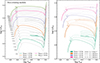 |
Fig. 1. HR diagrams for a subsample of stellar models. Left panel: Non-rotating models. Coloured lines correspond to models with initial masses of 10, 15, 20, and 25 M⊙, and the remaining models are shown as faint grey lines. Right panel: Evolutionary tracks for stars with initial masses of 10, 15, 20, and 25 M⊙ and different initial rotational velocities, as indicated in the panel label. We note that the model with an initial mass of 25 M⊙ and an initial rotational velocity of 400 km s−1 lies outside the parameter space of the current study (see Table 2). |
The evolution of rotating models follows the expected behaviour relative to non-rotating models. On the ZAMS and during the early stages of the main-sequence evolution, rotation induces a shift of the tracks towards lower luminosities and effective temperatures, primarily due to the reduction of the effective gravity. As evolution proceeds, the evolutionary tracks of rotating models become more luminous than those of non-rotating models. This results from rotational mixing during the main-sequence evolution. On the one hand, enhanced mixing supplies fresh hydrogen to the hydrogen-burning convective core, thereby producing more massive helium cores and more luminous stars. On the other hand, rotational mixing transports helium and other hydrogen-burning products to the surface, reducing the opacity and contributing to an increase in stellar luminosity. Owing to the more massive helium core, the post-main sequence evolution resembles that of an initially more massive star, resulting in higher luminosities compared to non-rotating models. For further details on the evolution of rotating stars the reader is referred to, for example Meynet & Maeder (2000) and Chieffi & Limongi (2013).
In the current work we focused primarily on the final luminosity of each model, as it will be compared with the observed progenitor luminosity to estimate the initial mass. Figure 2 shows the final luminosity for a subset of the models. As expected, more massive stars reach higher luminosities at the end of their evolution. Additionally, due to the rotational effects described above, more rapidly rotating stars attain higher final luminosities at a given initial mass. We note that, at a fixed final luminosity, the range of initial masses increases towards higher luminosities. For instance, at log L = 4.8, the inferred initial mass spans approximately 2 M⊙, across the considered rotation rates. This spread increases to about 3 M⊙ at log L = 5.0, and to roughly 8 M⊙ at log L = 5.5, implying larger uncertainties at higher luminosities. At low and intermediate luminosities, the range of inferred initial masses is comparable to that found by Eldridge & Tout (2004), who showed that similar mass spreads arise when considering models with and without convective core overshooting. This highlights that uncertainties in stellar evolution modelling, such as chemical mixing processes, play an important role in setting the spread of inferred progenitor initial masses. Additionally, Eldridge & Tout (2004) found comparable mass spreads resulting from variations in the initial metallicity. We note that our analysis is restricted to solar-metallicity models. Some stellar properties at core carbon depletion for the non-rotating models are presented in Table 3.
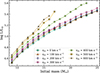 |
Fig. 2. Stellar luminosities at core carbon depletion for a range of initial masses and surface velocities. Only a subset of the models is shown, for visualisation purposes. |
Properties of non-rotating stellar models at the end of core carbon burning.
3.2. Initial rotational velocity distribution of massive stars
When using the initial-mass–to–final-luminosity relation to infer the mass of a SN progenitor, previous studies typically rely on either non-rotating models or rotating models computed with an initial surface velocity set to a fixed fraction of the critical value (e.g. Davies & Beasor 2018, 2020). In the latter case, a value of Ωini/Ωcrit = 0.4 is commonly adopted, motivated by the peak in the observed rotational velocity distribution of young B-type stars (Huang et al. 2010). In this work, rather than assuming that all stars initially rotate at a fixed fraction of the critical velocity, we accounted for the full observed distribution of initial rotational velocities for massive stars at the ZAMS.
For this purpose, we used the projected rotational velocities (v sin i) of single Galactic O-type stars presented by Holgado et al. (2022). In particular, we adopted the subsample defined in their study corresponding to stars with initial masses below 32 M⊙, which is consistent with the mass range of our model grid. In addition, we restricted the sample to stars with surface gravities log g > 3.7 dex in order to focus on young stars (see Fig. 8c of Holgado et al. 2022), thereby approximating a rotational velocity distribution at the ZAMS. Given that Holgado et al. (2022) reported projected rotational velocities, we applied the deconvolution algorithm of Lucy (1974) to recover the intrinsic rotational velocity distribution. Figure 3 compares the observed projected distribution with the deconvolved distribution. The latter extends up to ∼600 km s−1, which justifies the choice of the maximum surface velocity adopted in our model grid (Sect. 3.1).
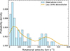 |
Fig. 3. Probability density of rotational velocities. Projected rotational velocities of young Galactic O-type stars from Holgado et al. (2022) with masses below 32 M⊙ are shown as a histogram. The deconvolved distribution, obtained using the method of Lucy (1974), is overplotted as a thick line. |
3.3. Mass distribution inference
In this section we describe the method used to infer the initial-mass distribution of each SN II progenitor in the sample, combining the observed progenitor luminosity with the initial rotational surface velocity. For each SN II progenitor in our sample, we drew a luminosity value from a Gaussian distribution centred on the observed luminosity, with a standard deviation equal to the reported uncertainty (see Table 1). In cases where the luminosity is provided as a range rather than as a value with an associated uncertainty, we adopted the midpoint of the range as the mean of the Gaussian, and set the distance between the midpoint and either boundary of the range equal to three standard deviations. We next sampled a value from the initial rotational velocity distribution described in Sect. 3.2.
In principle, the effective temperatures of observed SN II progenitors could also be compared with those predicted by stellar models. However, we did not include the effective temperature as an additional parameter to infer the progenitor initial mass for the reasons discussed below. On the one hand, the vast majority of our stellar models end their evolution with very similar effective temperatures; therefore, the effective temperature does not provide an additional constraint for the initial-mass estimate. Only a few models deviate significantly from this value, corresponding to stars that evolve bluewards due to their reduced hydrogen envelopes. At the same time, these models exhibit final luminosities that exceed those inferred for observed SN II progenitors, and therefore do not contribute to the inferred initial-mass distribution. On the other hand, the uncertainties in the observed effective temperatures are typically large enough to cover the narrow interval of final effective temperatures predicted by the models. For these reasons, we did not use the effective temperature as an additional constraint in our analysis.
With the sampled progenitor luminosity and initial surface velocity, we used our model grids to infer the corresponding initial mass. We first identified the closest models in the grid to the input values using the cKDTree algorithm from the SciPy Python package, which implements a k-dimensional tree to efficiently organise points in a multi-dimensional parameter space. For the nearest models, we assigned weights based on a Gaussian kernel centred on the target parameters, with the distance in parameter space determining the weight. Finally, the progenitor’s initial mass was obtained by interpolating the models according to these weights. If the input progenitor luminosity is below the minimum in our models, we set the progenitor initial mass to the minimum value in the grid to avoid extrapolating beyond the model range.
In summary, this procedure relates the sampled luminosity and initial surface velocity values to an initial mass estimate through multi-dimensional interpolation of the rotating stellar models. We hereafter refer to this approach as the distribution-based rotating (DBR) models. We repeated this MC procedure 10 000 times for each SN II progenitor, thereby determining the posterior probability distribution of its initial mass.
4. Results
We determined the probability distributions of the initial mass for each SN II progenitor in the sample using the MC method described in Sect. 3.3, combined with the stellar evolutions models presented in Sect. 3.1. For comparison, we also computed results using only non-rotating models4. This allowed us to directly assess the differences with respect to the DBR models, which constitute the main aim of this work.
As an example of our results, Fig. 4 shows the initial-mass distribution of the progenitor of SN 2025pht using the DBR models (i.e. including the initial surface velocity distribution and rotating stellar models). SN 2025pht is the most recent SN II with a detected progenitor in pre-explosion images, and the first to be identified with the James Webb Space Telescope (Kilpatrick et al. 2025). We derived an initial mass of MZAMS = 14.3 ± 1.5 M⊙, consistent with previous estimates (Kilpatrick et al. 2025).
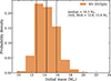 |
Fig. 4. Initial-mass distribution of the progenitor of SN 2025pht using the DBR models. The solid vertical line corresponds to the median of the distribution, and dashed vertical lines are the 16th and 84th percentiles. |
Table 4 lists the 16th, 50th, and 84th percentiles of the posterior distribution of the progenitor initial mass for each SN II in the sample. Results are shown for both the non-rotating and DBR models. Additionally, the initial-mass distributions for the entire SN II sample are shown in Appendix B (Fig. B.1).
Progenitor initial masses from non-rotating and DBR models for each SN II in the sample.
We note that for the progenitor of SN 2022acko the resulting distributions, from both non-rotating and DBR models, are (almost) entirely concentrated at an initial mass value of 9 M⊙. This behaviour arises because the observed progenitor luminosity is significantly lower than the minimum luminosity covered by our models. As described in Sect. 3.3, if during the MC analysis the progenitor luminosity falls below the minimum in the models, we set the progenitor initial mass to the lowest grid value, which is 9 M⊙. For the DBR models, all 10 000 MC trials fall below this luminosity threshold. In the case of non-rotating models, only ∼1% of the trials lie above the minimum model luminosity, resulting in a slightly broader distribution. Although the progenitor luminosity lies below the range covered by our models, it could still be consistent with a CCSN at the lower initial mass limit, or with an ECSN (Van Dyk et al. 2023). We note that post-explosion images, once the SN emission has faded sufficiently, are required to confirm the progenitor through its disappearance.
A similar situation is found for SNe 2008bk, 2009md, 2012A, and 2024afbl, where part of the progenitor luminosity distribution extends below the minimum luminosity of the model grid. This results in the corresponding mass distributions being clustered around the lowest grid value. In Sect. 6.1 we discuss these low-luminosity progenitors in the context of stellar evolution models.
5. Analysis
Having derived individual progenitor masses for each SN II in the sample from non-rotating and DBR models, we next performed a statistical analysis of the complete sample. This analysis included comparisons between the two sets of estimates for each SN, the construction of probability density functions (PDFs) and cumulative distribution functions (CDFs), and the determination of the upper mass boundary.
Figure 5 compares the median values of the initial-mass distributions obtained with non-rotating and DBR models for each SN II progenitor in the sample, with error bars corresponding to the 16th and 84th percentiles. In all cases, the median masses inferred from DBR models are systematically lower than those from non-rotating models. This systematic offset arises from one of the main effects of stellar rotation: enhanced chemical mixing. In rotating models, the increased mixing supplies additional material to the burning core, producing more massive cores. As a result, stars are more luminous throughout their evolution, including the pre-SN stage considered here. This luminosity increase explains the shift towards lower initial masses when adopting DBR models (see also Fig. B.1). Although this trend was expected (e.g. Straniero et al. 2019), in the following we quantify the differences.
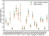 |
Fig. 5. Median of the initial-mass distribution of SN II progenitors in the sample, derived from non-rotating (green dots) and DBR models (orange triangles). Error bars correspond to the 16th and 84th percentiles. |
The smallest differences are found for SNe 2008bk, 2009md, 2012A, and 2024afbl. As discussed in Sect. 4, their inferred progenitor masses are clustered near the lower boundary of the model grid. Excluding these cases, the smallest difference is 0.2 M⊙ for SN 2013ej, while the largest is 1.1 M⊙ for SN 2009hd, with the rest of the sample falling within this range. Thus, the typical range of differences is ∼0.2−1.1 M⊙ (Fig. 5). Moreover, although the distributions obtained with DBR models are shifted towards lower initial masses, the median values always remain within 1σ of those derived from non-rotating models. In general, the shifts in the inferred initial masses are modest, and the distributions largely overlap, indicating that the impact of including rotation is small compared to the typical observational uncertainties.
In the preceding analysis, we compared the initial-mass distributions for each SN II progenitor individually using both procedures. We next examined the PDF of the initial mass by considering all distributions simultaneously. To this end, we estimated the corresponding distribution using a Gaussian kernel density estimator applied to the MC samples described above, implemented with the gaussian_kde function from the SciPy package. Figure 6 shows the resulting PDFs for the non-rotating and DBR models. Although the distribution derived from the DBR models is shifted towards lower initial masses, the differences remain small. To quantify the similarity between the two probability distributions, we computed the Hellinger distance (Hellinger 1909). This metric takes values H between 0 and 1, with H ≈ 0 indicating nearly identical distributions and H ≈ 1 corresponding to very different ones. We obtain H = 0.06, confirming that the two distributions are indeed very similar, consistent with the visual comparison from Fig. 6.
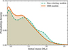 |
Fig. 6. PDFs of the SN II progenitor’s initial mass, derived from non-rotating (dashed green line) and DBR models (solid orange line). |
We next focused on the lower and upper initial-mass boundaries of the distribution (Mlo, Mup). These are key properties commonly derived in SN II progenitor studies, which provide important constraints on the evolutionary pathways of massive stars (e.g. Smartt 2015; Davies & Beasor 2020). To this end, we first constructed the CDF of the progenitor initial masses in our sample, following the approach of Davies & Beasor (2020). For each of the 10 000 MC trials carried out in Sect. 5, we took the initial mass corresponding to each SN II progenitor in the sample and sorted the values in ascending order. This procedure allowed us to construct the probability distribution of the CDF (see Martinez et al. 2022 for details).
Figure 7 presents the CDF derived from the DBR models, together with the corresponding confidence regions. For comparison, Fig. B.2 shows the results obtained with non-rotating models. Our analysis suggests a minimum initial mass of Mlo = 9 M⊙ (although see the discussion in Sect. 6.1). Additionally, we obtain Mup = 20.8 M⊙ when using the non-rotating models, while for the DBR models we find Mup = 20.4
 M⊙. Thus, although the DBR models again yield a lower value than the non-rotating case, the difference is smaller than the uncertainty on Mup.
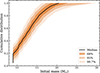 |
Fig. 7. Cumulative distributions of initial masses for the SN II progenitors in the sample derived from DBR models. |
In summary, accounting for the observed distribution of stellar velocities leads to systematically lower progenitor initial-mass estimates, but the effect remains modest compared to the statistical uncertainties. The SN II progenitor initial-mass distributions and the upper mass limit inferred from the sample are consistent with those obtained from non-rotating models.
6. Discussion
6.1. Low-luminosity progenitors
Evolutionary models of SN II progenitors generally predict final luminosities above log L ≃ 4.5 (Eldridge & Tout 2004; Poelarends et al. 2008; Woosley & Heger 2015; this work). However, a number of SN II progenitors have been observed at lower luminosities (log L ≃ 4.3−4.5). Given that the observed progenitor luminosities lie below the minimum final luminosities reached by our models, the inferred mass distributions accumulate at the minimum initial mass of the grid, explaining the distributions inferred for SNe 2008bk, 2009md, 2012A, 2022acko, and 2024afbl (see Sect. 4). This, in turn, indicates that a non-negligible fraction of SN II progenitors may populate the faint end of the luminosity distribution, which is not fully captured by current stellar evolution models.
The late evolutionary stages of stars close to the boundary between white-dwarf formation and SN explosions are particularly difficult to model. At solar metallicity, this transition occurs over a relatively narrow initial-mass range from 7 to 10 M⊙, where electron degeneracy and neutrino cooling play a dominant role in shaping the internal structure. These effects can lead to temperature inversions, off-centre shell ignition, and composition gradients, making the post-carbon-burning evolution particularly challenging to follow (see e.g. Miyaji et al. 1980; Nomoto et al. 1984; Poelarends et al. 2008; Woosley & Heger 2015; Limongi et al. 2024 for details).
In standard stellar evolution scenarios, stars in the initial-mass range of ∼7−10 M⊙ form ONe cores following carbon burning and subsequently enter a thermally pulsating phase. These objects are known as super-asymptotic giant branch stars, and their evolutionary outcome depends on the balance between ONe core growth and mass loss, resulting in either an ONe white dwarf or an ECSN. Stars with initial masses of ∼10−12 M⊙ ignite neon off-centre, while more massive stars ignite neon centrally; in both cases, the evolution ultimately leads to a CCSN. The exact mass limits remain uncertain, as they depend on the treatment of internal mixing, opacities, nuclear reaction rates, neutrino cooling, and numerical resolution, among other factors. In addition, these initial-mass limits vary with initial metallicity and rotational velocity.
For stars that do not undergo the second dredge-up, there is an increasing relation between initial mass and final luminosity. However, when the second dredge-up occurs, the convective envelope penetrates deeply into the interior efficiently dredging up the products of previous nuclear burning stages. This process precedes the onset of thermal pulses and results in a significant increase in the stellar luminosity, leading to values well above the minimum luminosity expected for CCSN progenitors (e.g. Poelarends et al. 2008; Fraser et al. 2011). Moreover, this leads to luminosities well above those inferred for some of the faintest observed SN II progenitors. Fraser et al. (2011) addressed the discrepancy between the low luminosities inferred for some SN II progenitors and predictions from stellar evolution models by proposing that stellar evolution proceeds sufficiently rapidly for the star to explode before the second dredge-up occurs. To achieve this, they increased the cross-section of the 12C + 12C reaction, motivated by the possible presence of a resonance (see Monpribat et al. 2022 for an updated discussion of this nuclear reaction). This approach allows progenitor models to reach luminosities as low as log L ≃ 4.3, thereby alleviating the tension between stellar evolution models and the observed luminosities of SN II progenitors. Overall, significant uncertainties remain in the late evolutionary stages of low-mass CCSN progenitors, and the ability of stellar evolution models to reproduce the faint end of the SN II progenitor population remains an open question.
6.2. The RSG problem
The first direct detection of a SN II progenitor was achieved more than two decades ago for SN 2003gd (Smartt et al. 2004). Since then, the number of identified SN II progenitors has steadily increased, with more than 20 progenitors now detected, along with a comparable number of upper limits on progenitor luminosities (see Van Dyk 2025 for a recent review). Early analyses of the SN II progenitor population based on direct progenitor detections suggested an upper initial-mass limit of ∼18 M⊙ (Smartt et al. 2009; Smartt 2015). This result appears to be in tension with stellar evolution models, which predict that more massive stars can retain substantial hydrogen-rich envelopes and thus produce SN II explosions, as well as with observations of more luminous – and therefore more massive – RSGs (Levesque et al. 2006). This absence of progenitors with initial masses above ∼25 M⊙ is commonly referred to as the ‘RSG problem’ (Smartt et al. 2009).
Davies & Beasor (2018) revised bolometric corrections and extinction estimates, finding an increased upper initial-mass limit of Mup = 19 M⊙, with a 95% upper confidence limit of < 27 M⊙, corresponding to a statistical significance of the RSG problem at the ∼2σ level; this result was later supported by Davies & Beasor (2020), who analysed the progenitor population directly in luminosity space, thereby avoiding uncertainties associated with converting luminosities into initial masses using stellar evolution models. Moreover, Beasor et al. (2025) analysed the impact of systematic uncertainties and found that, even the most luminous RSGs remain consistent with the observed SN II progenitor sample at the 3σ level. The reader is referred to Morozova et al. (2018) and Martinez et al. (2022) for estimates of the statistical significance of the RSG problem based on light-curve modelling, and to Fang et al. (2025) for estimates based on nebular spectral analyses.
Having determined the initial-mass distributions using both non-rotating and DBR models (Sect. 5), we next focused exclusively on the results from the DBR models. These results indicate that the upper initial-mass limit for SN II progenitors is Mup = 20.4 M⊙ (68% confidence), with a 95% upper confidence limit of 28.5 M⊙. This corresponds to a statistical significance of the RSG problem at the ∼2σ level. We note, however, that the stellar evolution models used in this analysis were computed assuming solar metallicity. Adopting specific metallicity values to each individual SN could lead to variations in the inferred masses. We emphasise that the analysis of the RSG problem constitutes an additional, exploratory analysis motivated by the availability of our results. The primary goal of this work is to compare the results obtained using non-rotating models and models computed with an observed distribution of initial rotational velocities.
6.3. SN II progenitors from mass gainers reaching critical rotation
In this work we have focused exclusively on the single evolutionary channel for SN II progenitors. However, it is well established that a large fraction of massive stars belong to binary systems (or higher-order multiples; Moe & Di Stefano 2017) and are expected to interact with a companion during their evolution (Sana et al. 2012).
In interacting binary systems, the initially more massive star transfers not only mass but also angular momentum to its companion. The accretion of angular momentum can strongly affect the rotational properties and the evolution of the secondary star, allowing mass gainers to approach critical rotation after accreting relatively small amounts of material (Packet 1981; Wang et al. 2020). Observationally, the distribution of rotational velocities of O- and B-type stars reveals a high-velocity tail, with projected velocities reaching up to ∼500 km s−1, commonly interpreted as the result of binary interaction (de Mink et al. 2013).
The accreted angular momentum spins up the outer layers of the secondary, and is subsequently transferred deeper into the star. As a consequence, by the end of the binary interaction phase, the mass gainer is more massive than initially and rotates nearly uniformly approaching the critical surface velocity. If this star subsequently undergoes advanced nuclear burning stages and retains a significant hydrogen-rich envelope at the end of its evolution, it may also explode as a SN II, thereby contributing to the observed SN II progenitor population. In the following, we incorporate this evolutionary channel into our analysis to provide a first-order estimate of its impact on our results.
We computed additional evolutionary models of single massive stars at solar metallicity, initially rotating uniformly at their critical surface velocity. The initial-mass range spans 9−16 M⊙ in steps of 1 M⊙. As discussed earlier, rotation enhances chemical mixing, producing more massive cores and, consequently, more luminous stars with stronger winds, which further reduce their hydrogen-rich envelopes. Therefore, models of more massive stars lose nearly all of their hydrogen-rich envelopes and therefore do not produce the SN type considered in this work.
To account for the mass-gainer evolutionary channel, we needed an estimate of the fraction of SNe II expected to originate from it. For this purpose, we adopted the results of Zapartas et al. (2019), who used binary population-synthesis simulations to estimate the fraction of SNe II arising from different evolutionary channels. They find that 55% of SN II progenitors originate from effectively single stars, i.e. stars that were born single or in very wide binary systems that do not experience binary interaction. In addition, about 14% of SN II progenitors originate from stars that have accreted mass through stable Roche-lobe overflow from a companion. The remaining fraction arises from various merger channels, which are not considered in the present study.
To assess the impact of the mass-gainer evolutionary channel, we used the progenitor of SN 2025pht as a case study. We performed an analysis analogous to that described in Sect. 3.3. First, we sampled progenitor luminosities from a Gaussian distribution (see Sect. 3.3). For 55% of the total MC trials, we assumed that the progenitors originate from the single-evolution channel and followed the same procedure as in the previous analysis using the DBR models. For 14% of the MC trials, we inferred the initial mass using the sampled luminosity and evolutionary models initially rotating at the critical surface velocity. Merger scenarios were not considered. We repeated this MC procedure 20 000 times.
As a result, we obtained the initial-mass distribution for the progenitor of SN 2025pht, including the contribution of the mass-gainer evolutionary channel, as shown in Fig. 8. We derive an initial mass of MZAMS = 13.7 M⊙. Although the inferred initial mass is lower than that obtained with the DBR models, a comparison with the non-rotating models shows that the median value remains consistent within 1σ.
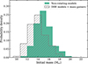 |
Fig. 8. Initial-mass distributions of the progenitor of SN 2025pht using non-rotating models (solid green bars) and DBR models including the contribution of mass gainers (dashed grey bars). |
This analysis provides a preliminary assessment of the impact of the mass-gainer evolutionary channel. We note, however, that the fraction of progenitors associated with each evolutionary channel is subject to uncertainties in stellar evolution modelling (see Zapartas et al. 2019). We also assumed that all mass gainers reach nearly uniform rotation at the critical surface velocity. Furthermore, in interacting binaries, mass transfer usually starts after the accreting star has already burned some fraction of its central hydrogen. In contrast, our critically rotating models start their evolution at the ZAMS. This temporal offset may affect the subsequent evolutionary phases. Overall, while highly simplified, the inclusion of a mass-gainer channel highlights the impact of binary interaction on the properties of SN II progenitors and on the interpretation of progenitor mass distributions.
6.4. Effect of metallicity on the progenitor initial-mass distribution
Metallicity is a fundamental parameter affecting stellar evolution and therefore the properties of SN progenitors. In the present study, however, we restricted our analysis to stellar models computed at solar metallicity. An important effect of metallicity is its influence on stellar wind mass-loss rates. Given that the winds of hot stars are line-driven, with radiative acceleration primarily provided by UV metal lines (e.g. C, N, O, and Fe-group elements), they are well known to depend on metallicity (e.g. Vink et al. 2001; Vink 2022). Such metallicity-driven differences in mass-loss behaviour directly affect the final properties of SN progenitors. By contrast, on the luminous and cool side of the HR diagram, recent studies provide no evidence of an explicit dependence of RSG mass loss on metallicity, although this remains under study (Antoniadis et al. 2025; van Loon 2025).
In massive stars, hydrogen burning proceeds predominantly via the CNO cycle. The cycle requires the presence of C, N, or O isotopes, which act as catalysts in the reaction network. Consequently, at lower metallicity, the initial abundance of these elements is reduced, which directly affects the energy generation of the CNO cycle. For a given density and temperature it will be lower than in the case of solar abundances. This leads to changes in the central temperature and density during hydrogen burning, ultimately affecting the main-sequence lifetime, core masses, and therefore the final luminosities (Mowlavi et al. 1998), which is the observable considered in this work.
The GENEVA and MIST grids of stellar evolution models at different initial metallicities show that, at fixed initial mass, the final stellar luminosity increases as the metallicity decreases (Ekström et al. 2012; Georgy et al. 2013; Choi et al. 2016; Eggenberger et al. 2021). In other words, if the progenitor of a SN II has a subsolar initial metallicity, adopting solar-metallicity models to construct the initial-mass distribution will result in an overestimation of its mass, while the opposite occurs for super-solar metallicities. This illustrates the impact of metallicity on the inferred progenitor masses. A more complete exploration of the parameter space, including variations in metallicity and rotation, will be considered in future work.
7. Conclusions
In this work we quantified the differences in the inferred initial masses of SN II progenitors with pre-explosion detections when using non-rotating evolutionary models (a common approach in the literature) compared to rotating models in which the initial rotational velocities were drawn from the observed distribution of massive stars. We compared the progenitor initial masses for each SN, statistical distributions of the initial masses, and the upper initial-mass limit derived using the two approaches. In all cases, we find that the differences are small, and the values obtained with non-rotating models are consistent with those derived from DBR models.
Using the observed distribution of initial rotational velocities for SN II progenitors, we revisited the upper initial-mass limit inferred from pre-explosion imaging. We obtained Mup = 20.4 M⊙, with a 95% upper confidence limit of 28.5 M⊙, which places the statistical significance of the RSG problem within the 2σ level, in agreement with recent studies (Davies & Beasor 2020; Beasor et al. 2025).
Our analyses indicate that, although rotation affects the evolutionary tracks of massive stars, its impact on progenitor mass estimates from pre-SN imaging remains modest within the current uncertainties when the observed distribution of initial rotational velocities is taken into account. Therefore, we conclude that explicitly incorporating this distribution is not necessary to obtain significantly more precise estimates of progenitor initial masses. These results offer a useful reference for future studies and suggest that non-rotating models remain sufficient for estimating SN II progenitor masses, at least within the current observational limits.
Data availability
The tables containing the stellar properties at core carbon depletion for the full grid of models, along with the MESA input files used in this work, are publicly available at https://doi.org/10.5281/zenodo.19099684.
Acknowledgments
We thank the referee for a careful reading of the manuscript and for constructive comments that helped improve this work. L.M. acknowledges support from a CONICET postdoctoral fellowship. Software: MESA (Paxton et al. 2011, 2013, 2015, 2018, 2019; Jermyn et al. 2023), NumPy (Oliphant 2006; Van Der Walt et al. 2011), matplotlib (Hunter 2007), SciPy (Virtanen et al. 2020), pandas (McKinney 2010), jupyter (Kluyver et al. 2016).
References
- Antoniadis, K., Zapartas, E., Bonanos, A. Z., et al. 2025, A&A, 702, A178 [NASA ADS] [CrossRef] [EDP Sciences] [Google Scholar]
- Asplund, M., Amarsi, A. M., & Grevesse, N. 2021, A&A, 653, A141 [NASA ADS] [CrossRef] [EDP Sciences] [Google Scholar]
- Beasor, E. R., Smith, N., & Jencson, J. E. 2025, ApJ, 979, 117 [Google Scholar]
- Björklund, R., Sundqvist, J. O., Singh, S. M., Puls, J., & Najarro, F. 2023, A&A, 676, A109 [NASA ADS] [CrossRef] [EDP Sciences] [Google Scholar]
- Chieffi, A., & Limongi, M. 2013, ApJ, 764, 21 [Google Scholar]
- Choi, J., Dotter, A., Conroy, C., et al. 2016, ApJ, 823, 102 [Google Scholar]
- Davies, B., & Beasor, E. R. 2018, MNRAS, 474, 2116 [NASA ADS] [CrossRef] [Google Scholar]
- Davies, B., & Beasor, E. R. 2020, MNRAS, 493, 468 [NASA ADS] [CrossRef] [Google Scholar]
- de Mink, S. E., Langer, N., Izzard, R. G., Sana, H., & de Koter, A. 2013, ApJ, 764, 166 [Google Scholar]
- Eggenberger, P., Ekström, S., Georgy, C., et al. 2021, A&A, 652, A137 [NASA ADS] [CrossRef] [EDP Sciences] [Google Scholar]
- Ekström, S., Georgy, C., Eggenberger, P., et al. 2012, A&A, 537, A146 [Google Scholar]
- Eldridge, J. J., & Tout, C. A. 2004, MNRAS, 353, 87 [NASA ADS] [CrossRef] [Google Scholar]
- Eldridge, J. J., Izzard, R. G., & Tout, C. A. 2008, MNRAS, 384, 1109 [Google Scholar]
- Eldridge, J. J., Guo, N. Y., Rodrigues, N., Stanway, E. R., & Xiao, L. 2019, PASA, 36, e041 [NASA ADS] [CrossRef] [Google Scholar]
- Endal, A. S., & Sofia, S. 1978, ApJ, 220, 279 [NASA ADS] [CrossRef] [Google Scholar]
- Fang, Q., Moriya, T. J., & Maeda, K. 2025, ApJ, 986, 39 [Google Scholar]
- Farmer, R., Fields, C. E., Petermann, I., et al. 2016, ApJS, 227, 22 [NASA ADS] [CrossRef] [Google Scholar]
- Filippenko, A. V., Matheson, T., & Ho, L. C. 1993, ApJ, 415, L103 [NASA ADS] [CrossRef] [Google Scholar]
- Fraser, M., Ergon, M., Eldridge, J. J., et al. 2011, MNRAS, 417, 1417 [NASA ADS] [CrossRef] [Google Scholar]
- Georgy, C., Ekström, S., Eggenberger, P., et al. 2013, A&A, 558, A103 [NASA ADS] [CrossRef] [EDP Sciences] [Google Scholar]
- Goldman, S. R., van Loon, J. T., Zijlstra, A. A., et al. 2017, MNRAS, 465, 403 [Google Scholar]
- Heger, A., Langer, N., & Woosley, S. E. 2000, ApJ, 528, 368 [NASA ADS] [CrossRef] [Google Scholar]
- Heger, A., Woosley, S. E., & Spruit, H. C. 2005, ApJ, 626, 350 [Google Scholar]
- Hellinger, E. 1909, J. Reine Angew. Math., 1909, 210 [CrossRef] [Google Scholar]
- Hiramatsu, D., Howell, D. A., Van Dyk, S. D., et al. 2021, Nat. Astron., 5, 903 [NASA ADS] [CrossRef] [Google Scholar]
- Holgado, G., Simón-Díaz, S., Herrero, A., & Barbá, R. H. 2022, A&A, 665, A150 [NASA ADS] [CrossRef] [EDP Sciences] [Google Scholar]
- Huang, W., Gies, D. R., & McSwain, M. V. 2010, ApJ, 722, 605 [Google Scholar]
- Hunter, J. D. 2007, Comput. Sci. Eng., 9, 90 [NASA ADS] [CrossRef] [Google Scholar]
- Jerkstrand, A., Smartt, S. J., Sollerman, J., et al. 2015, MNRAS, 448, 2482 [Google Scholar]
- Jermyn, A. S., Bauer, E. B., Schwab, J., et al. 2023, ApJS, 265, 15 [NASA ADS] [CrossRef] [Google Scholar]
- Kilpatrick, C. D., Izzo, L., Bentley, R. O., et al. 2023, MNRAS, 524, 2161 [Google Scholar]
- Kilpatrick, C. D., Suresh, A., Davis, K. W., et al. 2025, ApJ, 992, L10 [Google Scholar]
- Kippenhahn, R., Ruschenplatt, G., & Thomas, H.-C. 1980, A&A, 91, 175 [NASA ADS] [Google Scholar]
- Kippenhahn, R., Weigert, A., & Weiss, A. 2013, Stellar Structure and Evolution (Springer) [Google Scholar]
- Kluyver, T., Ragan-Kelley, B., Pérez, F., et al. 2016, Positioning and Power in Academic Publishing: Players, Agents and Agendas (IOS Press), 87 [Google Scholar]
- Langer, N. 2012, ARA&A, 50, 107 [CrossRef] [Google Scholar]
- Langer, N., Fricke, K. J., & Sugimoto, D. 1983, A&A, 126, 207 [NASA ADS] [Google Scholar]
- Levesque, E. M., Massey, P., Olsen, K. A. G., et al. 2006, ApJ, 645, 1102 [NASA ADS] [CrossRef] [Google Scholar]
- Li, Y., Chen, X.-H., & Chen, H.-L. 2019, ApJ, 870, 77 [NASA ADS] [CrossRef] [Google Scholar]
- Limongi, M., Roberti, L., Chieffi, A., & Nomoto, K. 2024, ApJS, 270, 29 [NASA ADS] [CrossRef] [Google Scholar]
- Lucy, L. B. 1974, AJ, 79, 745 [Google Scholar]
- Luo, J., Zhang, L., Chen, B.-Q., et al. 2025, ApJ, 982, L55 [Google Scholar]
- Maeder, A. 2009, Physics, Formation and Evolution of Rotating Stars (Springer) [Google Scholar]
- Maeder, A., & Meynet, G. 2000, ARA&A, 38, 143 [Google Scholar]
- Martinez, L., Bersten, M. C., Anderson, J. P., et al. 2020, A&A, 642, A143 [NASA ADS] [CrossRef] [EDP Sciences] [Google Scholar]
- Martinez, L., Bersten, M. C., Anderson, J. P., et al. 2022, A&A, 660, A41 [NASA ADS] [CrossRef] [EDP Sciences] [Google Scholar]
- Martins, F., & Palacios, A. 2013, A&A, 560, A16 [NASA ADS] [CrossRef] [EDP Sciences] [Google Scholar]
- Maund, J. R. 2017, MNRAS, 469, 2202 [NASA ADS] [CrossRef] [Google Scholar]
- McKinney, W. 2010, in Proceedings of the 9th Python in Science Conference, eds. S. van der Walt, & J. Millman, 56 [Google Scholar]
- Meynet, G., & Maeder, A. 2000, A&A, 361, 101 [NASA ADS] [Google Scholar]
- Minkowski, R. 1941, PASP, 53, 224 [NASA ADS] [CrossRef] [Google Scholar]
- Miyaji, S., Nomoto, K., Yokoi, K., & Sugimoto, D. 1980, PASJ, 32, 303 [Google Scholar]
- Moe, M., & Di Stefano, R. 2017, ApJS, 230, 15 [Google Scholar]
- Monpribat, E., Martinet, S., Courtin, S., et al. 2022, A&A, 660, A47 [CrossRef] [EDP Sciences] [Google Scholar]
- Morozova, V., Piro, A. L., & Valenti, S. 2018, ApJ, 858, 15 [Google Scholar]
- Mowlavi, N., Meynet, G., Maeder, A., Schaerer, D., & Charbonnel, C. 1998, A&A, 335, 573 [NASA ADS] [Google Scholar]
- Nomoto, K., Thielemann, F. K., & Yokoi, K. 1984, ApJ, 286, 644 [Google Scholar]
- Oliphant, T. E. 2006, A guide to NumPy (USA: Trelgol Publishing), 1 [Google Scholar]
- O’Neill, D., Kotak, R., Fraser, M., et al. 2019, A&A, 622, L1 [NASA ADS] [CrossRef] [EDP Sciences] [Google Scholar]
- Packet, W. 1981, A&A, 102, 17 [NASA ADS] [Google Scholar]
- Paxton, B., Bildsten, L., Dotter, A., et al. 2011, ApJS, 192, 3 [Google Scholar]
- Paxton, B., Cantiello, M., Arras, P., et al. 2013, ApJS, 208, 4 [Google Scholar]
- Paxton, B., Marchant, P., Schwab, J., et al. 2015, ApJS, 220, 15 [Google Scholar]
- Paxton, B., Schwab, J., Bauer, E. B., et al. 2018, ApJS, 234, 34 [NASA ADS] [CrossRef] [Google Scholar]
- Paxton, B., Smolec, R., Schwab, J., et al. 2019, ApJS, 243, 10 [Google Scholar]
- Pessi, T., Desai, D. D., Prieto, J. L., et al. 2025, A&A, 703, A34 [NASA ADS] [CrossRef] [EDP Sciences] [Google Scholar]
- Poelarends, A. J. T., Herwig, F., Langer, N., & Heger, A. 2008, ApJ, 675, 614 [Google Scholar]
- Sana, H., de Mink, S. E., de Koter, A., et al. 2012, Science, 337, 444 [Google Scholar]
- Shivvers, I., Modjaz, M., Zheng, W., et al. 2017, PASP, 129, 054201 [NASA ADS] [CrossRef] [Google Scholar]
- Smartt, S. J. 2015, PASA, 32, e016 [NASA ADS] [CrossRef] [Google Scholar]
- Smartt, S. J., Maund, J. R., Hendry, M. A., et al. 2004, Science, 303, 499 [NASA ADS] [CrossRef] [Google Scholar]
- Smartt, S. J., Eldridge, J. J., Crockett, R. M., & Maund, J. R. 2009, MNRAS, 395, 1409 [CrossRef] [Google Scholar]
- Spruit, H. C. 2002, A&A, 381, 923 [CrossRef] [EDP Sciences] [Google Scholar]
- Straniero, O., Dominguez, I., Piersanti, L., Giannotti, M., & Mirizzi, A. 2019, ApJ, 881, 158 [NASA ADS] [CrossRef] [Google Scholar]
- Takáts, K., Pignata, G., Pumo, M. L., et al. 2015, MNRAS, 450, 3137 [CrossRef] [Google Scholar]
- Van Der Walt, S., Colbert, S. C., & Varoquaux, G. 2011, Comput. Sci. Eng., 13, 22 [Google Scholar]
- Van Dyk, S. D. 2025, Galaxies, 13, 33 [Google Scholar]
- Van Dyk, S. D., Zheng, W., Maund, J. R., et al. 2019, ApJ, 875, 136 [Google Scholar]
- Van Dyk, S. D., Bostroem, K. A., Zheng, W., et al. 2023, MNRAS, 524, 2186 [Google Scholar]
- Van Dyk, S. D., Srinivasan, S., Andrews, J. E., et al. 2024, ApJ, 968, 27 [NASA ADS] [CrossRef] [Google Scholar]
- van Loon, J. T. 2025, Galaxies, 13, 72 [Google Scholar]
- Vink, J. S. 2022, ARA&A, 60, 203 [NASA ADS] [CrossRef] [Google Scholar]
- Vink, J. S., de Koter, A., & Lamers, H. J. G. L. M. 2001, A&A, 369, 574 [NASA ADS] [CrossRef] [EDP Sciences] [Google Scholar]
- Virtanen, P., Gommers, R., Oliphant, T. E., et al. 2020, Nat. Methods, 17, 261 [Google Scholar]
- Wang, C., Langer, N., Schootemeijer, A., et al. 2020, ApJ, 888, L12 [NASA ADS] [CrossRef] [Google Scholar]
- Wen, J., Yang, M., Gao, J., et al. 2024, ApJS, 275, 33 [Google Scholar]
- Williams, B. F., Hillis, T. J., Murphy, J. W., et al. 2018, ApJ, 860, 39 [NASA ADS] [CrossRef] [Google Scholar]
- Woosley, S. E., & Heger, A. 2007, Phys. Rep., 442, 269 [Google Scholar]
- Woosley, S. E., & Heger, A. 2015, ApJ, 810, 34 [NASA ADS] [CrossRef] [Google Scholar]
- Xiang, D., Mo, J., Wang, X., et al. 2024, ApJ, 969, L15 [Google Scholar]
- Zahn, J. P. 1992, A&A, 265, 115 [NASA ADS] [Google Scholar]
- Zapartas, E., de Mink, S. E., Justham, S., et al. 2019, A&A, 631, A5 [NASA ADS] [CrossRef] [EDP Sciences] [Google Scholar]
We use ‘SNe II’ to refer to hydrogen-rich CCSNe, excluding type IIb, IIn, and SN 1987A-like events.
We note that our simulations are stopped at the end of core carbon burning. For the lowest-mass models, we continued the evolutionary calculations in order to determine whether neon ignition occurs and thus assess the final fate of the star.
For non-rotating models, the use of the cKDTree algorithm is unnecessary, as linear interpolation is sufficient.
Appendix A: Hertzsprung–Russell diagrams
Figure A.1 shows HR diagrams for a subsample of stellar models.
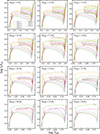 |
Fig. A.1. HR diagrams for stellar evolutionary models. Each panel corresponds to a fixed initial mass, as indicated in the panel labels. For a given mass, evolutionary tracks computed with different initial rotational velocities are shown. Only a subset of the models is shown, for visualisation purposes. |
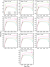 |
Fig. A.1. continued. |
Appendix B: Additional progenitor mass distribution diagrams
Figure B.1 shows the initial-mass distributions for the complete sample of SN II progenitors, obtained from non-rotating and DBR models. Additionally, Fig. B.2 shows the CDF of the initial mass for the SNe II in the sample, derived from non-rotating models.
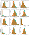 |
Fig. B.1. Initial-mass distributions of SN II progenitors in the sample from non-rotating (green) and DBR models (orange). |
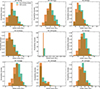 |
Fig. B.1. continued. |
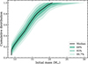 |
Fig. B.2. Cumulative distributions of initial masses for the SN II progenitors in the sample derived from non-rotating models. |
All Tables
Maximum initial mass across the computed grids for different initial surface velocities.
Progenitor initial masses from non-rotating and DBR models for each SN II in the sample.
All Figures
|
Fig. 1. HR diagrams for a subsample of stellar models. Left panel: Non-rotating models. Coloured lines correspond to models with initial masses of 10, 15, 20, and 25 M⊙, and the remaining models are shown as faint grey lines. Right panel: Evolutionary tracks for stars with initial masses of 10, 15, 20, and 25 M⊙ and different initial rotational velocities, as indicated in the panel label. We note that the model with an initial mass of 25 M⊙ and an initial rotational velocity of 400 km s−1 lies outside the parameter space of the current study (see Table 2). |
| In the text | |
|
Fig. 2. Stellar luminosities at core carbon depletion for a range of initial masses and surface velocities. Only a subset of the models is shown, for visualisation purposes. |
| In the text | |
|
Fig. 3. Probability density of rotational velocities. Projected rotational velocities of young Galactic O-type stars from Holgado et al. (2022) with masses below 32 M⊙ are shown as a histogram. The deconvolved distribution, obtained using the method of Lucy (1974), is overplotted as a thick line. |
| In the text | |
|
Fig. 4. Initial-mass distribution of the progenitor of SN 2025pht using the DBR models. The solid vertical line corresponds to the median of the distribution, and dashed vertical lines are the 16th and 84th percentiles. |
| In the text | |
|
Fig. 5. Median of the initial-mass distribution of SN II progenitors in the sample, derived from non-rotating (green dots) and DBR models (orange triangles). Error bars correspond to the 16th and 84th percentiles. |
| In the text | |
|
Fig. 6. PDFs of the SN II progenitor’s initial mass, derived from non-rotating (dashed green line) and DBR models (solid orange line). |
| In the text | |
|
Fig. 7. Cumulative distributions of initial masses for the SN II progenitors in the sample derived from DBR models. |
| In the text | |
|
Fig. 8. Initial-mass distributions of the progenitor of SN 2025pht using non-rotating models (solid green bars) and DBR models including the contribution of mass gainers (dashed grey bars). |
| In the text | |
|
Fig. A.1. HR diagrams for stellar evolutionary models. Each panel corresponds to a fixed initial mass, as indicated in the panel labels. For a given mass, evolutionary tracks computed with different initial rotational velocities are shown. Only a subset of the models is shown, for visualisation purposes. |
| In the text | |
|
Fig. A.1. continued. |
| In the text | |
|
Fig. B.1. Initial-mass distributions of SN II progenitors in the sample from non-rotating (green) and DBR models (orange). |
| In the text | |
|
Fig. B.1. continued. |
| In the text | |
|
Fig. B.2. Cumulative distributions of initial masses for the SN II progenitors in the sample derived from non-rotating models. |
| In the text | |
Current usage metrics show cumulative count of Article Views (full-text article views including HTML views, PDF and ePub downloads, according to the available data) and Abstracts Views on Vision4Press platform.
Data correspond to usage on the plateform after 2015. The current usage metrics is available 48-96 hours after online publication and is updated daily on week days.
Initial download of the metrics may take a while.