| Issue |
A&A
Volume 710, June 2026
|
|
|---|---|---|
| Article Number | A74 | |
| Number of page(s) | 9 | |
| Section | Stellar structure and evolution | |
| DOI | https://doi.org/10.1051/0004-6361/202557331 | |
| Published online | 03 June 2026 | |
GeV emission in the region of Vela: A new view of the supernova remnant
1
Escuela de Física, Universidad de Costa Rica, Montes de Oca, San José, 11501-2060, Costa Rica
2
ECCI/CITIC, Universidad de Costa Rica, Montes de Oca, San José, 11501-2060, Costa Rica
★ Corresponding author: This email address is being protected from spambots. You need JavaScript enabled to view it.
Received:
19
September
2025
Accepted:
16
April
2026
Abstract
Context. The Vela supernova remnant (SNR), G263.9 − 3.3, and its pulsar wind nebula (PWN), Vela X, is one of the closest such systems, and it has been studied using observations across the electromagnetic spectrum. The SNRs are known sources of gamma rays with energies from the GeV to TeV range. In the GeV band, a cluster of catalogued unidentified Fermi-LAT point sources are found across the large angular extension of the Vela SNR.
Aims. We aim to search for a high-energy signature associated with the SNR.
Methods. We applied two independent machine-learning algorithms to classify unidentified point sources in the Vela region by comparing their properties to those of known populations of Fermi pulsars and active galactic nuclei. We analysed LAT data and modelled the spectrum of any emission attributable to Vela using leptonic and hadronic processes typical of SNRs.
Results. We find that most of the ‘point sources’ catalogued within the extent of Vela do not share characteristics with those of the two most common Fermi point-like source populations and that even after the emission attributed to these point sources is subtracted, considerable residual emission is seen throughout Vela. Morphologically, most of the GeV emission is found within the shell of the SNR. We conclude that the majority of the catalogued point sources are likely spurious, and the GeV gamma rays come from an extended source, which we argue is the counterpart of the Vela SNR. Adopting a simple morphology given by a uniform disk for the emission, the resulting extension is ∼6.5°. The northeastern portion of G263.9 − 3.3, where the ambient density is thought to be higher, is brighter in gamma rays than the southern and western regions. The spectrum of the emission is best fit with a hadronic model. These facts make the hadronic origin of the gamma rays more likely.
Key words: pulsars: general / ISM: supernova remnants / gamma rays: general
© The Authors 2026
 Open Access article, published by EDP Sciences, under the terms of the Creative Commons Attribution License (https://creativecommons.org/licenses/by/4.0), which permits unrestricted use, distribution, and reproduction in any medium, provided the original work is properly cited.
This article is published in open access under the Subscribe to Open model. This email address is being protected from spambots. You need JavaScript enabled to view it. to support open access publication.
1. Introduction
Supernova remnants (SNR) have been considered for many years plausible sources of Galactic cosmic rays. Particles gain energy and become relativistic in the shocks of SNRs, resulting in distinctive signatures such as synchrotron emission from radio to X-rays and gamma-ray emission from inverse Compton scattering and non-thermal Bremsstrahlung (leptonic origin) or neutral pion decay (hadronic origin). The Large Area Telescope (LAT) onboard the Fermi satellite has been observing the sky since 2008, detecting photons with energies from ∼20 MeV to more than 300 GeV (Atwood et al. 2009). The LAT fourth source catalogue (4FGL) contains 7194 gamma-ray sources (Abdollahi et al. 2020; Ballet et al. 2023), including a growing number of SNRs.
The Vela SNR, G263.9 − 3.3, 8° diameter, is one of the most studied and closest SNRs to Earth. It is a typical example of a middle-aged composite SNR, which harbours the Vela X pulsar wind nebula (PWN) produced by the energetic Vela pulsar, PSR B0833 − 45. This pulsar has a characteristic age τC = 11 kyr, a spin period of P = 89 ms and a spin-down power Ė = 6.9 × 1036 erg s−1. Its distance, ∼290 pc, has been measured by parallax (Caraveo et al. 2001; Dodson et al. 2003). A shock radius of 20 pc, shock velocities of 660 − 1020 km s−1 and an age of (7 − 12) kyr have also been estimated (Sushch & Hnatyk 2014).
Radio observations of Vela reveal a prominent 2° ×3° region in the centre, dubbed Vela X. This is a synchrotron nebula likely produced by the pulsar (e.g. Frail et al. 1997). Another radio region seen within Vela, originally designated as Vela Z, is associated with a different SNR, Vela Junior (G266.2 − 1.2). Alvarez et al. (2001) measured the integrated flux densities between 30 and 8400 MHz (Sν) of these two regions, as well as those of Vela Y, which corresponds to the northern shell of the Vela SNR. The radio spectral index of Vela Y is α ∼ −0.70 (Sν ∝ να). Using HI observations, Dubner et al. (1998) estimated an ambient atomic density of 1 − 2 cm−3 and an initial explosion kinetic energy of (1 − 2.5)×1051 erg for the Vela SNR. They found evidence of atomic hydrogen located around the SNR, with denser emission in the north and east. Sushch et al. (2011) explained the observed NE-SW asymmetry of the SNR. In their model, the wind from a nearby Wolf-Rayet star causes the NE part of the SNR to expand into a medium with an average density of shock-evaporated clouds that is about four times higher than that in the SW part (nucleon number densities 0.4 and 0.1 cm−3, respectively). In this model, the required kinetic energy in the supernova explosion is 0.14 × 1051 erg. Regarding the high-energy particle content, Sushch & Hnatyk (2014) proposed a scenario in which the multiple shocks seen inside the remnant lead to a uniform distribution of relativistic particles in the interior.
The Vela SNR is a bright source of X-rays (see Lu & Aschenbach 2000, and references therein). The NE appears brighter and less extended than the SW part of the SNR. Aschenbach et al. (1995) discovered several bow-shaped X-ray features outside the blast-wave front with the ROSAT telescope (the so-called Vela ‘shrapnels’), which are likely dense ejecta fragments overtaking the main blast wave. Evidence for expansion in a clumpy medium has also been found in the NE, with clump densities of 0.5 − 1 cm−3 (Bocchino et al. 1999). Embedded within the radio PWN, an X-ray feature known as the ‘cocoon’ is seen (Markwardt & Ögelman 1997), likely produced by high-energy electrons from the pulsar. This elongated synchrotron structure has an extension of ∼1.5°, with harder emission concentrated near the pulsar (Slane et al. 2018). More recently, Mayer et al. (2023) performed a detailed study of Vela X-ray emission with the eROSITA telescope, revealing an SNR with complex morphology and an extent of 10° ×8°. Interestingly, they discovered an extended synchrotron nebula around Vela X, elongated in the north-south direction with a diameter of ∼5°. This nebula could be produced by relatively recent injection from the pulsar after the ‘crushing’ of the old nebula by the reverse shock, or by efficient diffusion of high-energy particles from Vela X. Vela could thus be an example of a system where particles from the pulsar are trapped within the turbulent environment of the SNR, a possible explanation for the so-called TeV halos (Fang et al. 2019). Indeed, Huang et al. (2018) showed that the diffusion of electrons that have escaped from Vela X has to be suppressed given the flux of cosmic ray electrons seen on Earth.
Emission from Vela X has also been detected at gamma-ray energies. The Fermi-LAT found the GeV counterpart to the radio nebula (Abdo et al. 2010b; Grondin et al. 2013) and the High Energy Stereoscopic System (H.E.S.S.) found TeV emission in a region that encompasses the X-ray cocoon, although it is somewhat more extended (Aharonian et al. 2006). The Vela pulsar itself is also a very bright GeV source (Abdo et al. 2010a). Tibaldo et al. (2018) found that the LAT emission from Vela X is made up of two components. Below 100 GeV the emission has a soft spectrum with spectral index ∼2.2 and extends over a region consistent with the radio nebula. Above 100 GeV the spectral index is ∼0.9 and this hard emission comes from a smaller region coinciding with the X-ray cocoon. The spectrum of the hard component connects smoothly to that measured by H.E.S.S. at TeV energies. A more recent analysis by Lange et al. (2025) including lower energy events and removing the pulsed emission from PSR B0833 − 45 produced somewhat different results compared to those of Tibaldo et al. (2018). They concluded that two extended sources with similar spectral indices of 2.33 constitute a more adequate description of Vela X. The larger source encompasses most of the known radio emission from Vela X and shows evidence of spectral hardening at the highest energies (> 100 GeV) and the smaller source located to the NW of Vela X is only detected below 100 GeV. Given their similar spectral indices, the authors point out that the smaller source could be related to the PWN; however, an origin in the SNR or in an interaction of the PWN with SNR ejecta cannot be ruled out.
Regarding other GeV sources in the Vela region, there are 35 point sources without known association in the latest 4FGL catalogue (4FGL-DR4, Abdollahi et al. 2022; Ballet et al. 2023) located within 4.5° of the coordinates RA = 129.6°, Dec = −45.3° near the centre of the SNR. Most of these sources are seen in the direction of the NE shell of Vela. We note that within 8° of these coordinates, there are five additional unassociated sources along the Galactic plane ∼3° from the SE shell of Vela, and four more at a similar angular distance to the south. A recent search for extended LAT sources in the Galactic plane found a candidate with a radius of 2.85° (68% containment assuming a 2D Gaussian morphology) and a centre located within the extent of Vela X (Abdollahi et al. 2024). This source was potentially associated with the Vela pulsar; however, a cautious interpretation of this result was given in that work, as the actual morphology of the source is likely not well represented by the assumed 2D Gaussian model. Abdollahi et al. (2024) also pointed out that a considerable 39% change in the TS source extension (a measurement of the source significance; see below) was observed when alternative models were adopted for the interstellar diffuse emission.
Unidentified LAT point sources that are clustered together could be related to a single object (Cozzolongo et al. 2025). Further evidence to confirm this may come from detecting an extended source, such as an SNR or a PWN in other bands of the electromagnetic spectrum (e.g. Araya 2018, 2020). In this work we analysed LAT data in Section 2 to search for an extended GeV source in the region of Vela and to test its possible association with the SNR and/or PWN system. We adopted a classification procedure (explained in Section 2.2) to decide which of the 4FGL point sources of unknown nature could in fact be part of Vela, and we present simple models that can explain the origin of the gamma rays in the SNR in Section 3.
2. LAT data
We analysed publicly available LAT data1 collected between August 16, 2008 and June 20, 2025, corresponding to mission elapsed times (MET) 240623858 s to 772148810 s, in a 20° ×20° region of interest (RoI) around the coordinates RA, Dec = (129.6° , − 45.3° ) with the fermitools2 version 2.5.1 through the fermipy package version 1.4.0 (Wood et al. 2017). Since the Vela pulsar is a very bright source of gamma rays we used an updated pulsar ephemeris solution3 valid in the same time range to assign pulse phases to the events using the Tempo2 software (Hobbs et al. 2006). We defined the intervals of the off-pulse phase window 0 − 0.1 and 0.7 − 1 and removed events in the on-pulse window for the entire analysis. We set the fermipy parameter expscale=0.4 which corrects the exposure due to our phase selection. We selected events with energies above 1 GeV for improved angular resolution to carry out a morphological study and used the energy range 0.1 − 100 GeV to extract the source spectrum. Since the PWN Vela X shows an additional high-energy component that is detected with the LAT above 100 GeV, we set this value as the upper energy range. For the spectral and morphological analyses we selected front- and back-converted SOURCE class events (with the parameters evclass=128, evtype=3). To avoid contamination from the Earth’s limb, the maximum zenith angle was set to 105° for the morphological study using events with energies above 1 GeV, and to 90° for the spectral analysis including lower energies. We binned the data with a spatial scale of 0.05° per pixel and ten bins per decade in energy for exposure calculations. We used the appropriate response functions for this data set, P8R3_SOURCE_V3, and applied the maximum likelihood technique (Mattox et al. 1996) to model the data. The model of a source is convolved with the response functions to predict the number of counts in the spatial and energy bins. A fit of the free parameters maximizes the probability that the model will explain the data in each bin. The detection significance of a new source that has one additional free parameter, for example, can be calculated as the square root of the test statistic (TS), defined as TS = −2 log (ℒ0/ℒ), with ℒ and ℒ0 the maximum likelihood functions for a model with the new source and for the model without this additional source (the null hypothesis), respectively. Our starting model for the gamma-ray emission in the region included sources found in the 4FGL-DR4 catalogue. The diffuse Galactic emission is described by the file gll_iem_v07.fits and the isotropic emission and the residual cosmic-ray background are given by iso_P8R3_SOURCE_V3_v1.txt, both provided with the fermitools. The energy dispersion correction was applied to all sources except for the isotropic component.
2.1. Previously studied LAT sources in the region
From the unassociated sources in the region of Vela, we considered the source 4FGL J0822.8 − 4207 to be plausibly associated with the SNR Puppis A (Araya et al. 2022; Giuffrida et al. 2025) and replaced its point-like model with a small disk as found by Giuffrida et al. (2025). The source PS J0824.0 − 4329, located to the south of Puppis A and proposed by Giuffrida et al. (2025) to better account for the emission in this region, was included in the model. Furthermore, these authors used a different template to describe the emission from Puppis A compared to the one in the catalogue, which is not sufficient to explain the emission to the west of Puppis A. Therefore, we included two additional point sources in the model to account for this emission and optimized their locations with our data, resulting in the coordinates (RA, Dec) = (125.07°, −42.89°) and (RA, Dec) = (125.46°, −43.21°). Additionally, we adopted the model obtained by Lange et al. (2025) to describe the emission from Vela X with two geometrical templates consisting of a Gaussian and a disk to replace the source 4FGL J0834.3 − 4542e. Finally, according to Peron et al. (2024), several stellar clusters in the Vela molecular cloud ridge are sources of gamma rays. These sources correspond to the unassociated sources 4FGL J0844.9 − 4117, 4FGL J0859.3 − 4342, 4FGL J0900.2 − 4608, 4FGL J0857.7 − 4256c, which we kept in the model. We also adopted their extended sources to model the emission from RCW 27 (replacing the point source 4FGL J0838.4 − 3952, located ∼5.4° away from the centre of the RoI), RCW 38 (replacing 4FGL J0859.2 − 4729, see also Ge et al. 2024) and an additional source, which they labeled ‘gas core’, replacing 4FGL J0900.5 − 4434c and 4FGL J0901.1 − 4456c. Since G264.681 + 00.272 and G264.220 + 00.216 are classified as candidate HII regions (Anderson et al. 2014) we did not consider their association to 4FGL J0853.1 − 4407 to be firmly established. This leaves 26 point sources of unknown nature within 4.5° from the centre of the analysis region, most of which are located within the extent of the Vela SNR shell. We found that even after subtracting the emission from these sources, considerable residual emission is seen across the shell of Vela, but a more adequate study of the SNR features at GeV energies requires deciding which unidentified point sources could be related to it. In order to know which of these sources could potentially be associated with independent objects and thus should be kept in the model, we performed two classification schemes described in the following section.
2.2. Source classification
In the original 4FGL release (Abdollahi et al. 2020) most of the identified or associated point sources (∼63%) correspond to blazars, an extreme type of active galactic nuclei (AGN). Based on their optical properties, these AGN can be classified into BL Lacertae objects (BLLs) and flat spectrum radio quasars (FSRQs). The second most common class of identified or associated point sources corresponds to pulsars. AGN and pulsars show distinct spectral features in the 4FGL catalogue (Abdollahi et al. 2020). Around 27% of the catalogued point sources do not have a known counterpart at other wavelengths.
Machine learning provides adequate classification and characterization of point-like LAT sources (see, e.g. Saz Parkinson et al. 2016; Xiao et al. 2020; Chiaro et al. 2021; Finke et al. 2021; Bhat & Malyshev 2022; Zhu et al. 2023). We adopted two pipelines to classify sources of unknown nature based on their gamma-ray properties: (i) a multi-class neural network4 that decides whether a source is an AGN or not, and (ii) a calibrated support vector machine (SVM) ensemble that separates pulsar-like from non-pulsar-like sources to flag pulsar candidates. Both models were trained on the spectral and variability parameters of the 4FGL-DR4 catalogue and return a probability that a given source belongs to any of the classes. For training, we used sources with a designation in the 4FGL CLASS1 column (meaning that a source is identified or likely to belong to a certain class of objects). Unassociated 4FGL sources with an empty CLASS1 entry were treated as unidentified objects to be classified and were not used as labelled training examples. Finally, we cross-checked the results obtained in methods (i) and (ii) for consistency.
2.2.1. AGN candidate selection
For the AGN classifier we only kept sources with CLASS1 = BLL or FSRQ as positive examples, and we grouped all other known classes that are not AGN (pulsars of any type, pulsar wind nebulae, supernova remnants, globular clusters, star-forming regions, X-ray and/or γ-ray binaries, novae, normal or starburst galaxies) into a single nonAGN label. Blazar candidates of uncertain type (BCU) and AGN subclasses that are neither BLL nor FSRQ were excluded from the training set and were only used later as independent test samples. The 4FGL AGN subclasses other than BLL, FSRQ, and BCU constitute less than ∼2% of AGN and can be neglected. This choice follows common LAT source classification practice where blazars dominate the AGN population and rare subclasses are not modelled as standalone classes (e.g. Kovacevic et al. 2020; Cooper et al. 2023).
Our multi-class supervised neural classifier thus assigned LAT point-like sources to the classes BLL, FSRQ, or nonAGN. We handled class imbalance with SMOTENC. We labeled as AGN those with high posterior probabilities P(BLL) and P(FSRQ). We chose as training parameters 15 descriptors in the 4FGL catalogue that encode spectral shape (i.e. describe the function corresponding to the differential energy spectrum,  , where E is the energy) and variability, such as spectral indices for three common LAT spectral models, the power law (PL), the log-parabola (LP), and the power law with exponential cutoff (PLEC), together with the curvature parameters LP_Beta, PLEC_ExpfactorS, and PLEC_Exp_Index, which quantify the deviation from a pure power-law, curvature significance (i.e. LP_SigCurv, PLEC_SigCurv), flux density at the pivot energy for each model, predicted photon yield (Npred), and variability indicators (the variability index and the fractional variability). To make the categorical field SpectrumType usable by the classifier, we created three binary features associated with the spectral shapes PL, LP, and PLEC, setting the one that matches the source’s spectral model to 1 and the others to 0. It is advantageous to expose the network to several mathematically-related descriptors even if some of the parameters are strongly correlated. During exploratory data analysis, we decided to remove catalogue entries associated with the ‘peak energy’ (the energy for which
  shows a maximum), which had substantial missing entries, such as LP_EPeak, PLEC_EPeak, and Flux_Peak. Retaining them would force heavy imputation or shrink the effective sample size without adding discriminative power beyond the curvature proxies we kept (LP_SigCurv, PLEC_SigCurv). We also excluded sources with undefined entries in the catalogue values.
We used 80% of the sample for training and a Keras/TensorFlow multilayer perceptron (MLP, Abadi et al. 2016; Géron 2019) tuned with Optuna (Akiba et al. 2019). Stratified shuffle 10-fold cross-validation5 (Kohavi 1995; Pedregosa et al. 2011) yields an average accuracy of 85.4%±1.4% and a weighted F1 score (defined as the harmonic mean of precision and recall, Sokolova & Lapalme 2009) of 0.854 ± 0.014, with per-class AUCs > 0.94. Our final model selected from 100 independent trainings achieved 87.8% accuracy and a weighted F1 score of 0.8775, indicating a stable generalization across the three classes. As a side application, we used our trained neural network to classify the 4FGL set of BCUs resulting as follows: 828 were assigned to the class BLL, 566 to FSRQ, and 229 to our class nonAGN, out of a total of 1,623 BCUs. The resulting fractions of BLL and FSRQs are comparable to those found by Cooper et al. (2023), who tested several classification algorithms.
2.2.2. Pulsar candidate selection
An SVM is a supervised method that learns a decision boundary that best separates two classes by maximising the margin between them (Cortes & Vapnik 1995). We used the LIBSV solver via Python interfaces in scikit-learn6 and performed an automated hyperparameter search with Optuna. LIBSVM is an open-source library that is widely used and implements SVM classification and regression with efficient, well-tested optimisation routines and optional probability estimates (Chang & Lin 2011).
Preprocessing of the data was performed to select the optimal subset of attributes that allows for accurate classification. First, the proportion of missing data was studied in each attribute, eliminating those with a very high percentage of missing values. To avoid the Hughes phenomenon (or curse of dimensionality) during training, two feature selection techniques were employed. First, a support vector machine- recursive feature elimination (SVM-RFE)was applied to quantify the discriminative importance of each attribute, based on the procedures of Pal & Foody (2010), and then a selection based on Pearson correlation was used to eliminate redundant attributes (pairs of attributes with high correlation between them). In this way, computational resources are optimised and the model’s discriminative capacity improved.
For training, we selected labelled examples from the LAT catalogue: 4067 point sources with firm non-pulsar associations (negative class) and 320 identified pulsars (positive class). Among the catalogue attributes, PLEC_SigCurv and the variability index were most informative, consistent with previous LAT results where pulsars show considerable spectral curvature and low variability, while many non-pulsars (e.g. AGN) are highly variable (Abdollahi et al. 2022).
We divided the dataset into training and test sets, with 80% of the data allocated to training to ensure that the models learn as much as possible from the available samples. Importantly, the original proportion of pulsar and non-pulsar sources in the catalogue was preserved in both the training and test sets. Because pulsars are much rarer than non-pulsars (class imbalance), four training variants were constructed using sampling techniques: (i) the original set (unbalanced), (ii) oversampling (adds new minority-class examples by interpolating near existing ones; this densifies pulsar-like regions), (iii) undersampling and/or cleaning (removes ambiguous points where classes overlap, reducing noise near the decision boundary), and (iv) a combined oversampling+cleaning variant. One SVM was trained on each variant and their outputs were combined into a weighted ensemble (models with stronger validation performance received higher weight). Model settings were tuned to prioritize accurate separation while controlling overfitting, using the pulsar class F1 score as the optimisation target (as indicated earlier, this is the harmonic mean of precision and recall, where precision is the fraction of predicted pulsars that are truly pulsars and recall, or sensitivity, is the fraction of all true pulsars that are correctly recovered). Thus, it summarises the trade-off between selecting clean samples and finding as many true pulsars as possible when the positive class is rare.
In the held-out test set, the ensemble achieved an F1 score of 0.89, improving over individual models and especially boosting recall (sensitivity) to 0.91. As SVM algorithms are deterministic, calibrated probabilities were obtained from the ensemble scores via isotonic calibration (Zadrozny & Elkan 2015). Isotonic calibration is a non-parametric method that uses isotonic regression to fit a monotonically increasing piecewise constant function, mapping classifier scores to well-calibrated probabilities without assuming a specific functional form; when calibration is good, a predicted probability p can be interpreted as an empirical frequency: among sources assigned probability p, roughly a fraction ≈p are expected to be true pulsars in data with similar characteristics.
2.2.3. Results of the classification
A threshold of 80% on the ensemble score was used to decide which sources are labelled as pulsar candidates, while a value of 70% was used for AGN candidates (meaning P(BLL)≥0.70 or P(FSRQ)≥0.70). These choices are supported by the evaluation metrics obtained when applying the trained models to the test sets: the resulting performance, observed through metrics such as precision, recall, and F1-score, confirms that these thresholds provide a reliable separation between classes when compared with the known classifications. Table 1 contains the results of the classification. No sources were classified as belonging to both the AGN and PSR groups, which shows consistency between the independent algorithms. Only four sources were preliminarily assigned to the pulsar type (the sources in bold text in the table), while no sources were classified as AGN. Of the pulsar candidates, 4FGL J0854.8 − 4504 showed a high pulsar probability (0.97). Using machine learning techniques Saz Parkinson et al. (2016) also classified this source as a pulsar; however, dedicated X-ray observations by Chandra did not find a counterpart (Rangelov et al. 2024). If a classified source showed TS < 25 in the analysis in Section 2.4, we removed it from the model (this was the case for 4FGL J0843.9 − 4224c; see below).
Source classification probabilities.
Table 2 shows the classification probabilities for the original 4FGL sources in the direction of the Vela molecular ridge (none of which were classified as AGN or pulsar), which are possibly associated with star-forming regions. Section 2.1 explains the model that we adopted for this region.
Classification of sources seen along the Vela molecular ridge.
It is interesting that we found that the majority of the sources do not belong to either of the two most common classes of point-like LAT sources. We also note that the source 4FGL J0830.5 − 4451 is located within the 0.37°-radius source found by Lange et al. (2025) to the NW of Vela X and very close to 4FGL J0828.4 − 4444. We classified both of these 4FGL sources as not belonging to the pulsar or AGN classes, and thus they could be related to the PWN or the SNR, as speculated by these authors. A map showing all the LAT sources with the results of our classification and the Vela X-ray shell can be seen in Fig. 1.
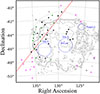 |
Fig. 1. Locations of all the 4FGL sources in the region of Vela, whose contours from a ROSAT observation are shown (Voges et al. 1999). The extended sources are labelled (blue circles), as well as the Vela pulsar. The squares represent the sources that we removed from the model (the sources in Table 1 except for those classified as pulsars) while the green triangles are the sources that were kept in the model (the sources classified as pulsars in Table 1 and those that might be associated with the Vela molecular ridge, i.e., the sources in Table 2). The sources that we kept in the model because they have known associations in the 4FGL catalogue or lie outside our chosen region around Vela (large dashed circle) are represented by magenta + symbols. The dashed red line represents the Galactic plane. |
2.3. Extension of the GeV emission
To improve the background model outside the selected region in Fig. 1, we applied the source-finding algorithm in fermipy that requires a TS > 16 and a separation of 0.2° from known sources, followed by a fit of the spectral normalisations of sources located within 10° of the ROI centre, the spectral parameters of the sources described in Section 2.1, and the normalisations of the diffuse components. We removed the 22 sources that were classified as nonAGN and nonPSR from the model (see Table 1). In order to model the residual emission we adopted a simple morphology given by a uniform disk, whose location and size were varied to maximise its TS. During this procedure, we kept the spectral parameters of all the sources located within 5° of the ROI centre free. We used a simple power-law spectral function for the disk, dN/dE = N0(E/E0)−Γ, with free normalisation and spectral index (N0 and Γ). E0 is a fixed scale that we set at the pivot energy, that is, the energy for which the propagated uncertainty in dN/dE is minimized. The resulting centre location and radius of the disk are (RA, Dec) =  ,
,  (the first error is statistical while the second systematic), and E0 = 2242 MeV. We estimated these systematic errors by repeating the analysis for each of the eight alternative models for the diffuse emission developed by Acero et al. (2016). In all these alternative models, we consistently found a larger emission region that is displaced to the south with respect to the disk found using the standard diffuse emission model, and thus we report asymmetric errors for Dec and r.
After adding the extended source and again fitting the spectral normalisations for all sources found within 10° of the ROI centre and the spectral indices of the sources located within 5°, we found a TS value for the disk of 2051.5, corresponding to a high detection significance of 45σ. The resulting spectral index is Γ ∼ 2.5. The emission from the pulsar was effectively suppressed, as the corresponding source, 4FGL J0835.3 − 4510, shows a TS of 84. For comparison, we performed an analysis without pulsar gating and obtained a value of the order of 106 for the TS of the pulsar.
In order to visualise the emission we removed the disk from the model and obtained a TS map by fitting the normalisation of a test point source at every pixel location assuming a simple power-law spectrum with an index of 2.5. The result is shown in Fig. 2. To assess the quality of the fit we also calculated a p-value statistic map (PS, a data-model deviation estimator) as defined by Bruel (2021). We optimised the map for residuals with a spatial scale of 1°, and it is shown in Fig. 2 in units of σ. Positive deviations are seen within the shell of the SNR in the southern and western portions, indicating that the uniform disk model adopted in this work is only an approximation of the morphology of the emission. We adopted this model for simplicity and left improvements for future work.
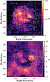 |
Fig. 2. Top: TS map of the Vela region in the energy range 1 − 100 GeV (note that the scale is not linear). Bottom: Residual PS map (see text). For both maps the contours are the same as in Fig. 1 and the large circle represents the disk found in this work. |
We calculated the Akaike information criterion (AIC, Akaike 1974) to compare the quality of the model with the extended source (AICext) and the original model with the 4FGL point sources (AICps). We fit the spectral parameters of the point sources and also considered the location, extension, and spectral parameters of the extended source as free in the respective models. The resulting difference is AICps−AICext = 192, indicating that the model with the extended source is highly preferred over the alternative using point sources.
2.4. Gamma-ray spectrum
We repeated the analysis in the entire energy range 0.1 − 100 GeV starting with the optimised model found in the previous section and again applied the source-finding algorithm to improve the background, as in Section 2.3. We fit the spectral normalisations of the sources found within 10° and all the spectral parameters of the sources within 5° of the RoI centre. When fitting a log-parabola for our disk of the form dN/dE = N0(E/E0)−α − β ln, (E/E0) (with N0, α, and β as free parameters and E0 = 1 GeV a fixed scale), the TS improves by ∼1400 with respect to the fit using a simple power law. The source spectrum is significantly curved and the resulting parameters are N0 = (7.76 ± 0.006 ± 4.0)×10−11 MeV−1 cm−2 s−1, α = 2.15 ± 0.0007 ± 0.04, and β = 0.23 ± 0.0004 ± 0.08 (the first error is statistical while the second is systematic). This can be seen in the spectral energy distribution ( ; SED; see plots below). We divided the data into 11 energy bins to estimate the flux values in each bin. For each energy bin, we fit the spectral parameters of the sources with TS > 100 and set the parameter cov_scale=5 to minimise overfitting and constrain the large number of free parameters with priors taken from the global fit. The resulting fluxes are shown in Table 3. We calculated flux upper limits at the 95% confidence level if the TS of the source is below four in a bin.
SED fluxes.
The source 4FGL J0843.9 − 4224c, which we classified as a pulsar candidate in Section 2.2, is not significantly detected with TS ∼ 6 and therefore we removed it from the model. Regarding the other sources that we classified as pulsar candidates, we obtained TS values of 568 (4FGL J0854.8 − 4504), 233 (4FGL J0853.6 − 4306), and 138 (4FGL J0900.1 − 4402c).
The integrated energy flux in the 1 − 100 GeV range is ∼1.9 × 10⁻¹⁰ erg cm−2 s−1, corresponding to a luminosity of 1.9 × 1033 erg s−1. For comparison, we estimate the GeV luminosity of Vela X as ∼1.4 × 1033 erg s−1 in the same energy range.
In order to calculate the systematic errors, we first considered uncertainties in the LAT’s effective area. We propagated the corresponding uncertainty in the spectral parameters by repeating the analysis using a set of bracketing response functions as in Ackermann et al. (2012). We also considered the effect of the choice of the eight alternative models for diffuse emission (Acero et al. 2016), as explained earlier. We repeated the analysis for each alternative diffuse emission model and obtained the corresponding SED fluxes. We added the uncertainties of the two effects described in quadrature, and the results are included in Table 3. Using the nominal Galactic diffuse emission model we did not detect the source in the last energy bin, 37.9 − 100 GeV. Using the alternative diffuse emission models, the source was not detected in the energy bin 14.4 − 37.9 GeV, or in the first bin, 0.1 − 0.17 GeV, for three out of the eight alternative models. We conservatively report upper limits for these three bins obtained with the likelihood profile using the nominal Galactic background model.
As noted by Acero et al. (2016), this approach yields a limited estimate of the systematic uncertainty rather than a complete determination. Even though there might be additional systematic effects due to the diffuse emission modelling that we did not account for, we believe that the significant detection of GeV photons across the shell of the SNR is strong evidence for its association with this object. We hereafter assume that the gamma rays are produced by Vela and we explore several models for their origin in the following section.
3. Discussion
3.1. SNR emission
It has been proposed that there is a uniform distribution of relativistic particles in the interior of the Vela SNR (Sushch & Hnatyk 2014). We used a one-zone model to fit the non-thermal emission from Vela with the naima package (Zabalza 2015) in two different scenarios. In the leptonic scenario the emission is caused by relativistic electrons. They interact with a magnetic field producing synchrotron emission, and inverse Compton (IC) scatter low energy photons to produce gamma rays. We took the synchrotron fluxes from the northern shell of the SNR (Vela Y, from Alvarez et al. 2001) as an approximation to the radio spectrum. We used the two photon fields from Tibaldo et al. (2018) to approximate the local interstellar radiation, given by greybody spectra with temperatures of 30 K (FIR) and 3000 K (NIR), and energy densities of 0.2 eV cm−3 and 0.3 eV cm−3, respectively, as well as the cosmic microwave background (CMB). The IC calculation is adopted from Khangulyan et al. (2014) and the synchrotron emissivity is taken from Aharonian et al. (2010). We also considered the average magnetic field as a free parameter. In the hadronic scenario, the gamma rays are produced in inelastic scatterings of cosmic ray protons off ambient protons. The parametrisation of the gamma-ray production cross-section from Kafexhiu et al. (2014) is implemented in the calculation.
To fit the SED fluxes, we used a differential particle distribution that follows a power law in momentum, p, of the form  , with s the spectral index. We also tested a power law with an exponential cutoff,
  , having an additional free parameter, pc. For the GeV data points we summed the statistical and systematic errors in quadrature to obtain the total error. We compared the fit results using the Bayesian information criterion (BIC) implemented within naima. The model with the lower BIC is favoured.
In the hadronic scenario, the power-law particle distribution gives an adequate fit (BIC = 5.9) and the cutoff is not required (BIC = 7.9). The data and the model are shown in Fig. 3. The spectral index is  and the total energy content in the hadrons is
  erg, where n is the average number density of the ambient material. This amount of energy could be provided by an SNR shock with a typical kinetic energy of the order of 1051 erg.
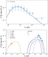 |
Fig. 3. Top: Gamma-ray fluxes and the hadronic model. The hadronic distribution used is a simple power law in momentum. Bottom: Leptonic model for the radio and gamma-ray emission from Vela for a particle momentum distribution, which is a power law with an exponential cutoff (the non-thermal X-ray flux measured by eROSITA is shown for comparison). |
In the leptonic scenario, it is not possible to simultaneously fit the radio and GeV fluxes with a simple power law for the particle distribution because it considerably over-predicts the GeV fluxes. Thus we used a power law with exponential cutoff. The resulting spectral index and cutoff momentum are  and
and  GeV/c (with c the speed of light), respectively. The magnetic field is
  μG and the total particle energy content is
  erg (integrated for particles with energies above 1 GeV). Since it is possible that the radio and GeV fluxes are produced by different leptonic populations, we performed fits to the GeV fluxes only, resulting in a BIC value of 15.1, which indicates that the hadronic model is highly preferred compared to the leptonic fit.
In the plot with the leptonic fit in Fig. 3 the approximate non-thermal flux of the X-ray nebula discovered by eROSITA (taken from Mayer et al. 2023, and thought to be produced by the pulsar) is shown for comparison in the 1 − 5 keV energy range. We estimated this non-thermal X-ray SED from their reported integrated flux assuming a spectrum that follows a simple power law with an index of three (Mayer et al. 2023). However, the spectral index of the nebula varies with location, and thus our estimate is only an approximation to the spectrum.
The estimated gamma-ray luminosity in the range 1 − 100 GeV of ∼3 × 1033 erg is relatively low compared to those of SNRs that interact with molecular clouds (Acero et al. 2016), but very similar to the luminosity of the Cygnus Loop (Katagiri et al. 2011) and of other relatively faint SNRs detected by the LAT (e.g. Araya 2013; Burger-Scheidlin et al. 2024; Araya 2024). As shown in Fig. 2, the GeV emission is prominent in the NE of the SNR. This is the region where the ambient density is higher and it could be interpreted as supporting the hadronic scenario. Dubner et al. (1998) showed evidence for the presence of an HI shell on the border of the Vela SNR, suggesting an association with the remnant. This emission seems more prominent in the N and NE of Vela; thus, the GeV emission seen in the NE outside the shell of the SNR could be produced by cosmic rays escaping from the object and reaching any atomic gas present. However, several star-forming regions are also seen in the direction outside the NE shell of the SNR located along the Vela molecular ridge, a cloud complex found further than the Vela SNR. More detailed work is needed to disentangle any contributions to the GeV emission from the SNR and these star-forming regions.
3.2. PWN emission
Mayer et al. (2023) recently discovered an X-ray synchrotron nebula that extends for several degrees beyond the known TeV emission region associated with the PWN. High-energy particles could have escaped Vela X in the past and produce GeV emission extending through the Vela SNR. From the point of view of the energetics, the total spin-down energy injected by the pulsar over its lifetime is more than sufficient to account for a particle content of ∼1048 erg (Abdo et al. 2010b), as required by the simple leptonic estimate in the previous section. The emission found in this work has a GeV spectrum that is softer than that reported for Vela X in the catalogue and comparable luminosity. First of all, the one-zone leptonic scenario presented in the previous section provides a relatively poor fit to the data. Furthermore, Hinton et al. (2011) have shown that the particles escaping from Vela X should produce GeV emission with a spectrum that is much harder and with considerably higher luminosity than what we found in the Vela SNR. Although our leptonic fit in the previous section is poor, it implies a particle cutoff energy of ∼300 GeV, while the highest energies of the escaping particles in their model are in the TeV range. Although a sufficiently high magnetic field could produce the spectral turnover, a magnetic field value of only a few μG is required to explain the extended X-ray nebula (Mayer et al. 2023). Detailed modelling is needed to explain the role, if any, that Vela’s pulsar could play in producing the GeV emission. However, the GeV emission found in this work cannot be produced by the same electrons responsible for the extended X-ray nebula. The typical energies of electrons that emit X-ray synchrotron emission in a magnetic field of a few μG are well into the TeV regime. A considerably extended TeV counterpart of the X-ray nebula will likely be revealed with future observations (for example by the SWGO experiment, SWGO Collaboration 2025).
4. Conclusions
GeV emission is seen across the shell of the Vela SNR after subtracting the contributions from the sources in the 4FGL LAT catalogue in the region. In addition to this emission, a cluster of unidentified point sources located mainly across the NE shell of the Vela SNR is found in the catalogue. This may indicate that the point sources are actually part of the SNR. We applied machine learning classification schemes to this set of sources and found that the majority do not share spectral features with those of known populations of GeV-emitting AGNs and pulsars, the most common types of point source in the LAT catalogues. We thus proposed that these point-like sources are part of the extended SNR. We modelled the emission with a simple geometrical template whose best-fit size is close to that of the Vela SNR, although it is displaced to the NE. The emission shows a high detection significance (∼45σ, 1 − 100 GeV). The GeV luminosity is similar to that of other SNRs. The spectrum of the gamma-ray emission and its spatial coincidence with regions of enhanced ambient density point to a hadronic origin, while a one-zone leptonic model provides the worst fit to the GeV fluxes. A contribution from the PWN Vela X is problematic due to the soft GeV spectrum of the observed emission, its relatively low luminosity compared to predictions from the population of leptons escaping from Vela X, and the difficulties in fitting the spectral shape with a leptonic model. More detailed models for the evolution of the system must be carried out in order to assess the role that Vela X could have played in producing the GeV photons. Future studies to characterise the gamma-ray emission on smaller angular scales throughout Vela are possible. In addition, the source classification scheme carried out in this work constitutes a curated analysis-ready corpus for Fermi-LAT sources in general, which may prove valuable for reproducibility of this work and for future independent studies of any sky region with the LAT.
Acknowledgments
We are grateful to the anonymous referee for providing a valuable review which helped improve this work. We also thank M. Kerr for the updated ephemeris of the Vela pulsar, and funding from Universidad de Costa Rica under grant number C4228.
References
- Abadi, M., Agarwal, A., Barham, P., et al. 2016, in 12th USENIX Symposium on Operating Systems Design and Implementation (OSDI 16), 265 [Google Scholar]
- Abdo, A. A., Ackermann, M., Ajello, M., et al. 2010a, ApJ, 713, 154 [NASA ADS] [CrossRef] [Google Scholar]
- Abdo, A. A., Ackermann, M., Ajello, M., et al. 2010b, ApJ, 713, 146 [NASA ADS] [CrossRef] [Google Scholar]
- Abdollahi, S., Acero, F., Ackermann, M., et al. 2020, ApJS, 247, 33 [Google Scholar]
- Abdollahi, S., Acero, F., Baldini, L., et al. 2022, ApJS, 260, 53 [NASA ADS] [CrossRef] [Google Scholar]
- Abdollahi, S., Acero, F., Acharyya, A., et al. 2024, arXiv e-prints [arXiv:2411.07162] [Google Scholar]
- Acero, F., Ackermann, M., Ajello, M., et al. 2016, ApJS, 224, 8 [NASA ADS] [CrossRef] [Google Scholar]
- Ackermann, M., Ajello, M., Albert, A., et al. 2012, ApJS, 203, 4 [Google Scholar]
- Aharonian, F., Akhperjanian, A. G., Bazer-Bachi, A. R., et al. 2006, A&A, 448, L43 [NASA ADS] [CrossRef] [EDP Sciences] [Google Scholar]
- Aharonian, F. A., Kelner, S. R., & Prosekin, A. Y. 2010, Phys. Rev. D, 82, 043002 [Google Scholar]
- Akaike, H. 1974, IEEE Trans. Autom. Control, 19, 716 [Google Scholar]
- Akiba, T., Sano, S., Yanase, T., Ohta, T., & Koyama, M. 2019, in Proceedings of the 25th ACM SIGKDD International Conference on Knowledge Discovery and Data Mining (ACM), 2623 [Google Scholar]
- Alvarez, H., Aparici, J., May, J., & Reich, P. 2001, A&A, 372, 636 [NASA ADS] [CrossRef] [EDP Sciences] [Google Scholar]
- Anderson, L. D., Bania, T. M., Balser, D. S., et al. 2014, ApJS, 212, 1 [Google Scholar]
- Araya, M. 2013, MNRAS, 434, 2202 [NASA ADS] [CrossRef] [Google Scholar]
- Araya, M. 2018, ApJ, 859, 69 [NASA ADS] [CrossRef] [Google Scholar]
- Araya, M. 2020, MNRAS, 492, 5980 [NASA ADS] [CrossRef] [Google Scholar]
- Araya, M. 2024, A&A, 691, A225 [NASA ADS] [CrossRef] [EDP Sciences] [Google Scholar]
- Araya, M., Gutiérrez, L., & Kerby, S. 2022, MNRAS, 510, 2277 [NASA ADS] [CrossRef] [Google Scholar]
- Aschenbach, B., Egger, R., & Trümper, J. 1995, Nature, 373, 587 [Google Scholar]
- Atwood, W. B., Abdo, A. A., Ackermann, M., et al. 2009, ApJ, 697, 1071 [CrossRef] [Google Scholar]
- Bhat, A., & Malyshev, D. 2022, A&A, 660, A87 [NASA ADS] [CrossRef] [EDP Sciences] [Google Scholar]
- Bocchino, F., Maggio, A., & Sciortino, S. 1999, A&A, 342, 839 [NASA ADS] [Google Scholar]
- Bruel, P. 2021, A&A, 656, A81 [NASA ADS] [CrossRef] [EDP Sciences] [Google Scholar]
- Burger-Scheidlin, C., Brose, R., Mackey, J., et al. 2024, A&A, 684, A150 [NASA ADS] [CrossRef] [EDP Sciences] [Google Scholar]
- Caraveo, P. A., De Luca, A., Mignani, R. P., & Bignami, G. F. 2001, ApJ, 561, 930 [Google Scholar]
- Chang, C.-C., & Lin, C.-J. 2011, ACM Trans. Intell. Syst. Technol., 2, 1 [CrossRef] [Google Scholar]
- Chiaro, G., Kovacevic, M., & La Mura, G. 2021, JHEAP, 29, 40 [Google Scholar]
- Cooper, N., Dainotti, M. G., Narendra, A., Liodakis, I., & Bogdan, M. 2023, MNRAS, 525, 1731 [Google Scholar]
- Cortes, C., & Vapnik, V. 1995, Mach. Learn., 20, 273 [Google Scholar]
- Cozzolongo, G., Mitchell, A. M. W., Spencer, S. T., Malyshev, D., & Unbehaun, T. 2025, in Proceedings of the 8th Heidelberg International Symposium on High-Energy Gamma-Ray Astronomy, [arXiv:2504.03543] [Google Scholar]
- Dodson, R., Legge, D., Reynolds, J. E., & McCulloch, P. M. 2003, ApJ, 596, 1137 [Google Scholar]
- Dubner, G. M., Green, A. J., Goss, W. M., Bock, D. C. J., & Giacani, E. 1998, AJ, 116, 813 [NASA ADS] [CrossRef] [Google Scholar]
- Fang, K., Bi, X.-J., & Yin, P.-F. 2019, MNRAS, 488, 4074 [NASA ADS] [CrossRef] [Google Scholar]
- Finke, T., Krämer, M., & Manconi, S. 2021, MNRAS, 507, 4061 [NASA ADS] [CrossRef] [Google Scholar]
- Frail, D. A., Bietenholz, M. F., & Markwardt, C. B. 1997, ApJ, 475, 224 [NASA ADS] [CrossRef] [Google Scholar]
- Ge, T.-T., Sun, X.-N., Yang, R.-Z., et al. 2024, MNRAS, 530, 1144 [Google Scholar]
- Géron, A. 2019, Hands-On Machine Learning with Scikit-Learn, Keras, and TensorFlow. Concepts, Tools, and Techniques to Build Intelligent Systems, 2nd edn. (O’Reilly Media, Inc.) [Google Scholar]
- Giuffrida, R., Lemoine-Gourmard, M., Miceli, M., et al. 2025, A&A, 701, A206 [NASA ADS] [CrossRef] [EDP Sciences] [Google Scholar]
- Grondin, M. H., Romani, R. W., Lemoine-Goumard, M., et al. 2013, ApJ, 774, 110 [Google Scholar]
- Hinton, J. A., Funk, S., Parsons, R. D., & Ohm, S. 2011, ApJ, 743, L7 [Google Scholar]
- Hobbs, G. B., Edwards, R. T., & Manchester, R. N. 2006, MNRAS, 369, 655 [Google Scholar]
- Huang, Z.-Q., Fang, K., Liu, R.-Y., & Wang, X.-Y. 2018, ApJ, 866, 143 [Google Scholar]
- Kafexhiu, E., Aharonian, F., Taylor, A. M., & Vila, G. S. 2014, Phys. Rev. D, 90, 123014 [Google Scholar]
- Katagiri, H., Tibaldo, L., Ballet, J., et al. 2011, ApJ, 741, 44 [NASA ADS] [CrossRef] [Google Scholar]
- Khangulyan, D., Aharonian, F. A., & Kelner, S. R. 2014, ApJ, 783, 100 [Google Scholar]
- Kohavi, R. 1995, in Proceedings of the 14th International Joint Conference on Artificial Intelligence (IJCAI) (Montreal, Quebec, Canada: Morgan Kaufmann), 1137 [Google Scholar]
- Kovacevic, M., Chiaro, G., Cutini, S., & Tosti, G. 2020, MNRAS, 493, 1926 [CrossRef] [Google Scholar]
- Lange, A., Eagle, J., Kargaltsev, O., Kuiper, L., & Hare, J. 2025, ApJ, 988, 200 [Google Scholar]
- Lu, F. J., & Aschenbach, B. 2000, A&A, 362, 1083 [NASA ADS] [Google Scholar]
- Malyshev, D. V., & Bhat, A. 2023, MNRAS, 521, 6195 [Google Scholar]
- Markwardt, C. B., & Ögelman, H. B. 1997, ApJ, 480, L13 [Google Scholar]
- Mattox, J. R., Bertsch, D. L., Chiang, J., et al. 1996, ApJ, 461, 396 [Google Scholar]
- Mayer, M. G. F., Becker, W., Predehl, P., & Sasaki, M. 2023, A&A, 676, A68 [NASA ADS] [CrossRef] [EDP Sciences] [Google Scholar]
- Pal, M., & Foody, G. M. 2010, IEEE Trans. Geosci. Remote Sens., 48, 2297 [Google Scholar]
- Pedregosa, F., Varoquaux, G., Gramfort, A., et al. 2011, J. Mach. Learn. Res., 12, 2825 [Google Scholar]
- Peron, G., Casanova, S., Gabici, S., Baghmanyan, V., & Aharonian, F. 2024, Nat. Astron., 8, 530 [CrossRef] [Google Scholar]
- Rangelov, B., Yang, H., Williams, B., et al. 2024, ApJ, 961, 26 [Google Scholar]
- Saz Parkinson, P. M., Xu, H., Yu, P. L. H., et al. 2016, ApJ, 820, 8 [NASA ADS] [CrossRef] [Google Scholar]
- Slane, P., Lovchinsky, I., Kolb, C., et al. 2018, ApJ, 865, 86 [Google Scholar]
- Sokolova, M., & Lapalme, G. 2009, Inform. Process. Manage., 45, 427 [Google Scholar]
- Sushch, I., & Hnatyk, B. 2014, A&A, 561, A139 [NASA ADS] [CrossRef] [EDP Sciences] [Google Scholar]
- Sushch, I., Hnatyk, B., & Neronov, A. 2011, A&A, 525, A154 [NASA ADS] [CrossRef] [EDP Sciences] [Google Scholar]
- SWGO Collaboration (Abreu, P., et al.) 2025, arXiv e-prints [arXiv:2506.01786] [Google Scholar]
- Ballet, J., Bruel, P., Burnett, T. H., & Lott, B., & The Fermi-LAT collaboration 2023, arXiv e-prints [arXiv:2307.12546] [Google Scholar]
- Tibaldo, L., Zanin, R., Faggioli, G., et al. 2018, A&A, 617, A78 [NASA ADS] [CrossRef] [EDP Sciences] [Google Scholar]
- Voges, W., Aschenbach, B., Boller, T., et al. 1999, A&A, 349, 389 [NASA ADS] [Google Scholar]
- Wood, M., Caputo, R., Charles, E., et al. 2017, in 35th International Cosmic Ray Conference (ICRC2017), 301, 824 [Google Scholar]
- Xiao, H., Cao, H., Fan, J., et al. 2020, Astron. Comput., 32, 100387 [Google Scholar]
- Zabalza, V. 2015, in 34th International Cosmic Ray Conference (ICRC2015), 34, 922 [Google Scholar]
- Zadrozny, B., & Elkan, C. in Proceedings of the Eighth ACM SIGKDD International Conference on Knowledge Discovery and Data Mining (KDD-2002) (Edmonton, Alberta, Canada: ACM), 694, 2002 [Google Scholar]
- Zhu, K. R., Chen, J. M., Zheng, Y. G., & Zhang, L. 2023, MNRAS, 527, 1794 [CrossRef] [Google Scholar]
Kindly provided to us by M. Kerr.
Architecture and training follow standard deep-learning practice for multi-class classification according to https://keras.io.
As implemented in scikit-learn (e.g. StratifiedShuffleSplit/StratifiedKFold).
All Tables
All Figures
|
Fig. 1. Locations of all the 4FGL sources in the region of Vela, whose contours from a ROSAT observation are shown (Voges et al. 1999). The extended sources are labelled (blue circles), as well as the Vela pulsar. The squares represent the sources that we removed from the model (the sources in Table 1 except for those classified as pulsars) while the green triangles are the sources that were kept in the model (the sources classified as pulsars in Table 1 and those that might be associated with the Vela molecular ridge, i.e., the sources in Table 2). The sources that we kept in the model because they have known associations in the 4FGL catalogue or lie outside our chosen region around Vela (large dashed circle) are represented by magenta + symbols. The dashed red line represents the Galactic plane. |
| In the text | |
|
Fig. 2. Top: TS map of the Vela region in the energy range 1 − 100 GeV (note that the scale is not linear). Bottom: Residual PS map (see text). For both maps the contours are the same as in Fig. 1 and the large circle represents the disk found in this work. |
| In the text | |
|
Fig. 3. Top: Gamma-ray fluxes and the hadronic model. The hadronic distribution used is a simple power law in momentum. Bottom: Leptonic model for the radio and gamma-ray emission from Vela for a particle momentum distribution, which is a power law with an exponential cutoff (the non-thermal X-ray flux measured by eROSITA is shown for comparison). |
| In the text | |
Current usage metrics show cumulative count of Article Views (full-text article views including HTML views, PDF and ePub downloads, according to the available data) and Abstracts Views on Vision4Press platform.
Data correspond to usage on the plateform after 2015. The current usage metrics is available 48-96 hours after online publication and is updated daily on week days.
Initial download of the metrics may take a while.