| Issue |
A&A
Volume 710, June 2026
|
|
|---|---|---|
| Article Number | A32 | |
| Number of page(s) | 9 | |
| Section | Galactic structure, stellar clusters and populations | |
| DOI | https://doi.org/10.1051/0004-6361/202557415 | |
| Published online | 28 May 2026 | |
3D kinematics of Small Magellanic Cloud star clusters: Residual velocities disentangle kinematically perturbed clusters
1
Instituto Interdisciplinario de Ciencias Básicas (ICB), CONICET-UNCuyo,
Padre J. Contreras 1300,
M5502JMA,
Mendoza,
Argentina
2
Consejo Nacional de Investigaciones Científicas y Técnicas (CONICET),
Godoy Cruz 2290,
C1425FQB,
Buenos Aires,
Argentina
★ Corresponding author: This email address is being protected from spambots. You need JavaScript enabled to view it.
Received:
25
September
2025
Accepted:
9
April
2026
Abstract
Understanding the kinematic behavior of the Small Magellanic Cloud (SMC) remains a challenge addressed by many authors using diverse approaches. Over time, increasing observational evidence has accumulated for tidal perturbations induced by the Large Magellanic Cloud (LMC) on the SMC, especially in its outer regions. In this study, we adopted star clusters as kinematic tracers of the SMC. We analyzed 36 clusters distributed across the galaxy's structural regions (Northern Bridge, Southern Bridge, Wing/Bridge, West Halo, Main Body and Counter Bridge). From each cluster's proper motions, radial velocity, and heliocentric distance, we estimated Cartesian velocities (Vx, Vy, Vz) in the SMC reference frame. We also computed the same velocity components under the assumption that the SMC behaves as a rotating disk. We then defined the residual velocity ΔV for each cluster as the difference between the two derived velocities. Additionally, we performed kinematic anisotropy analysis to characterize the distribution of kinetic energy across the SMC. We find that increasing values of ΔV correlate with increasing cluster distance from the SMC center, and that ΔV ≈ 60 km s−1 appears to be a kinematic lower limit separating the tidally originating areas from those with the best behavior.
Key words: galaxies: kinematics and dynamics / Magellanic Clouds / galaxies: star clusters: general
© The Authors 2026
 Open Access article, published by EDP Sciences, under the terms of the Creative Commons Attribution License (https://creativecommons.org/licenses/by/4.0), which permits unrestricted use, distribution, and reproduction in any medium, provided the original work is properly cited.
This article is published in open access under the Subscribe to Open model. This email address is being protected from spambots. You need JavaScript enabled to view it. to support open access publication.
1 Introduction
The kinematic behavior of the Small Magellanic Cloud (SMC) has been investigated in recent years by several authors (e.g., Kallivayalil et al. 2013; Zivick et al. 2018; De Leo et al. 2020; Niederhofer et al. 2021; Dhanush et al. 2025). Understanding the internal kinematics of the SMC is essential for reconstructing its interactions with the Large Magellanic Cloud (LMC) and the Milky Way.
To trace the kinematic signatures of the SMC, different galactic constituents have been used, including HI gas, young stars, red giant stars, massive stars, among others. Gas in the SMC exhibits considerable internal rotation (Stanimirović et al. 2004), while young stars show orderly motion toward the Magellanic Bridge, with proper motions exceeding those of the SMC Main Body (Oey et al. 2018). Indeed, Nakano et al. (2025) investigated the motions of massive stars (>8 M⊙) with ages <50 Myr; they found trajectories oriented toward the LMC and away from the SMC Main Body. In contrast, the oldest stellar population apparently shows little rotation (Harris & Zaritsky 2006; Zivick et al. 2021), making the SMC kinematics – in some respects – a persistent conundrum. We note, however, that some of these results are based solely on radial velocity (RV) or proper motion measurements.
The SMC is under tidal effects due to its interactions with the LMC (Mackey et al. 2018; Zivick et al. 2018; De Leo et al. 2020; Niederhofer et al. 2021; Omkumar et al. 2021). The magnitude and strength of tidal forces on the morphology and internal kinematics of the SMC were estimated from dynamic simulations by Besla et al. (2012). They concluded that the Magellanic Clouds are on their first infall toward the Milky Way. In this context, Piatti (2021a) used star clusters as tracers of the SMC's internal kinematics and constructed a 3D image of their motions from Gaia data (Gaia Collaboration 2016) and RV from the literature. The cluster motions derived by Piatti (2021a) show some notable dispersion around the resulting rotating disk. This finding reveals that SMC cluster kinematics is complex and cannot be fully captured by a representation of a rotating disk alone.
In this work, we analyzed 36 SMC star clusters with the aim of obtaining a comprehensive representation of the SMC's internal kinematics, based on heliocentric distances obtained by Illesca et al. (2025), proper motions retrieved from Gaia data release 3 (Gaia Collaboration 2016; Luri et al. 2021), and RVs available in the literature. Incorporating individual cluster heliocentric distances – rather than adopting a single SMC mean distance for all the clusters – makes the derived kinematic behaviors more robust. From this dataset, we constructed a 3D velocity map of the SMC, following the formalism of van der Marel et al. (2002). We then analyzed the residual velocities and explored the resulting kinematic signatures across known tidally perturbed SMC structures. In Sect. 2, we describe the data collected and employed in the present analysis. In Sect. 3, we describe our results, while in Sect. 4 we discuss the residual velocities of star clusters as indicators of kinematic perturbations caused by tidal forces. Section 5 summarizes the main conclusions of this work.
2 Data collection and processing
Illesca et al. (2025) studied 40 SMC star clusters, mainly distributed across the outer SMC regions, with the aim of investigating the connection between their ages, heliocentric distances, and metallicities. We used their cluster collection as a starting point to build a sample of SMC star clusters with the three fundamental parameters mentioned, in addition to RVs and proper motions. Unfortunately, as far as we know, 12 star clusters do not have RVs available in the literature (B88, B139, BS116, HW64, HW67, HW73, HW77, IC1655, L2, L3, L73, and L95). Therefore, we added eight other star clusters with the required information (L1, L8, L12, L68, L113, NGC 339, NGC 361, and NGC 419), taking their fundamental parameters taken from Piatti (2023). For the final sample of 36 star clusters (accurate individual cluster heliocentric distance was required), we extracted the clusters' right ascension (RA), declination (Dec), and radii from Bica et al. (2020). For the astrometric information, we retrieved from Gaia DR3 the proper motions in RA (pmra) and Dec (pmdec), parallaxes (ϖ), excess noise (epsi), significance of excess noise (sepsi), and G, BP, and RP magnitudes for every star located within three times the respective cluster radius. We applied a filter to the proper motion errors to retain those stars with σ ≤ 0.1 mas yr−1, following the procedure described in Piatti et al. (2019). We selected extragalactic stars by applying the condition |ϖ|/σ(ϖ) < 3. Furthermore, to improve our data quality, we limited sepsi<2, epsi<1, RUWE ≤ 1.4, and G ≤ 18 mag, respectively (see, e.g., Ripepi et al. 2019).
We then used the procedure devised by Piatti & Bica (2012), originally designed to clean star cluster color-magnitude diagrams from field star contamination, to statistically remove SMC field stars from the vector point diagrams (VPDs) of the star clusters. The statistical cleaning method uses comparison field regions surrounding each cluster. Figure 1 illustrates the locus of the cluster circle relative to eight circular comparison fields of the same area. The method superimposes the cluster and one comparison field VPD; for each star in the latter, it subtracts the closest star in the cluster VPD. Proper motion errors of the stars were also accounted for when searching for a star to subtract from the cluster VPD. To do this, we allowed the proper motions of the stars in the cluster VPD to vary within ±1σ. We repeated the procedure described above for one thousand comparison fields placed around the cluster's circle at randomly chosen position angles. Finally, we assigned cluster membership probabilities to the stars in the cluster VPD as P (%) = 100 × S /1000, where S represents the number of times the star was not subtracted over 1000 runs. An example is illustrated in Fig. 2. Stars with different P values were plotted with different colors. In our subsequent analysis, we retained only stars with P > 50%.
For the N stars in each cluster that satisfy the above restriction, we applied the effective sample size concept introduced by Kish (1987). We defined an effective N (Neff) as a representative, comparable measure of star-by-star kinematics. We computed Neff using the expression
 (1)
(1)
where
 (2)
(2)
In Eq. (2),  combines an individual star's membership probabilities pk, k = 1,…,N, with an average value
  . The first factor
  in Eq. (2) penalizes star clusters with low average membership probabilities, while the second factor
  penalizes clusters with fewer stars. This ratio corresponds to the effective sample size of Kish (1987). Here, Neff is the normalized version of
  , which we used in subsequent analysis as a relative quality weight for our star cluster kinematic results.
We applied a maximum likelihood statistical method (Meylan & Pryor 1993; Walker et al. 2006) to estimate the mean proper motions and dispersion of the studied clusters. In practice, we optimized the probability L to extract stars with proper motions (pmi) and errors σi from a population with mean proper motion 〈pm〉 and dispersion W, as follows:

where the mean and dispersion errors were calculated from respective covariance matrices. The resulting mean cluster proper motions are shown in Table A.1, alongside the number of stars (N) used to compute them.
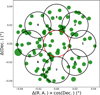 |
Fig. 1 Stars selected from Gaia DR3 distributed across NGC 416. The red circle marks the cluster field, while the black circles mark the eight different comparison fields adjacent to the cluster. The symbol sizes are proportional to stellar brightness in the G filter. |
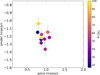 |
Fig. 2 VPD for the selected Gaia DR3 stars distributed across NGC 416. The color symbols vary according to assigned membership probability. |
3 Star cluster kinematic properties
We chose star clusters as kinematic tracers because they provide a robust methodology that distinguishes this approach from others. Unlike field star populations Dhanush et al. (2025), clusters are discrete, gravitationally bound objects. This enables more accurate estimates of their ages, distances, and velocities than for field stars. Moreover, our star cluster sample includes individual heliocentric distances – a valuable feature compared to kinematic models based on field stars, which employ mean distances and thus underestimate the role of distance.
As kinematic tracers, stellar clusters provide an insightful view into SMC kinematics without the biases that other tracers might introduce due to the lack of distance estimates. Although Dhanush et al. (2025) performed a differential analysis by population to account for changes in geometry and, consequently, in the kinematic model, we used the SMC kinematic model obtained by Piatti (2021a), which is based on star clusters. He found that the SMC rotation disk is characterized by a center at RA = 13.30° ± 10, Dec = −72.85° ± 10; a distance to center 59 ± 1.5 kpc, RV (150 ± 2 km s−1); central proper motions pmracenter = 0.75 ± 10 mas yr−1, pmdeccenter = −1.26 ± 0.05 mas yr−1 ; disk inclination 70° ± 10; line of nodes (LONs) position angle 200 ± 30; and rotation velocity 25 ± 5.0 km s−1.
We first subtracted the mean proper motion and RV of the SMC center of mass (Piatti 2021a) from the resulting clusters' mean proper motions and RVs to calculate the residual linear velocities VRV, VRA, and VDec, (the latter in kilometers per second) using the expression 4.7403885 × D [mas yr−1], where D is the cluster heliocentric distance.To convert the vector (VRV, VRA, VDec) into one with components Vx and Vy in the plane of the SMC and Vz perpendicular to it, we used the reference system defined by van der Marel et al. (2002) and followed the procedure described in Piatti et al. (2019). This comprised inverting the matrix A = B × C, where B is the matrix

with b1, b2, b3, and b4 being the coefficients of transformation from Eq. (9), and C is the matrix defined in Eq. (5) of van der Marel et al. (2002), so that
 (3)
(3)
The errors σ(Vx), σ(Vy), and σ(Vz) were estimated via Monte Carlo experiments using the uncertainties in VRV, VRA and VDec and VDec. From Eq. (3) we calculated  and
and  . The resulting values are listed in Table A.2.
In addition, we computed the velocity components (Vx′, Vy′, Vz′) with respect to the SMC center that the star clusters would have if they rotated at their present positions in the SMC disk according to the rotation disk fitted by Piatti (2021a). The difference between (Vx, Vy, Vz) and (Vx, Vy, Vz') gives the so-called residual velocity vector (ΔVx, ΔVy, ΔVz), where ΔVx = Vx – Vx', ΔVy = Vy – Vy', and ΔVz = Vz – Vz'. The resulting values are listed in Table A.3. The module of the residual velocity vector  was introduced by Piatti (2021b) as a measure of the kinematic perturbation experienced by a star cluster, i.e., how much the cluster's motion departs from ordered rotation.
Finally, following van der Marel & Cioni (2001), we computed the Cartesian coordinates (x, y, z) of the star clusters with respect to the SMC center:
![Mathematical equation: $\matrix{ {x = D\sin \rho \cos \left( {\phi - \theta } \right),} \hfill \cr {y = D\left[ {\sin \rho \cos i\sin \left( {\phi - \theta } \right) + \cos \rho \sin i} \right] - {D_0}\sin i,} \hfill \cr {z = D\left[ {\sin \rho \cos i\sin \left( {\phi - \theta } \right) - \cos \rho \sin i} \right] - {D_0}\cos i,} \hfill \cr }$](/articles/aa/full_html/2026/06/aa57415-25/aa57415-25-eq14.png) (4)
(4)
where D, ρ, and ϕ are the cluster heliocentric distances, the cluster projected distances from the SMC center, and their position angles, respectively computed from the cluster celestial coordinates (RA, Dec). The value DO represents the mean heliocentric distance of the SMC center (62.44 kpc, Graczyk et al. 2020), while θ and i represent the position angle of the LONs and the inclination of the SMC disk derived by Piatti (2021a). From Eq. (4), we computed the projected distance on the SMC plane  and the 3D distance
  . We list the resulting values in Table A.3. At first glance, most selected star clusters are distributed within R3D ~ 14 kpc, with a few reaching R3D ~ 25 kpc (see Figure 3).
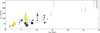 |
Fig. 3 Rotational velocity values for the studied star clusters as a function of their distances to the SMC center. The colors represent different structures of the SMC (Dias et al. 2016), as indicated in the top-right panel (NB=Northern Bridge, MB=Main Body, SB=Southern Bridge, W/B=Wing/Bridge, and WH=West Halo). The symbol sizes are proportional to Neff. |
4 Analysis and discussion
Besla et al. (2012) showed that the irregular morphology and internal kinematics of the Magellanic System can be more robustly explained by considering gravitational interactions between the LMC and the SMC. This outcome leads to questions about the kinematic signatures witnessing the tidally disturbed structures of the SMC. We here addressed this issue by using star clusters as kinematic tracers and their residual velocities as a measure of the perturbed kinematic signatures. In this context, star clusters located in tidally perturbed SMC regions are expected to have larger residual velocities. For instance, Piatti (2021a, see his Fig. 3) found that star clusters in the outer SMC regions (some with known tidal origin) have ΔV > 50 km s−1 . We built a similar figure (see Fig. 5), using our sample of 36 star clusters. As shown, star clusters outside the SMC Main Body have ΔV > 60 km s−1, while smaller ΔV values are mostly seen for star clusters in the SMC Main Body. Moreover, the closer star clusters are to the Sun, the larger their residual velocities, which could be a direct measure of the tidal interaction strength with the LMC (mean heliocentric distance ~49.9 kpc; de Grijs et al. 2014).
Figure 6 shows the sky distribution of the studied star clusters with the outer SMC regions separated by dashed lines: Northern Bridge (NB), Wing/Bridge (W/B), Southern Bridge (SB), West Halo (WH), and Counter Bridge (CB) (Dias et al. 2016). Star clusters are colored according to their dispersion velocities, with those having larger ΔV values mainly distributed in the outer SMC regions. These regions are known to have been affected by LMC tides (e.g., Zivick et al. 2018; Schmidt et al. 2020; Dias et al. 2022; Parisi et al. 2024; Mackey et al. 2018); thus, the derived larger ΔV values could measure the strength of LMC tidal effects. For instance, L116, located in the Southern Bridge region, has a residual velocity of 225.73 km s−1 and is moving toward the LMC. In the West Halo, L4, 11, and 13 exhibit residual velocities greater than 110 km s−1, with velocity vectors oriented toward the opposite direction of the LMC.
Both the Wing/Bridge and the Northern Bridge also have star clusters with relatively high residual velocities pointing toward the LMC (see Table A.2). Star clusters located in the SMC Main Body or surrounding it generally have residual velocities of ΔV < 60 km s−1. A 3D space view of the residual velocities is depicted in Fig. 4. As can be seen, the SMC is more elongated along the x-axis (approximately parallel to the SMC line of sight), with increasing residual velocities from its center out to its outskirts.
To characterize the kinematics of clusters in different substructures with possible tidal origin, we analyzed the dispersion of their 3D residual velocity components and compared them to the total dispersion. Following the work of Watkins et al. (2024), we introduced kinematic anisotropy in the SMC framework as follows:
 (5)
(5)
for i = x, y, z.
Figure 7 shows the values of Ax, Ay, and Az as a function of galactocentric distance for each of the SMC disk models proposed in Piatti (2026). At first glance, star clusters in the outer regions of the SMC show greater anisotropy along the x- and z-axes, suggesting overall agitated kinematics approximately parallel to the SMC line of sight and perpendicular to its plane.
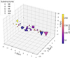 |
Fig. 4 3D distribution of our studied star clusters. Star clusters projected onto different SMC substructures are represented by different symbols, with colors corresponding to their residual velocities. The symbol sizes are proportional to Neff. |
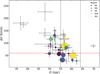 |
Fig. 5 Residual velocities as a function of the heliocentric distances of the studied star clusters. The vertical dashed lines represent the boundaries of the SMC Main Body (Piatti 2021a), while the horizontal red line represents the lower residual velocity limit adopted in this work for the star clusters outside the SMC Main Body. Star clusters pertaining to different substructures (Dias et al. 2016) are drawn in different colors, as indicated in the top-right panel. The symbol sizes are proportional to Neff. |
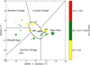 |
Fig. 6 Sky distribution of the studied star clusters, colored according to their residual velocities. The dashed lines delimit the different outer SMC regions (Illesca et al. 2025). The symbols sizes are proportional to Neff. |
4.1 West Halo
The West Halo was proposed by Dias et al. (2016) as a substructure distant from the Main Body of the SMC and confirmed by proper motion studies (Niederhofer et al. 2018; Piatti 2021a). Moreover, Tatton et al. (2020) suggested that the West Halo could be the tidal counterpart of the SMC Bridge (see also Zivick et al. 2018).
We obtain Ax = 0.72, Ay = 0.17, and Az = 0.11, with a spatial depth of ~ 17 kpc in star cluster distribution, indicating clear elongation and predominant motion dispersion along the x-axis (see Fig. 4).These outcomes reinforce the hypothesis that the West Halo is a dispersed, disturbed substructure, possibly originating from detachment of the SMC Main Body (Dias et al. 2022).
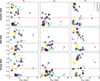 |
Fig. 7 Distribution of Ax, Ay, and Az as a function of distance from the SMC center (R3D). Anisotropy was estimated for each of the models studied in Piatti (2026). Top: cluster disk model (Piatti 2021a). Middle: old disk model (age >2 Gyr). Bottom: young disk model (age < 50 Myr). Star clusters pertaining to different substructures (Dias et al. 2016) are drawn in different colors, as indicated in the top-right panel. The red line (Ai = 0.33, i = x, y, z) represents the expected value for an isotropic motion. The symbol sizes are proportional to Neff. |
4.2 Bridges and wing
For the Wing/Bridge region, we obtain Ax = 0.68, Ay = 0.09, and Az = 0.23. This result suggests that the star clusters are moving toward the LMC, as is also the case for the star clusters in the Southern Bridge (Ax = 0.51, Ay = 0.06, and Az = 0.44). Four of the six star clusters analyzed in this region have residual velocities higher than the threshold value listed in Fig. 5 (62 km s−1) and heliocentric distances smaller than 55 kpc, which could indicate escaping motions. On the other hand, star clusters in the Northern Bridge show predominant motion dispersion perpendicular to the SMC plane (Ax = 0.16, Ay = 0.29, and Az = 0.55). Three are located close to the boundary of the SMC Main Body, while the other four are placed at heliocentric distances shorter than 51 kpc. Once again, the correlation between the residual velocity amplitude and the heliocentric distance reinforces their tidal origin (Piatti 2022; Sakowska et al. 2024).
4.3 Main Body
The studied star clusters projected onto the SMC Main Body span ~ 23.5 kpc in heliocentric distance, with B99 and H86-97 being the closest to the Sun (D < 39 kpc). These two star clusters have ΔV > 170 km s−1, which distinguishes them from those physically occupying the SMC Main Body (ΔV < 60 km s−1).
4.4 Kinematics under different SMC disk models
As previously noted by Piatti (2026), estimating ΔV depends on the adopted SMC rotation disk. Therefore, a comprehensive analysis of the kinematics of the studied star clusters requires considering different rotation disk models. Dhanush et al. (2025) used Gaia DR3 data to derive kinematic parameters for different SMC star populations. From young to old star populations, they found a change in the SMC disk inclination from ~82° to ~58°, and in the position angle of the LONs from ~180° to ~240°. Following the three SMC rotation disk models analyzed in Piatti (2026) (see Table A.4), we computed, for each kinematic scenario, the corresponding AV and the anisotropy along each SMC axis using a Monte Carlo approach. The relations between anisotropy and each cluster's distance from the SMC center for the three disk models are shown in Fig. 5.
From the estimated global anisotropy, we obtain for the old disk model Ax = 0.61, Ay = 0.15, and Az = 0.23. For the Piatti (2021a) model, we find Ax = 0.63, Ay = 0.13, and Az = 0.24. Finally, for the young disk model, we obtain Ax = 0.72, Ay = 0.04, and Az = 0.24.
These values indicate more dispersed, dynamically perturbed kinematics along the line of sight (the x-axis) in the young disk scenario. In contrast, the old disk and Piatti (2021a) models show lower dispersion, although dominant agitation still occurs along the galaxy's line of sight. Our results for the young disk scenario are fully consistent with the findings of Piatti (2026) and Dhanush et al. (2025), in which star clusters exhibit a gradient in kinematic agitation as their distances from the SMC center increase. Nevertheless, analyzing the results for the Piatti (2021a) and old disk models reveals no well-behaved kinematic distribution along the three axes of the galaxy, contrary to expectations for our cluster sample with a mean age of ~3 Gyr.
In this context, it is important to examine several key aspects. First, the clusters selected for this study are mostly located in external SMC substructures. Thus, although the aforementioned models may capture the average agitation of older clusters, clusters in regions such as the West Halo or the Southern Bridge introduce a level of perturbation so high that their velocities exceed any average rotational behavior. For instance, the cluster L116 in the Southern Bridge exhibits a ΔV of 225.73 km s−1, moving toward the LMC. This parameter likely places it outside any disk orbit, even a perturbed one.
Another important aspect is that, although the Piatti (2021a) and old disk models adopt different geometries compared to the young-cluster model, their geometries are still inferred from present-day observations. In other words, they do not fully represent the original disk geometry at the epoch of cluster formation or LMC tidal force interaction. Furthermore, we used individual heliocentric distances in the equations to derive each cluster's velocities. This provides additional robustness to the determination of ΔV and the corresponding anisotropy.
It is therefore likely that the parameters of the Piatti (2021a) and old disk models do not accurately reflect the magnitude of the kinematic agitation affecting old clusters in the outer regions of the SMC. Our work does not aim to settle this debate, but rather to highlight the complexity involved in addressing SMC kinematics.
5 Conclusions
The SMC is currently understood to be gravitationally bound to the LMC. Their interactions have left imprints on the SMC's formation and evolution. Star clusters are fundamental building blocks of any galaxy, so it is reasonable to expect that they may contain valuable information about the SMC's dynamical history.
In this work, we analyzed 36 star clusters in the SMC to derive their 3D velocities and explore the relationship between star cluster kinematics and tidal forces, particularly in the SMC's outer regions. We used proper motions from Gaia DR3, RVs taken from the literature, and our derived heliocentric distances. From these data, we derived 3D velocities and their residual velocities. Our main findings can be summarized as follows:
The lower threshold for the residual velocities of the star clusters in outer SMC regions is ΔV ≈ 60 km s−1. This result is in very good agreement with the value derived by Piatti (2021b). Star clusters belonging to the SMC Main Body mostly show lower ΔV values, thus confirming more tightly disk-like kinematics;
We performed an anisotropy analysis for different SMC disk models (Piatti 2026), based on recent findings by Dhanush et al. (2025) linking the kinematics of the SMC with the age of the analyzed stellar sample. Although we find kinematic differences for each disk model, we also find certain regularities in relation to the kinematics and external substructures of the SMC: the West Halo, the Wing/Bridge, the northern and the Southern Bridges show greater kinematic dispersion along the x-axis (approximately parallel to the SMC line of sight) and perpendicular to the disk, while star clusters in the SMC Main Body retain some amount of coherent rotation;
Our heliocentric distances (Piatti 2023; Illesca et al. 2025) allowed us to construct a more realistic internal reference frame for the SMC. We thus report a line-of-sight depth of ~25 kpc for the studied star cluster sample;
Building a 3D map of the SMC from the derived positions of each star cluster, combined with their residual velocities and substructure membership, enabled us to identify spatial-velocity dispersion correlations;
Our subregion-by-subregion analysis reveals an overall kinematic picture of the SMC with kinematically hot outer regions, a pattern consistent with tidal models and recent close-encounter scenarios between both Magellanic Clouds (Rathore et al. 2024).
Acknowledgements
We thank the referee for the thorough reading of the manuscript and timely suggestions to improve it. This work has made use of data from the European Space Agency (ESA) mission Gaia (https://www.cosmos.esa.int/gaia), processed by the Gaia Data Processing and Analysis Consortium (DPAC, https://www.cosmos.esa.int/web/gaia/dpac/consortium). Data for reproducing the figures and analyses in this work will be available upon request to the first author.
References
- Besla, G., Kallivayalil, N., Hernquist, L., et al. 2012, MNRAS, 421, 2109 [Google Scholar]
- Bica, E., Westera, P., Kerber, L. d. O., et al. 2020, VizieR Online Data Catalog: J [Google Scholar]
- De Bortoli, B. J., Parisi, M. C., Bassino, L. P., et al. 2022, A&A, 664, A168 [NASA ADS] [CrossRef] [EDP Sciences] [Google Scholar]
- de Grijs, R., Wicker, J. E., & Bono, G. 2014, AJ, 148, 17 [NASA ADS] [CrossRef] [Google Scholar]
- De Leo, M., Carrera, R., Noël, N. E., et al. 2020, MNRAS, 495, 98 [Google Scholar]
- Dhanush, S., Subramaniam, A., & Subramanian, S. 2025, ApJ, 980, 73 [Google Scholar]
- Dias, B., Kerber, L., Barbuy, B., Bica, E., & Ortolani, S. 2016, A&A, 591, A11 [NASA ADS] [CrossRef] [EDP Sciences] [Google Scholar]
- Dias, B., Angelo, M. S., Oliveira, R. A. P. d., et al. 2021, A&A, 647, L9 [NASA ADS] [CrossRef] [EDP Sciences] [Google Scholar]
- Dias, B., Parisi, M. C., Angelo, M., et al. 2022, MNRAS, 512, 4334 [NASA ADS] [CrossRef] [Google Scholar]
- Gaia Collaboration, (Prusti, T., et al.) 2016, A&A, 595, A1 [NASA ADS] [CrossRef] [EDP Sciences] [Google Scholar]
- Graczyk, D., Pietrzynski, G., Thompson, I. B., et al. 2020, ApJ, 904, 13 [Google Scholar]
- Harris, J., & Zaritsky, D. 2006, ApJ, 131, 2514 [Google Scholar]
- Illesca, D. M., Piatti, A. E., Chiarpotti, M., & Butrón, R. 2025, A&A, 696, A244 [NASA ADS] [CrossRef] [EDP Sciences] [Google Scholar]
- Kallivayalil, N., Van der Marel, R. P., Besla, G., Anderson, J., & Alcock, C. 2013, ApJ, 764, 161 [NASA ADS] [CrossRef] [Google Scholar]
- Kish, L. 1987, Surv. Statist., 17, 26 [Google Scholar]
- Luri, X., Chemin, L., Clementini, G., et al. 2021, A&A, 649, A7 [NASA ADS] [CrossRef] [EDP Sciences] [Google Scholar]
- Mackey, D., Koposov, S., Da Costa, G., et al. 2018, ApJ, 858, L21 [Google Scholar]
- Meylan, G., & Pryor, C. 1993, Struct. Dyn. Glob. Clusters, 50, 31 [Google Scholar]
- Nakano, S., Tachihara, K., & Tamashiro, M. 2025, ApJS, 277, 62 [Google Scholar]
- Niederhofer, F., Cioni, M.-R., Rubele, S., et al. 2018, A&A, 613, L8 [NASA ADS] [CrossRef] [EDP Sciences] [Google Scholar]
- Niederhofer, F., Cioni, M.-R. L., Rubele, S., et al. 2021, MNRAS, 502, 2859 [Google Scholar]
- Oey, M., Jones, J. D., Castro, N., et al. 2018, ApJ, 867, L8 [NASA ADS] [CrossRef] [Google Scholar]
- Omkumar, A. O., Subramanian, S., Niederhofer, F., et al. 2021, MNRAS, 500, 2757 [Google Scholar]
- Parisi, M., Grocholski, A., Geisler, D., Sarajedini, A., & Clariá, J. 2009, ApJ, 138, 517 [Google Scholar]
- Parisi, M. C., Geisler, D., Clariá, J. J., et al. 2015, ApJ, 149, 154 [Google Scholar]
- Parisi, M. C., Gramajo, L. V., Geisler, D., et al. 2022, A&A, 662, A75 [NASA ADS] [CrossRef] [EDP Sciences] [Google Scholar]
- Parisi, M., Oliveira, R., Angelo, M., et al. 2024, MNRAS, 527, 10632 [Google Scholar]
- Piatti, A. E. 2021a, A&A, 650, A52 [NASA ADS] [CrossRef] [EDP Sciences] [Google Scholar]
- Piatti, A. E. 2021b, MNRAS, 508, 3748 [Google Scholar]
- Piatti, A. E. 2022, MNRAS, 509, 3462 [Google Scholar]
- Piatti, A. E. 2023, MNRAS, 526, 391 [Google Scholar]
- Piatti, A. E. 2026, A&A, 706, A343 [NASA ADS] [CrossRef] [EDP Sciences] [Google Scholar]
- Piatti, A. E., & Bica, E. 2012, MNRAS, 425, 3085 [Google Scholar]
- Piatti, A. E., Alfaro, E. J., & Cantat-Gaudin, T. 2019, MNRAS, 484, L19 [Google Scholar]
- Rathore, H., Choi, Y., Olsen, K. A., & Besla, G. 2024, ApJ, 978, 55 [Google Scholar]
- Ripepi, V., Molinaro, R., Musella, I., et al. 2019, A&A, 625, A14 [NASA ADS] [CrossRef] [EDP Sciences] [Google Scholar]
- Sakowska, J. D., Noël, N. E. D., Ruiz-Lara, T., et al. 2024, MNRAS, 532, 4272 [Google Scholar]
- Schmidt, T., Cioni, M.-R. L., Niederhofer, F., et al. 2020, A&A, 641, A134 [NASA ADS] [CrossRef] [EDP Sciences] [Google Scholar]
- Song, Y.-Y., Mateo, M., Bailey J. I., III, et al. 2021, MNRAS, 504, 4160 [NASA ADS] [CrossRef] [Google Scholar]
- Stanimirović, S., Staveley-Smith, L., & Jones, P. 2004, ApJ, 604, 176 [Google Scholar]
- Tatton, B., Van Loon, J. T., Cioni, M. L., et al. 2020, MNRAS, 504, 2983 [Google Scholar]
- van der Marel, R. P., & Cioni, M.-R. L. 2001, ApJ, 122, 1807 [Google Scholar]
- van der Marel, R. P., Alves, D. R., Hardy, E., & Suntzeff, N. B. 2002, ApJ, 124, 2639 [Google Scholar]
- Walker, M. G., Mateo, M., Olszewski, E. W., et al. 2006, ApJ, 131, 2114 [Google Scholar]
- Watkins, L. L., van der Marel, R. P., & Bennet, P. 2024, ApJ, 963, 84 [NASA ADS] [CrossRef] [Google Scholar]
- Zivick, P., Kallivayalil, N., van der Marel, R. P., et al. 2018, ApJ, 864, 55 [Google Scholar]
- Zivick, P., Kallivayalil, N., & van der Marel, R. P. 2021, ApJ, 910, 36 [Google Scholar]
Appendix A Collected and derived kinematic parameters of star clusters
Proper motions and RVs of the studied star clusters.
Space velocity components of the star clusters.
Residual velocity components of star cluster.
SMC rotation disk models.
All Tables
All Figures
|
Fig. 1 Stars selected from Gaia DR3 distributed across NGC 416. The red circle marks the cluster field, while the black circles mark the eight different comparison fields adjacent to the cluster. The symbol sizes are proportional to stellar brightness in the G filter. |
| In the text | |
|
Fig. 2 VPD for the selected Gaia DR3 stars distributed across NGC 416. The color symbols vary according to assigned membership probability. |
| In the text | |
|
Fig. 3 Rotational velocity values for the studied star clusters as a function of their distances to the SMC center. The colors represent different structures of the SMC (Dias et al. 2016), as indicated in the top-right panel (NB=Northern Bridge, MB=Main Body, SB=Southern Bridge, W/B=Wing/Bridge, and WH=West Halo). The symbol sizes are proportional to Neff. |
| In the text | |
|
Fig. 4 3D distribution of our studied star clusters. Star clusters projected onto different SMC substructures are represented by different symbols, with colors corresponding to their residual velocities. The symbol sizes are proportional to Neff. |
| In the text | |
|
Fig. 5 Residual velocities as a function of the heliocentric distances of the studied star clusters. The vertical dashed lines represent the boundaries of the SMC Main Body (Piatti 2021a), while the horizontal red line represents the lower residual velocity limit adopted in this work for the star clusters outside the SMC Main Body. Star clusters pertaining to different substructures (Dias et al. 2016) are drawn in different colors, as indicated in the top-right panel. The symbol sizes are proportional to Neff. |
| In the text | |
|
Fig. 6 Sky distribution of the studied star clusters, colored according to their residual velocities. The dashed lines delimit the different outer SMC regions (Illesca et al. 2025). The symbols sizes are proportional to Neff. |
| In the text | |
|
Fig. 7 Distribution of Ax, Ay, and Az as a function of distance from the SMC center (R3D). Anisotropy was estimated for each of the models studied in Piatti (2026). Top: cluster disk model (Piatti 2021a). Middle: old disk model (age >2 Gyr). Bottom: young disk model (age < 50 Myr). Star clusters pertaining to different substructures (Dias et al. 2016) are drawn in different colors, as indicated in the top-right panel. The red line (Ai = 0.33, i = x, y, z) represents the expected value for an isotropic motion. The symbol sizes are proportional to Neff. |
| In the text | |
Current usage metrics show cumulative count of Article Views (full-text article views including HTML views, PDF and ePub downloads, according to the available data) and Abstracts Views on Vision4Press platform.
Data correspond to usage on the plateform after 2015. The current usage metrics is available 48-96 hours after online publication and is updated daily on week days.
Initial download of the metrics may take a while.