| Issue |
A&A
Volume 710, June 2026
|
|
|---|---|---|
| Article Number | A91 | |
| Number of page(s) | 9 | |
| Section | Catalogs and data | |
| DOI | https://doi.org/10.1051/0004-6361/202558722 | |
| Published online | 02 June 2026 | |
ARCAFF: Cutout classification dataset
1
Department of Mathematics, University of Genova,
via Dodecaneso 35,
16146
Genova,
Italy
2
Astronomy & Astrophysics Section, School of Cosmic Physics, Dublin Institute for Advanced Studies,
31 Fitzwilliam Place,
Dublin 2,
D02 XF86,
Ireland
3
Istituto Nazionale di Astrofisica, Osservatorio Astrofisico di Torino,
via Osservatorio 20,
10025
Pino Torinese,
Italy
★ Corresponding author: This email address is being protected from spambots. You need JavaScript enabled to view it.
Received:
22
December
2025
Accepted:
16
April
2026
Abstract
Context. Solar active regions (ARs) are dynamic and magnetically complex areas on the Sun’s surface, often associated with phenomena such as solar flares and coronal mass ejections. Accurate identification and classification of these regions are essential for understanding solar magnetic activity and forecasting space weather events. Traditional AR classification methods have predominantly relied on manual observation and analysis, which, while effective, are time-consuming and subject to human bias. Existing datasets for AR classification have significant limitations that hinder their effectiveness for deep-learning applications.
Aims. We present ARCAFF:CCD (Active Region Classification and Flare Forecasting: Cutout Classification Dataset), a new large-scale dataset of solar AR magnetograms and continuum cutouts specifically designed for machine-learning applications.
Methods. The dataset combines co-temporal line-of-sight magnetograms and continuum intensity images from the SOHO/MDI and SDO/HMI instruments. Each cutout is linked to AR identifiers assigned by the National Oceanic and Atmospheric Administration (NOAA) and includes both Mount Wilson and McIntosh classifications. The pipeline performs calibration, alignment, and structured labelling of full-disc magnetograms using AR classification metadata from NOAA Solar Region Summary (SRS) reports.
Results. The dataset covers nearly three decades of observations spanning multiple solar cycles, comprising 33 045 AR cutouts and 72 297 quiet Sun cutouts. Each cutout is accompanied by comprehensive metadata and, to our knowledge, represents the most extensive and detailed publicly available resource of its kind.
Conclusions. The ARCAFF:CCD dataset provides a comprehensive resource for developing and testing machine-learning models for solar AR classification and space weather forecasting.
Key words: methods: data analysis / techniques: image processing / catalogs / Sun: magnetic fields
© The Authors 2026
 Open Access article, published by EDP Sciences, under the terms of the Creative Commons Attribution License (https://creativecommons.org/licenses/by/4.0), which permits unrestricted use, distribution, and reproduction in any medium, provided the original work is properly cited.
This article is published in open access under the Subscribe to Open model. This email address is being protected from spambots. You need JavaScript enabled to view it. to support open access publication.
1 Introduction
Solar active regions (ARs) are dynamic and magnetically complex areas on the Sun’s surface, often associated with phenomena such as solar flares and coronal mass ejections (Tandberg-Hanssen & Emslie 1988; Piana et al. 2022; Webb & Howard 2012; Howard et al. 2023). Accurate identification and classification of these regions are essential for understanding solar magnetic activity and forecasting space weather events that can impact Earth’s technological infrastructures (Guastavino et al. 2022, 2023; Georgoulis et al. 2024; Pandey et al. 2022; Pilipenko 2021; Temmer 2021).
Traditional AR classification methods have predominantly relied on manual observation and analysis, which, while effective, are time-consuming and subject to human bias. Over the past three decades, space-based telescopes such as the Michelson Doppler Imager on board the Solar and Heliospheric Observatory (SOHO/MDI) (Scherrer et al. 1991) and the Helioseismic and Magnetic Imager on board the Solar Dynamics Observatory (SDO/HMI) (Scherrer et al. 2012) have produced an extensive collection of full-disc magnetograms and continuum images. This wealth of information makes AR classification an ideal target for automated, data-driven approaches based on modern machine-learning and deep-learning techniques (Fang et al. 2019; Tang et al. 2021; Legnaro et al. 2025).
However, existing datasets for AR classification have significant limitations that hinder their effectiveness for supervised-learning applications. For example, the SOLAR-STORM 1 dataset (Fang et al. 2019) does not provide explicit AR identifiers, such as National Oceanic and Atmospheric Administration (NOAA) numbers, or an AR-level data structure. As a result, repeated observations cannot be grouped and analysed by AR, which limits both the construction of training, validation, and test partitions at the AR level and the study of model behaviour on a per-region basis.
Similarly, while specialised automated extraction products such as the Spaceweather HMI Active Region Patch (SHARP) and the Spaceweather MDI Active Region Patch (SMARP) provide detailed vector and line-of-sight magnetogram data, they do not include explicit AR classification labels (e.g. Mount Wilson or McIntosh classes). Using these products for supervised learning therefore requires gathering and merging external classification information from independent sources. Additionally, SHARP and SMARP cutouts have variable spatial sizes, reflecting the automatically detected patch boundaries, and are produced through different processing pipelines for the two instruments. These characteristics make it more difficult to assemble a homogeneous cross-instrument dataset with consistent region definitions and preprocessing.
In response to these limitations, the present paper introduces ARCAFF:CCD (Active Region Classification and Flare Forecasting: Cutout Classification Dataset), a large-scale dataset of solar AR cutouts specifically designed for machine-learning applications. The ARCAFF:CCD dataset combines co-temporal line-of-sight magnetograms and continuum intensity images from SOHO/MDI and SDO/HMI, spans multiple solar cycles, and links each cutout to NOAA AR identifiers, as well as Mount Wilson and McIntosh classifications. To our knowledge, this is the most extensive publicly available dataset of its kind specifically tailored to supervised learning on ARs.
This paper is organised as follows. Section 2 details the data sources and procedures used to build the ARCAFF:CCD dataset, including the acquisition and processing of NOAA Solar Region Summary (SRS) classifications, magnetogram and continuum observations, and the generation of AR cutouts. Section 3 presents the classification schemes adopted, along with the distribution of Mount Wilson and McIntosh classes across the dataset. In particular, Section 3.3 describes the quality flag statistics and summarises the per-cutout magnetic and photometric properties, highlighting the dataset’s coverage and diversity. Section 4 presents a compact case study in magnetic classification and outlines other immediate learning tasks enabled by the dataset. Finally, we provide our concluding remarks in Section 5, together with notes on the public release of ARCAFF:CCD.
2 Dataset construction and data sources
The pipeline used to build the ARCAFF:CCD dataset performs calibration, alignment, and structured labelling of full-disc magnetograms using AR classification metadata. This section outlines the main components of the process, which consists of integrating SOHO/MDI and SDO/HMI full-disc magnetograms and continuum full-disc images with NOAA SRS reports to generate temporally aligned and consistently labelled AR cutouts. The main Python libraries used to build this dataset are NumPy (Harris et al. 2020), Astropy (Robitaille et al. 2013), SunPy (The SunPy Community et al. 2020)1 and Pandas (The pandas development team 2020)2. The end-to-end codebase used to construct the dataset is open source and available online3. Figure 1 shows a flowchart of the whole pipeline.
2.1 NOAA SRS classifications
We obtained AR classification metadata from the SRS reports issued by the NOAA Space Weather Prediction Center (SWPC) (Crown 2012). We retrieved the SRS data using SunPy’s unified search and retrieval tool, Fido, and subsequently parsed them with the read_srs method (SunPy Community et al. 2020). To allow the inclusion of earlier data, the read_srs method was updated as part of this work to accommodate SRS files produced before the year 2000. These legacy files differ structurally from modern formats, featuring uppercase section headers and supplementary tables following the standard sections (I, IA, and II), which previously caused parsing errors. The updated implementation introduces case-insensitive header detection and logic to correctly interpret these appended sections, allowing for complete ingestion of historical SRS records into the unified dataset. We developed this enhancement in coordination with the SunPy community and integrated it into the official library via GitHub Issue #70344 and Pull Request #70355. Related improvements include fixes to the Data Record Management System (DRMS) client submitted as a pull request sunpy/drms#1026, which address issues reported in sunpy/drms#987.
Figure 2 (left panel) presents the results of the SRS data processing in the form of a coverage plot. Some SRS reports were missing, and a small number of reports could not be parsed. Each SRS report can contain multiple ARs, and individual ARs may appear in consecutive daily reports for up to 13 days due to solar rotation. Each unique NOAA number represents a distinct classification instance; the same active region may reappear after rotating off the visible solar disc and returning after 14 days, but it will be assigned a new NOAA number.
We used the SRS reports to construct time series for individual ARs. Figure 2 (right panel) illustrates four of these time series, depicting the paths traced by ARs across the solar disc. Ideally, ARs follow the solar sidereal rotation rate of approximately 14 degrees per day in longitude, with minimal variation in latitude (around 0 degrees per day). To ensure consistency, we filtered the rate of change in both longitude and latitude to within ±7.5 degrees per day of the expected values. This filtering process identified and removed 1337 erroneous positions associated with 1261 ARs, resulting in a final dataset of 35 101 classifications across 5213 unique ARs. We detail the spatial distributions of the ARs in Section 3.
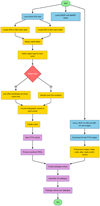 |
Fig. 1 End-to-end workflow used to construct the ARCAFF:CCD dataset. The diagram summarises all major processing steps, from ingesting NOAA SRS reports and instrument metadata to generating heliographic coordinates, extracting AR and quiet Sun cutouts, producing FITS and quicklook images, and assembling the final catalogue and packaged dataset. |
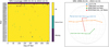 |
Fig. 2 Left: SRS coverage from 1 January 1995, 00:00 UT, to 30 December 2022, 00:00 UT. Right: traces of the progression of several ARs across the solar disc. The traces for NOAA ARs 7946, 8090, and 8238 show examples of issues in the reported data and have been removed from the dataset. |
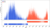 |
Fig. 3 Number of AR cutouts retained per day in the final sample for MDI (blue) and HMI (red) from 1996 to 2022. Top panel: daily AR counts for each instrument; bottom panel: dates on which observations are available for the two instruments. |
2.2 Magnetograms and continuum data
To complement the NOAA SRS data, we acquired daily line-ofsight magnetograms from 1996 to 2022, sampled at 00:00 UT each day to align with the validity time of NOAA SRS reports (issued at 00:30 UT). The last included observation date is 30 December 2022. We chose the 2022 cutoff to reserve more recent data for operational-style testing. By excluding the most recent observations, we retain a temporally forward dataset that can be used to evaluate models in a setting that more closely resembles real-world deployment, where models are applied to future, unseen active regions. We obtained the observations from SOHO/MDI and SDO/HMI from the Joint Science Operations Center (JSOC) at Stanford University. In addition to magnetograms, we retrieved the corresponding photospheric continuum intensity images for the same dates. Figure 3 shows the temporal distribution of the retained AR sample together with the observation coverage of the two instruments. Between 2010 and 2011, there are co-temporal observations of the line-of-sight magnetic field. For HMI magnetograms, we used the 12-minute cadence hmi.M_720s series. We used the continuum data series hmi.Ic_noLimbDark_720s, which corresponds to the SDO/HMI 720-second continuum intensity data with limb darkening removed. In the data-generation pipeline, we first associated SRS-filtered active-region records with the target day, and then we queried and downloaded the closest available hmi.M_720s full-disc magnetogram to 00:00 UT. We corrected the line-of-sight component by dividing by μ (the cosine of the heliocentric angle), under the standard assumption of a purely radial magnetic field, i.e. Bradial ≈ BLOS/μ. This μ-correction is a standard approximation, but it can be inaccurate in active regions, where strongly non-radial field components may distort structures such as polarity inversion lines. Because the dataset stores one full-disc snapshot per day at this reference time, these products are point-in-time observations and not synoptic maps (which are constructed over a full solar rotation).
The SOHO/MDI and SDO/HMI instruments have different resolutions and noise properties and are located in distinct positions and at varying distances from the Sun. Consequently, we processed the data to compensate for these discrepancies. We applied a preliminary data processing routine to full-disc MDI and HMI images to rotate them to solar north and remove off-disc data.
The SHARP (Bobra et al. 2014) and SMARP (Bobra et al. 2021) series are specialised data sets that automatically identify and extract ARs from full-disc solar images. These AR patches are analogous to NOAA AR numbers, but include additional detailed information from both vector and line-of-sight magnetogram data.
In addition to magnetograms and continuum intensity images, SHARP and SMARP patches provide data products such as Doppler velocity maps, error maps, and bitmaps marking active pixels. Each patch is assigned a unique HMI Active Region Patch (HARP) identifier for HMI or MDI Tracked Active Region Patch (TARP) identifier for MDI, which is mapped to NOAA AR numbers using external catalogues maintained by JSOC at Stanford University. This mapping process enables the association of SHARP and SMARP regions with NOAA classifications, facilitating pixel-level classification and the generation of bounding boxes for AR detection tasks.
We then generated bitmap segments from the full-disc images. These segments assign a value to each pixel based on its location (for example, whether it is on or off the solar disc or within an AR) and its line-of-sight magnetic field strength (strong or weak). This pixel-level encoding makes it possible to quickly isolate regions of interest, such as AR patches, from the vast amount of data contained in the full-disc images.
2.3 AR cutouts
Using the NOAA SRS classifications described in Section 2, we extracted AR locations and labels from the daily SRS files. We then used these locations, combined with a predefined region size, to crop magnetograms and continuum cutouts from the full-disc images. The cutouts have a 2:1 aspect ratio. For MDI they are 200 × 100 pixels, while for HMI they are 800 × 400 pixels. We did not resample the MDI data to the HMI sampling grid; instead, we kept both instruments at their native spatial resolution, which is why HMI cutouts contain four times more pixels in each dimension. We chose the cutout size to cover the full AR around the NOAA coordinates while keeping a consistent aspect ratio and sufficient spatial context for machine-learning inputs. In addition to ‘I’ regions, we retained ‘IA’ (H-alpha plage regions without sunspots), and we generated random quiet Sun (QS) regions – patches of non-active photosphere – to serve as negative examples in tasks that distinguish ARs from non-active regions. We sampled QS cutouts on each full-disc observation from non-overlapping locations that do not contain NOAA active regions or plage, using the same fixed-size windows as the AR cutouts (200 × 100 pixels for MDI and 800 × 400 pixels for HMI) and the same geometric preprocessing pipeline.
In addition to the magnetogram and continuum cutouts, we associated each region with SHARP- and SMARP-derived products (e.g., Doppler velocity maps, error maps, and active-pixel bitmaps; see Section 2.2). We mapped each patch identifier to the corresponding NOAA AR number using JSOC catalogues maintained at Stanford University, ensuring reliable linkage between cutouts and classification metadata.
The resulting AR classification dataset comprises 33 045 AR cutouts and 72 297 QS cutouts. The QS count is therefore not arbitrary but corresponds to the total number of valid QS samples obtained across all dates after applying these spatial exclusion constraints. Each cutout retains its associated McIntosh and Mount Wilson classification labels from the SRS reports.
2.4 Catalogue structure and metadata
Each cutout in ARCAFF:CCD is accompanied by a comprehensive set of metadata describing its heliographic coordinates, associated NOAA identifiers and classifications, file paths, instrument-specific quality flags, and geometric information used for alignment and extraction. This information is distributed with a tabular catalogue in which each row corresponds to a single cutout and the columns store both physical properties and processing-level attributes.
Table 1 lists all columns included in the released catalogue. We provide instrument-dependent fields separately for HMI and MDI; missing values for instruments that are not applicable to a given row are encoded as -.
3 Dataset characterisation
The ARCAFF:CCD dataset is accompanied by comprehensive metadata and quality indicators that describe the physical, morphological, and instrumental properties of each AR cutout. In particular, every cutout is linked to its NOAA identifier and includes both Mount Wilson and McIntosh classifications, along with instrument-specific quality flags and per-image statistical summaries. This section outlines these classification schemes and the overall statistical properties of the dataset.
Figure 4 illustrates the spatial and heliographic distribution of the AR cutouts included in the ARCAFF:CCD dataset. The left panel displays a density map of all extracted cutouts in heliographic coordinates and reveals the typical clustering of active regions along the solar activity belts at latitudes between ±15° and ±20°. This distribution shows the known butterfly pattern of sunspot emergence throughout the solar cycle (Hathaway 2015). The longitudinal histogram (centre) indicates a nearly uniform coverage across the solar disc, although a clear asymmetry is visible, with fewer ARs detected near the eastern limb than near the western limb. This imbalance arises from two main factors: (i) the intrinsic difficulty of identifying ARs near the solar limb, where projection effects reduce feature visibility; and (ii) the fact that AR positions are reported at different times during the day and are later differentially rotated to 00:00 UTC, occasionally displacing regions beyond the visible hemisphere. The latitudinal histogram (right) highlights the hemispheric symmetry of solar activity and the dominance of low-latitude active regions, consistent with the large-scale organisation of the solar dynamo.
3.1 Mount Wilson classification
The Mount Wilson classification scheme categorises solar active regions based on their magnetic field complexity as observed in magnetograms. The main classes are: α (unipolar), β (bipolar), β–γ (complex bipolar), β–δ (bipolar with strong opposite polarity umbrae within one penumbra), β–γ–δ (complex with strong opposite polarity umbrae), γ (complex, irregular), γ–δ, and FB (follower–bipolar). This scheme is widely used for space weather forecasting and research.
In addition to the Mount Wilson classes, the SRS reports include other region types:
IA: H-alpha plage regions without sunspots, indicating magnetic activity but lacking visible spots.
II: regions expected to return, i.e. those that have rotated off the visible disc and are anticipated to reappear.
For deep-learning applications, QS regions are generated by randomly sampling non-overlapping boxes that do not contain ARs or plage, serving as reference or background examples. Figure 5 (top panel) shows the distribution of these classes.
Columns in the ARCAFF:CCD region classification catalogue.
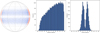 |
Fig. 4 Spatial and heliographic distributions of AR cutouts in the ARCAFF:CCD dataset. Left: heliographic map showing the locations of all extracted AR cutouts. Cutouts with longitude greater than ±65° are highlighted in red (the quantisation of the positions arises from latitude and longitude being stored as integers in the SRS reports). Centre and right: histograms of the corresponding longitude and latitude distributions, respectively. Longitudes show the expected bias against detections near the limbs, while the latitude distribution reflects the activity belts of solar cycles. |
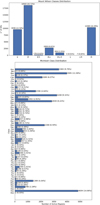 |
Fig. 5 Distribution of AR classes in the ARCAFF:CCD dataset. Top: Mount Wilson (magnetic) class distribution. Bottom: McIntosh class distribution. |
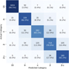 |
Fig. 6 Confusion matrix for a deit_base_patch16_224 model on the five-class QS, IA, α, β, and β–γ classification task using magnetogram cutouts from ARCAFF:CCD. The dominant errors occur between neighbouring magnetic-complexity levels, particularly α versus β and β versus β–γ. |
3.2 McIntosh classification
The McIntosh classification scheme provides a more detailed morphological description of sunspot groups than the Mount Wilson scheme, capturing their structure, penumbral development, and evolutionary stage. Each McIntosh class is composed of three components: the Zurich class (overall group type), the penumbral class (extent and development of penumbrae), and the compactness class (distribution of spots within the group). This system enables a nuanced characterisation of ARs, supporting studies of sunspot evolution and flare prediction. We include the McIntosh classification for each AR cutout in ARCAFF:CCD, as extracted from the NOAA SRS reports.
Figure 5 shows the distributions of the Mount Wilson and McIntosh classes in the ARCAFF:CCD dataset.
3.3 Quality flag distribution
We assigned each observation in the dataset a QUALITY flag, stored as a 32-bit integer, which encodes instrument and processing conditions at the time of acquisition. We used separate flag sets for SOHO/MDI and SDO/HMI data, following the definitions in the respective instrument documentation. We include the exact hexadecimal QUALITY value for each cutout in the released catalogue; here we summarise only the dominant states, since the remaining composite combinations are individually rare.
For SOHO/MDI, 42754 cutouts (58.67%) have QUALITY=0x00000000, while 28 692 (39.37%) correspond to the shutterless-mode state 0x00000200. All remaining MDI flag combinations occur in less than 0.6% of the sample.
For SDO/HMI, 65961 cutouts (99.20%) have QUALITY=0x00000000. The most common non-zero states are 0x00001000 (partial or missing frame; 173 cutouts, 0.26%) and 0x00000400 (shutterless mode; 148 cutouts, 0.22%); all remaining HMI flag combinations occur in less than 0.11% of the sample.
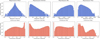 |
Fig. 7 Summary statistics for magnetogram (top row) and continuum (bottom row) data in ARCAFF:CCD. For each cutout, we show the mean, standard deviation, minimum, and maximum pixel values. Magnetogram values are line-of-sight magnetic field strengths in gauss. Continuum values are dimensionless normalised intensity. |
3.4 Cutout statistics
For the ARs present in the dataset, each cutout in ARCAFF:CCD is stored with per-image summary statistics for both the line-ofsight magnetic field (magnetogram) and the continuum intensity. For each cutout, we record, among other quantities, the pixel-wise mean, standard deviation, minimum, and maximum, along with the number of valid (non-NaN) pixels and the fraction of missing pixels.
Figure 7 shows the distributions of these quantities across all N = 33 045 AR cutouts. For the magnetograms (top row), the distribution of per-cutout mean field is narrowly centred around zero, reflecting the typical balance of opposite polarities in ARs. The per-cutout standard deviation of the magnetic field peaks around ~70 G and spans more than an order of magnitude, indicating that ARCAFF:CCD includes both weak, simple regions and magnetically complex, flare-productive regions. Individual pixels in the strongest regions reach instantaneous line-of-sight field strengths of the order ±5 kG. For continuum (bottom row), most cutouts have a mean normalised intensity close to unity, as expected for photospheric quiet background with sunspots, while the standard deviation is generally low but shows a high-variance tail due to deep sunspot umbrae and strong penumbrae. The continuum minima cluster near 0, corresponding to dark sunspot cores, and the continuum maxima extend above unity due to bright plage and facular enhancements.
3.5 Limitations and known issues
This section highlights some inherent limitations that arise from the underlying data sources and extraction procedure. First, since every cutout is extracted using a uniform spatial extent around the reported heliographic position, the resulting patch may include more than one NOAA region or fragments of nearby activity. This is particularly common during phases of dense activity or when NOAA numbers are assigned to substructures that lie very close together. Consequently, a cutout labelled with a single NOAA identifier can include additional regions that are not part of the intended target.
Moreover, the classification labels of Hale and McIntosh schemes originate from daily SRS reports, which are manually compiled. These labels can contain inconsistencies, occasional transcription errors, and day-to-day variability in expert assignment. Even after filtering for outliers in the SRS time series, some residual noise is unavoidable. For machine-learning workflows, this manifests primarily as imperfect supervision: two visually similar cutouts may have different assigned labels, while visually distinct regions may occasionally share the same label due to human subjectivity or reporting delays.
We illustrate these limitations in Figure 8, which shows sample data from the dataset. The full-disc views show several NOAA regions located in close proximity, and the corresponding cutouts on the right reveal overlap between multiple targets. In addition, the example containing AR 11987 illustrates that the μ-correction can introduce an incorrect polarity inversion line in some AR configurations.
Through exploratory data analysis (EDA) we find that some SoHO/MDI observations are marked as good quality according to the instrument quality flags but nevertheless display substantial data degradation. Figure 9 presents examples of such corrupted MDI full-disc magnetograms. The GitHub repository provides a list of the affected dates so that users can filter them out if necessary.
4 Case study: Magnetic classification
The released cutouts and metadata support Hale and Mount Wilson classification from magnetograms, continuum images, or their combination, as well as McIntosh classification and full-disc active-region localisation and classification. After flare-event labels are associated with the catalogue, they can also be used for point-in-time flare forecasting. We will present these applications in detail in a dedicated paper. For completeness, we include a compact case study based on a simple, reproducible baseline experiment to illustrate a supervised-learning setting.
We considered a five-class classification task on individual cutouts, distinguishing QS, IA, α, β, and β–γ. We excluded the rare γ and γ–δ classes, while β–δ is merged with β and β–γ–δ with β–γ, since the δ label acts as an additional qualifier on top of the underlying β or β–γ configuration rather than defining a fully separate large-scale morphology. We obtained training, validation, and test subsets with grouped stratification on the NOAA AR number, so that observations of the same AR do not leak across splits while the class distribution is approximately preserved. Magnetograms are HardTanh-normalised to [–1, 1] with d = 800, and we applied data augmentation on the fly through flips, perspective transforms, and affine perturbations. We used the resulting images to train image-classification models from the timm library (Wightman 2019). In the example shown below, we use the deit_base_patch16_224 architecture, trained with weighted cross-entropy, the Adam optimiser, mixed precision, and early stopping.
Figure 6 shows the resulting confusion matrix on the held-out test set. We recover the QS and IA classes well (96.5% and 82.5% recall, respectively), while the main ambiguities occur between neighbouring magnetic-complexity classes: α regions are most often confused with β, and β–γ regions with β.
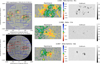 |
Fig. 8 Examples of HMI cutouts from the ARCAFF:CCD dataset. Left: full-disc magnetograms and continuum images with NOAA bounding boxes overlaid. Right: corresponding extracted cutouts. Some regions overlap (AR 11986 with AR 11987; AR 11982 with AR 11981; and IA 11983 and IA 11984). |
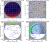 |
Fig. 9 Examples of corrupted MDI magnetograms present in the dataset, despite being flagged as good quality. Quality flags for these full discs are 0x00000000 (good quality) for April 20, 1999 and 0x00000200 (shutterless mode) for the remaining three. |
5 Conclusions
In this study, we introduced and analysed a novel dataset of solar magnetogram and continuum cutouts for ARs, the ARCAFF:CCD dataset, spanning observations from SOHO/MDI and SDO/HMI over two full solar cycles. The dataset is accompanied by detailed metadata (e.g. NOAA AR numbers and classifications), making it, to our knowledge, the most extensive and freely available dataset tailored for deep-learning applications of its kind. The following key points summarise the main contributions.
By covering multiple solar cycles and including both MDI and HMI observations, the dataset captures a broad range of AR manifestations and evolutionary stages. Its size, scope, and associated metadata address prior limitations of existing solar datasets, enabling more robust and AI-based approaches.
To illustrate this practical use, Section 4 presents a compact case study of magnetic classification, showing that the released cutouts and labels already support non-trivial supervised-learning benchmarks.
More broadly, ARCAFF:CCD enables several deep-learning applications. The released magnetogram and continuum cutouts support Hale or Mount Wilson classification from magnetograms, continuum images, or their combination; the accompanying metadata enable McIntosh classification; and the full-disc products and associated region information can be used for active-region localisation and classification. In addition, once flare-event labels are associated with the catalogue through NOAA active-region numbers and observation times, the same data can support point-in-time flare forecasting studies.
Although ARCAFF:CCD was designed primarily for machine-learning applications, it can also support a range of non-deep-learning studies in solar physics. The standardised HMI and MDI cutouts, together with the accompanying metadata, make it suitable for long-term statistical analyses of AR properties across solar cycles, comparative studies between instruments, and benchmarking of conventional image-processing or feature-detection pipelines, for example for sunspot identification, polarity-inversion-line extraction, or the detection of other magnetic structures.
In future work, we plan to describe the full-disc component of the dataset in more detail and to present a dedicated deep-learning paper that reports broader benchmarks on the cutoutand full-disc-based tasks enabled by ARCAFF:CCD.
Although the dataset has inherent limitations (such as potential spatial overlap of nearby regions, label inconsistencies in manual SRS classifications, and data quality issues in some MDI observations), these are thoroughly documented in Section 3.5 to enable users to make informed decisions about data filtering and preprocessing.
By making the dataset and our methods publicly available, we hope to facilitate ongoing collaborative progress in AI–driven solar physics research.
Data availability
The ARCAFF:CCD dataset is publicly available on Zenodo at https://doi.org/10.5281/zenodo.17865447.
Acknowledgements
All authors acknowledge the HORIZON Europe ARCAFF Project, Grant No. 101082164. E.L., S.G., M.P., A.M.M. acknowledge INdAMGNCS. M.P. acknowledges the support of the PRIN PNRR 2022 Project “Inverse Problems in the Imaging Sciences (IPIS)”, cup: D53D23005740006. This research was supported in part by the MIUR Excellence Department Project awarded to Dipartimento di Matematica, Università di Genova, CUP D33C23001110001.
References
- Bobra, M. G., Sun, X., Hoeksema, J. T., et al. 2014, Sol. Phys., 289, 3549 [Google Scholar]
- Bobra, M. G., Wright, P. J., Sun, X., & Turmon, M. J. 2021, ApJS, 256, 26 [Google Scholar]
- Crown, M. D. 2012, Space Weather, 10 [Google Scholar]
- Fang, Y., Cui, Y., & Ao, X. 2019, Adv. Astron., 2019, 9196234 [Google Scholar]
- Georgoulis, M. K., Yardley, S. L., Guerra, J. A., et al. 2024, Adv. Space Res., https://doi.org/10.1016/j.asr.2024.02.030 [Google Scholar]
- Guastavino, S., Marchetti, F., Benvenuto, F., Campi, C., & Piana, M. 2022, A&A, 662, A105 [NASA ADS] [CrossRef] [EDP Sciences] [Google Scholar]
- Guastavino, S., Marchetti, F., Benvenuto, F., Campi, C., & Piana, M. 2023, Front. Astron. Space Sci., 9, 1039805 [CrossRef] [Google Scholar]
- Harris, C. R., Millman, K. J., Van Der Walt, S. J., et al. 2020, Nature, 585, 357 [NASA ADS] [CrossRef] [Google Scholar]
- Hathaway, D. H. 2015, Living Rev. Sol. Phys., 12, 4 [Google Scholar]
- Howard, R. A., Vourlidas, A., & Stenborg, G. 2023, Front. Astron. Space Sci., 10, 1264226 [NASA ADS] [CrossRef] [Google Scholar]
- Legnaro, E., Guastavino, S., Piana, M., & Massone, A. M. 2025, ApJ, 981, 157 [Google Scholar]
- The pandas development team 2020, https://doi.org/10.5281/zenodo.3509134 [Google Scholar]
- Pandey, C., Ji, A., Angryk, R. A., Georgoulis, M. K., & Aydin, B. 2022, Front. Astron. Space Sci., 9, 897301 [NASA ADS] [CrossRef] [Google Scholar]
- Piana, M., Emslie, A. G., Massone, A. M., & Dennis, B. R. 2022, Hard X-Ray Imaging of Solar Flares, 164 (Springer) [Google Scholar]
- Pilipenko, V. 2021, Sol.-Terr. Phys., 7, 68 [Google Scholar]
- Robitaille, T. P., Tollerud, E. J., Greenfield, P., et al. 2013, A&A, 558, A33 [NASA ADS] [CrossRef] [EDP Sciences] [Google Scholar]
- Scherrer, P., Hoeksema, J., & Bush, R. 1991, Adv. Space Res., 11, 113 [Google Scholar]
- Scherrer, P. H., Schou, J., Bush, R., et al. 2012, Sol. Phys., 275, 207 [Google Scholar]
- SunPy Community, Barnes, W. T., Bobra, M. G., et al. 2020, ApJ, 890, 68 [NASA ADS] [CrossRef] [Google Scholar]
- Tandberg-Hanssen, E., & Emslie, A. G. 1988, The Physics of Solar Flares (Cambridge) [Google Scholar]
- Tang, R., Zeng, X., Chen, Z., et al. 2021, ApJS, 257, 38 [Google Scholar]
- Temmer, M. 2021, Living Rev. Sol. Phys., 18, 4 [Google Scholar]
- The SunPy Community, Barnes, W. T., Bobra, M. G., et al. 2020, ApJ, 890, 68 [NASA ADS] [CrossRef] [Google Scholar]
- Webb, D. F., & Howard, T. A. 2012, Living Rev. Sol. Phys., 9, 3 [Google Scholar]
- Wightman, R. 2019, PyTorch Image Models, https://github.com/rwightman/pytorch-image-models [Google Scholar]
All Tables
All Figures
|
Fig. 1 End-to-end workflow used to construct the ARCAFF:CCD dataset. The diagram summarises all major processing steps, from ingesting NOAA SRS reports and instrument metadata to generating heliographic coordinates, extracting AR and quiet Sun cutouts, producing FITS and quicklook images, and assembling the final catalogue and packaged dataset. |
| In the text | |
|
Fig. 2 Left: SRS coverage from 1 January 1995, 00:00 UT, to 30 December 2022, 00:00 UT. Right: traces of the progression of several ARs across the solar disc. The traces for NOAA ARs 7946, 8090, and 8238 show examples of issues in the reported data and have been removed from the dataset. |
| In the text | |
|
Fig. 3 Number of AR cutouts retained per day in the final sample for MDI (blue) and HMI (red) from 1996 to 2022. Top panel: daily AR counts for each instrument; bottom panel: dates on which observations are available for the two instruments. |
| In the text | |
|
Fig. 4 Spatial and heliographic distributions of AR cutouts in the ARCAFF:CCD dataset. Left: heliographic map showing the locations of all extracted AR cutouts. Cutouts with longitude greater than ±65° are highlighted in red (the quantisation of the positions arises from latitude and longitude being stored as integers in the SRS reports). Centre and right: histograms of the corresponding longitude and latitude distributions, respectively. Longitudes show the expected bias against detections near the limbs, while the latitude distribution reflects the activity belts of solar cycles. |
| In the text | |
|
Fig. 5 Distribution of AR classes in the ARCAFF:CCD dataset. Top: Mount Wilson (magnetic) class distribution. Bottom: McIntosh class distribution. |
| In the text | |
|
Fig. 6 Confusion matrix for a deit_base_patch16_224 model on the five-class QS, IA, α, β, and β–γ classification task using magnetogram cutouts from ARCAFF:CCD. The dominant errors occur between neighbouring magnetic-complexity levels, particularly α versus β and β versus β–γ. |
| In the text | |
|
Fig. 7 Summary statistics for magnetogram (top row) and continuum (bottom row) data in ARCAFF:CCD. For each cutout, we show the mean, standard deviation, minimum, and maximum pixel values. Magnetogram values are line-of-sight magnetic field strengths in gauss. Continuum values are dimensionless normalised intensity. |
| In the text | |
|
Fig. 8 Examples of HMI cutouts from the ARCAFF:CCD dataset. Left: full-disc magnetograms and continuum images with NOAA bounding boxes overlaid. Right: corresponding extracted cutouts. Some regions overlap (AR 11986 with AR 11987; AR 11982 with AR 11981; and IA 11983 and IA 11984). |
| In the text | |
|
Fig. 9 Examples of corrupted MDI magnetograms present in the dataset, despite being flagged as good quality. Quality flags for these full discs are 0x00000000 (good quality) for April 20, 1999 and 0x00000200 (shutterless mode) for the remaining three. |
| In the text | |
Current usage metrics show cumulative count of Article Views (full-text article views including HTML views, PDF and ePub downloads, according to the available data) and Abstracts Views on Vision4Press platform.
Data correspond to usage on the plateform after 2015. The current usage metrics is available 48-96 hours after online publication and is updated daily on week days.
Initial download of the metrics may take a while.