| Issue |
A&A
Volume 710, June 2026
|
|
|---|---|---|
| Article Number | A16 | |
| Number of page(s) | 10 | |
| Section | Catalogs and data | |
| DOI | https://doi.org/10.1051/0004-6361/202659108 | |
| Published online | 28 May 2026 | |
Stellar magnetic field database and extrapolation method
1
LIRA, Observatoire de Paris, Université PSL, Sorbonne Université, Université Paris Cité, CY Cergy Paris Université, CNRS,
92190
Meudon,
France
2
ORN, Observatoire Radioastronomique de Nançay, Observatoire de Paris, CNRS, Univ. PSL, Univ. Orléans,
18330
Nançay,
France
★ Corresponding author: This email address is being protected from spambots. You need JavaScript enabled to view it.
Received:
23
January
2026
Accepted:
7
April
2026
Abstract
Context. During the past two decades, thousands of stellar magnetic fields have been measured using the Zeeman-Doppler imaging method. No unified database gathers all measurements in a homogeneous way.
Aims. The magnetic field of a star is a key ingredient of its plasma interactions with companions, either other stars or exoplanets, and of its radio and X-ray emissions. The dipolar component of a stellar magnetic field, in particular, allows us to estimate the magnetic (Poynting) flux that is carried away by the stellar wind, which sweeps across exoplanets or their magnetospheres and is thought to drive electron acceleration and radio emissions. We built a database of known stellar magnetic fields, of which we inferred the dipolar field component, and we present the methods that we developed to estimate a stellar magnetic field when no measurement is available.
Methods. We compiled published Zeeman-Doppler measurements of stellar magnetic fields into a database, and we show how the dipolar component can be extracted from various measurements. We included several other stellar parameters in the database (mass, radius, rotation period, effective temperature, age, and V-band magnitude). Then, we built and compared two extrapolation methods for inferring stellar magnetic fields from the other stellar parameters: a K-nearest neighbors method, and a neural network trained on the database.
Results. We present a database of over 2600 stars with an estimate of their dipolar magnetic field, and we introduce methods for predicting this parameter for other stars for which it is not measured to much better than an order of magnitude.
Key words: magnetic fields / catalogs / stars: magnetic field
© The Authors 2026
 Open Access article, published by EDP Sciences, under the terms of the Creative Commons Attribution License (https://creativecommons.org/licenses/by/4.0), which permits unrestricted use, distribution, and reproduction in any medium, provided the original work is properly cited.
This article is published in open access under the Subscribe to Open model. This email address is being protected from spambots. You need JavaScript enabled to view it. to support open access publication.
1 Introduction
Based on our knowledge of the Sun, we know that the magnetic field of a star is a key ingredient of its activity, especially in the radio and X-ray domains (Lang 2006). In addition, there is growing interest in radio emissions from exoplanets and star-planet plasma interactions (often referred to as SPI; Callingham et al. 2024). It is widely thought that the Poynting flux carried by the stellar wind is key for the SPI energetics (Zarka et al. 2001 ; Zarka 2007, 2018). Farther away than a few stellar radii, the dipolar component of the stellar magnetic field largely dominates the higher-order components that cause small-scale magnetic structures, and this dipolar component determines the magnetic field that is carried away with the stellar wind and eventually interacts with planetary obstacles.
Although the first stellar magnetic field measurements were obtained in the 1950s, very few measurements were available until about three decades ago (see the review by Bagnulo & Landstreet 2015). They were mainly based on the Zeeman effect on spectral lines (Babcock 1958), complemented by indirect diagnostics from radio observations (Berger 2006). In the 1990s, the combination of the Zeeman and Doppler effects led to the development of the Zeeman-Dopper spectro-polarimetric imaging technique (hereafter ZDI), which allows observers to map magnetic fields on stellar surfaces (Semel 1989; Donati et al. 1992). In the past two decades, this technique was frequently and successfully employed to measure the magnetic field of a few thousand stars (see e.g. Donati et al. 2008; Morin et al. 2008).
Lists of magnetic fields measurements have been published in various papers, as well as numerous case studies (see the next section), but to our knowledge (i) no unified database gathers all measurements, and (ii) various quantities are measured in various papers (dipolar, longitudinal, or full magnetic field). Our purpose is to relate each measurement to the stellar equatorial dipolar magnetic field, to compile most existing measurements in a database, and furthermore, to develop an extrapolation method (two methods, to be precise) that allows us to predict with a precision of much better than an order of magnitude the equatorial dipolar magnetic field for other stars for which no measurement is available.
Section 2 details the construction and contents of the database. Section 3 presents our two extrapolation methods. Section 4 summarizes our results along with a few comments. Technical details are provided in the appendices.
2 Building the database
2.1 Method
We compiled stellar magnetic field measurements from the literature. These measurements were obtained mainly via the ZDI technique (Semel 1989). Data from 35 papers were compiled. Several of them, such as Bagnulo et al. (2015) or Brown et al. (2022), are lists of measurements: the former is focused on measurements by the FOcal Reducer and low dispersion Spectrograph 1 (FORS1) instrument, while the latter deals with late-type dwarf stars (mid-F to mid-M class). In addition, we included specific case studies such as that by Donati et al. (2023) on AU Mic or Folsom et al. (2020) on 55 Cancri. The references of all sources are included in the database. As the type of magnetic field measurement varies from one paper to the next, we took special care to classify the measurements and infer the dipolar component in each case.
Different categories of ZDI magnetic field measurements found in the literature and included in the database, with their associated descriptive tag and quality index.
2.2 Measurement classification
Although we only compiled magnetic field measurements obtained from ZDI, different studies report different measurement types, such as the dipolar, longitudinal, or full magnetic field. We defined eight categories of ZDI magnetic field measurements based on the literature, that we list in Table 1, together with a descriptive tag and a quality index that are included in the database along with each measurement. Based on each measurement, we aimed at estimating the dipolar component of the magnetic field at the magnetic equatorial surface of the star Bdip,eq, which is expected to be the dominant factor of the magnetic field convected by the stellar wind (Weber & Davis 1967; Mestel 1968).
The quality index listed in Table 1 indicates how directly the measurement can be related to Bdip,eq. Index Q1 indicates a direct measurement of Bdip,eq, while indices Qn indicate an increasingly indirect estimation with increasing n, as detailed in the next subsection. For indices Q2 to Q5, the estimate that we obtained is an upper or a lower limit on the value of Bdip,eq. For a given star, we finally retained the median value of the estimates corresponding to the best available quality index (lowest Qn) for that star for Bdip,eq. The Table 1 also provides the tags used later in the database to identify each category.
2.3 Estimating Bdip for each measurement category
2.3.1 Categories of the quality index Q1
The category “Dipolar magnetic field at equator” is itself Bdip,eq. The categories “Dipolar magnetic field at pole” and “Mean dipolar magnetic field over the disk” are analytically related to Bdip,eq via the general expression of a dipolar magnetic field at the surface of the body as a function of the colatitude θ for a magnetic field with an obliquity of β,
 (1)
(1)
with ψ the magnetic colatitude,
 (2)
(2)
and γ the magnetic longitude. From this, we obtained the dipolar magnetic field at the pole,
 (3)
(3)
and the mean dipolar magnetic field over the whole stellar surface,
 (4)
(4)
 (5)
(5)
 (6)
(6)
We thus have
 (7)
(7)
 (8)
(8)
2.3.2 Categories of the quality index Q2
For the categories Q2, our information is similar to that for Q1, except that we only have access to the full magnetic field and not to the dipolar component specifically. This implies for the equatorial magnetic field Beq that
 (9)
(9)
and for the mean magnetic field 〈B〉 that
 (10)
(10)
2.3.3 Category Q3: Longitudinal magnetic field
The most common direct result of ZDI measurements is the longitudinal magnetic field along the line of sight Bl. It can be related simply to the dipolar magnetic field by assuming that the measured magnetic field indeed has a pure (or largely dominant) dipolar structure. In this case, the relation between Bl and Bdip,pol is given by Preston (1967) and Stibbs (1950),
![Mathematical equation: B_l(\phi) = B_\mathrm{dip, pol} \frac{15 + u}{20(3-u)} [\cos \beta \cos i + \sin \beta \sin i \cos(2\pi (\phi - \phi_0)],](/articles/aa/full_html/2026/06/aa59108-26/aa59108-26-eq11.png) (11)
(11)
with u being the limb-darkening coefficient, φ is the phase of the stellar rotation, φ0 is the phase at the origin, i is the angle between the line of sight and the rotation axis, and β is the angle between the dipolar magnetic field and the rotation axis. These angles related to the geometry of the measurement of Bl are illustrated in Fig. 1.
The term in square brackets in Eq. (11) is a projection factor and is thus included in the interval [–1,1]. The factor  is derived by Stibbs (1950) from the hypothesis of a linear law of darkening,
 (12)
(12)
with χ the angle with the line of sight, and Iλ(χ) the beam intensity at a given wavelength, I0 being the value of this flow at the apparent center. In the visible range, u ∈ [0,1], which implies
![Mathematical equation: \frac{20(3-u)}{15 + u} \in \left[\frac{5}{2},4\right].](/articles/aa/full_html/2026/06/aa59108-26/aa59108-26-eq14.png) (13)
(13)
Thus,
 (14)
(14)
and we finally obtain the lower limit,
 (15)
(15)
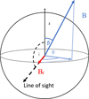 |
Fig. 1 Measurement geometry of the stellar longitudinal magnetic field. |
2.3.4 Category Q4: Magnetic field at an unspecified location
In this case, we have no geometrical information. We can thus only rely on the fact that the measured magnetic field is larger than the dipolar component and that the dipolar component is minimum at the equator, an thus,
 (16)
(16)
2.3.5 Category Q5: Magnetic field in a deeper layer
The magnetic field in the atmospheric layers of a star can be quite complex. However, the average behavior in a convective layer is an increase in density with depth, leading to an increase in the magnetic field due to equipartition scaling. We thus infer an upper limit as
 (17)
(17)
The exact depth of the magnetic field at the deeper layer Bdeep is a variable and complex matter and depends on the lines that are probed.
We thus have estimates of the equatorial dipolar magnetic field for all of our categories. The various measurement categories, grouped by quality index, are illustrated in Fig. 2, and are listed in Table 1.
2.4 Structure of the database
The database collects the dipolar equatorial magnetic field estimates for 2673 stars and ancillary information on the origin of these estimates. There is a single entry per star. The following information is listed for each star:
Main identifier of the star in SIMBAD (Simbad_ID)1.
Best-quality index of available magnetic field measurements (Qn+).
Descriptive tag from Table 1.
Estimate of its equatorial magnetic field Bdip,eq, which is the median value of the values derived from the best-quality index.
Number of individual estimates entering in the above median (N_est).
Estimate type: direct, lower limit, or upper limit (T_est).
Type of information available in the literature (e.g., dipolar magnetic field at the equator, longitudinal field, magnetic field at deep layers, etc.).
Bibliographic codes of the source papers providing the measurements for the star considered.
DOI of the corresponding publications.
As the Vizier catalog library2 only accepts value-added databases and no compilation of existing catalogs, the original measurements are not duplicated in the database. The bibliographic codes can be entered in Vizier to retrieve these original measurements. Several bibliographic sources and thus several comments can be associated with a single entry. Table 2 lists the first entries of the database. The database is fully available online.
For each star, the retained estimate of equatorial magnetic field is that of the best-quality index. If several measures of this quality index are available, the median of these values is retained. This may flatten some temporal variations, which are not the main focus of our work, since many stars in this database lack enough measurement for such a study. However, to give an idea of the variability, for AD Leo, one of the most recurrent stars of our database with eight measures, including five of quality Q2, the ratio of the median absolute deviation and the median is 17.5%.
3 Inferring unmeasured stellar dipolar magnetic fields
3.1 Other physical parameters used in the inferences
Beyond using the values estimated in the database, we wished to use it to predict the dipolar magnetic field at first order of any given star for which standard stellar parameters are available. While studying SPI and associated radio emissions, Mauduit (2024) noted the correlation of the stellar magnetic field with the stellar mass and effective temperature for low-mass stars. We use these relevant parameters and additional parameters below.
The stellar mass M can be retrieved from nine existing catalogs (Muirhead et al. 2018; Hardegree-Ullman et al. 2023; Wang et al. 2024; Casagrande et al. 2011; Queiroz et al. 2023; Kordopatis et al. 2023; Kervella et al. 2022; Stassun et al. 2018; Hirsch et al. 2021). When several measurements exist for the same star, we used their median value. We also collected several other parameters that are easily accessible from SIMBAD: the effective temperature Teff, the rotation period Prot or the rotational velocity, which allowed us to constrain the rotation period, the age A, the V-band magnitude V, and the stellar diameter D. By studying the inter-correlations between these parameters (see Appendix A), we found that the mass and diameter are strongly inter-correlated and are thus redundant parameters, and so are the effective temperature and the V-band magnitude. It is nevertheless useful to retain all these parameters in a catalog because no parameter is measured for all stars, so redundant parameters can be used instead when available.
Figure 3 displays scatter plots between Bdip,eq and each of the above stellar parameters. No simple relation appears in these diagrams, but some v-shaped structure that peaks at around 1Msun and 5000 K, is present in panels Bdip,eq(M) and Bdip,eq(Teff), respectively, suggesting that the parameters M and Teff contain relevant information about Bdip. To a lesser extent, this is also the case for the rotation period Prot with a decreasing tendency. By contrast, the dipolar magnetic field does not seem to be related to the stellar age. It is clear that none of these parameters alone is sufficient to infer Bdip, but a combination of parameters could carry enough information to make relevant predictions.
 |
Fig. 2 Categorization of stellar magnetic field measurements, grouped by quality index. |
First lines of the database.
3.2 K-nearest neighbors method
The K-nearest neighbors (KNN) method (Fix 1985) is based on the assumption that in a set of points characterized by intercorrelated parameters, the value of a given parameter is likely similar to the values of that parameter taken by neighboring points in the multidimensional space where each parameter corresponds to one dimension. In other words, similar values for some parameters are likely to imply similar values for another parameter, namely Bdip,eq.
We thus built a multidimensional space where each parameter Pi took values along one axis. Each point (i.e., each star) in the catalog had a position in this space, possibly with undefined values along some axes (corresponding to unknown values for the corresponding parameters). For a given star a with parameters (Pia), the KNN estimate of its dipolar magnetic field is the distance-weighted mean of the dipolar magnetic field of the K-nearest stars in this space, according to a Cartesian metric,
 (18)
(18)
where Δab is the distance between star a and star b.
As this method is only valid when applied to a catalog for which the value of each parameter is known for each star, it implies that the subcatalog from the catalog that can be used for a given estimation depends on the selection of the parameters considered. We do not know a priori the best set of parameters to use among (M, Teff, P, A, V, D), but the study by Mauduit (2024) and the analysis of the parameter redundancy (Appendix A) showed that the stellar mass and the effective temperature are two important parameters for characterizing the magnetic field. After some testing, we selected seven sets of parameters detailed in Table 3, each of them containing at least the stellar mass M or the effective temperature Teff. We did not explore all possible combinations of parameters because of the redundancies mentioned above.
It is important to note that the stars used in a given parameter set for the KNN method must have measurements of all the parameters of the set. Thus, each parameter set corresponds to a different subcatalog of stars from our catalog. Sets counting many parameters naturally lead to sparser subcatalogs than sets counting one or few parameters (see Table 3).
We measured the relevance of each parameter set for estimating Bdip,eq by defining the score S,
 (19)
(19)
where Bdip,meas is the value Bdip,eq listed in our catalog, Bdip,KNN is its estimate obtained with the KNN method, MAD() is the median absolute deviation estimator, a robust estimator of the standard deviation less sensitive to outliers, and f is the normalization function (based on a logarithm) detailed in Appendix B.1. The score S should tend toward 1 if the KNN prediction is perfect, and toward 0 or a negative value if it is poorer than just taking the average value of the sampled Bdip,eq around the evaluation point. We computed this score for each parameter set listed in Table 3.
We noted that three parameter sets have a higher score than the set that included all six stellar parameters, which appears itself relevant with a score of 0.56. This confirms that selecting a sparser set of relevant parameters leads to a more efficient estimation of Bdip,eq than including redundant parameters. This may be explained in two ways: one or several parameters may be irrelevant for determining Bdip,eq, and they thus pollute the estimation. Alternatively, this might be due to the much smaller size of the subcatalog of stars for which all six parameters are measured compared to subcatalogs of stars for which only M, Prot, and Teff are known (see Table 3). This also confirms the idea that D and V strongly depend on M and Teff, respectively (from known stellar scaling laws, e.g. Eker et al. 2018; Flower 1996), and that we do not need to expand the diversity of the parameter sets to consider further.
From this point, the application of the KNN method is simple: for a given star with known parameters (Pi), we used the KNN fit for the parameter set with best score S that was included in (Pi). For example, when we only knew Mi, Prot,i, and Vi, we used the KNN method with the parameter set (M, Prot), which has a score S = 0.80. When we also knew Teff,i, we instead used the parameter set (M, Prot, Teff), which has a score S = 0.84. It is worth noting that the set (M, Prot, A, Teff, D, V) was never used because whenever we had access to all these parameters, we used our best set, (M, Prot, Teff).
For each set of parameters, we calculated the minimum and maximum values for each parameter in our catalog to establish the valid range for which the KNN method could be applied. Consequently, when a star has a parameter measurement outside the corresponding validity range, we did not use this set. When the parameter was outside of the validity range for all sets, we were unable to use the KNN method to perform a prediction.
In summary, to predict the dipolar magnetic field of a given star, we used the set of parameters with the best score S that contained the measured parameters of the star within their validity range. We applied the KNN method fit on the data available in this set of parameters.
To test the KNN method, we predicted the magnetic field of each star of the catalog with it for which we had an observational estimate of Bdip,eq. We applied the KNN method to the entire catalog except for that star. We obtained the estimates displayed in Fig. 4, which shows that we successfully predicted the main trend of the catalog. However, the distribution is relatively broad and noisy, and the lower values tend to be slightly overestimated, while the higher values are slightly underestimated. This is typical of the behavior of KNN predictions when a relevant parameter is missing or the noise is high (Cover & Hart 1967). We deduce from this that while we have useful parameters for predicting a stellar magnetic field, these results suggest that a relevant parameter is still missing from the analysis. Hubrig et al. (2013) mentions, for example, that fossil fields might appear for high-mass stars, or that mass transfer might perturb the magnetic field for close binaries. The situations are various and complex, and the missing parameter(s) can be extrinsic to the observed stars.
Using the data from Fig. 4, we estimated the error ratio EKNN, computed as
 (20)
(20)
The distribution of this error is well fit by a Gaussian function (Fig. 5) with average ~0 and standard deviation 0.63. Since this is a logarithmic error, this means that Bdip,eq is correctly estimated on average (without a systematic bias), but the 1σ uncertainty is a factor of 100.63 ≃ 4 (the 3σ uncertainty is equal to a factor 76).
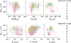 |
Fig. 3 Dipolar equatorial magnetic field Bdip,eq as a function of the other stellar parameters (mass, effective temperature, rotation period, age, V-band magnitude, and diameter). |
Parameter sets used with the KNN method applied to our catalog, sorted by their relevance score.
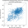 |
Fig. 4 Values of Bdip,eq computed by the KNN method versus their actual measures. The dashed line indicates the first bisector. Notes. Low Bdip,eq are mostly above the dashed line, and thus overestimated, while the bulk of high values (dark blue region) are slightly underestimated. |
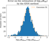 |
Fig. 5 Distribution of errors of the KNN method, fitted by a Gaussian function. Notes. The offset of the Gaussian is –0.006, and its standard deviation is 0.63. |
3.3 Neural network method
The performance of the KNN algorithm described in the previous section relies heavily on the selection of the most relevant subset of parameters (see Table 3). However, recent advances in machine learning enable the development of a neural network (NN) model that can effectively capture the data complexity without requiring explicit parameter selection. The NN was trained on a representative subset of the data (approximately 80% of the catalog), with the goal of modeling the complex relations among the parameters.
A first attempt was made with a single small linear and dense network composed of three layers of eight neurons. The network entries were the stellar parameters (Pi) for each star, and the output was the estimated dipolar magnetic field Bdip,eqi. We defined a training set composed of a random selection covering 80% of the stars from the catalog, and a validation set with the remaining 20%. The network was then trained iteratively on the training set, using the minimum square error between estimated and measured Bdip,eq as the loss function. This first attempt revealed a strong bias for high values of Bdip,eq: magnetic field estimates above 100 G were lower by one to two orders of magnitude than the measured values. The limitation of this training was the presence of gaps in the parameter space (due to missing measurements) and the relatively small size of the training set of about 330 stars.
Thus, we undertook a second approach and modified the architecture of the network to account for the slope change around 102 G. As explained in Appendix B.3, we used a restricted form of a mixture of experts (MoE) network composed of two linear networks and a scalar mixture of the network outputs to obtain a more precise and smoother inference adapted to both regimes (Jacobs et al. 1991). The data were transformed in logarithmic scale for normalization reasons, as detailed in Appendix B.1. The loss function was combined with a (learned) weighting factor α to smoothly transition between the two expert regimes. The training proceeded over 250 epochs, after which the validation loss reached a plateau. Then, we ran the network on the validation set to obtain the values shown in Fig. 6. These values show a moderate correlation, with a Pearson coefficient of 0.67.
The distribution is generally well centered around the bisector. However, the highest values of Bdip,eq,NN remain underestimated, despite attempts to optimize the neural network hyperparameters (see Appendix B.3). This underestimation may result from insufficient training data needed to represent all subpopulations, or from missing parameters that are important for understanding the origin of strong stellar magnetic fields.
We again computed an error ratio ENN similar as the above,
 (21)
(21)
which follows the distribution presented in Fig. 7. We repeated this operation for 100 different randomly drawn validation sets, each of them representing 10% of the full catalog, and we fit a Gaussian function to the distribution of the errors for each of them. The centroid and standard deviation of each fit are plotted in Fig. 8. The error distribution, and thus, the predictions, are quite stable. The centroid is 0.02 ± 0.05, which is fully compatible with zero within the uncertainty, and the standard deviation of the Gaussian fit is 0.59 ± 0.03. This yields an overall uncertainty for the NN estimates of  .
.
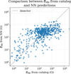 |
Fig. 6 Values of Bdip,eq computed by the neural network versus the actual measurements for the validation set. |
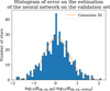 |
Fig. 7 Error distribution of the NN method, fitted by a Gaussian function. Notes. Gaussian centroid (0.02) and its standard deviation (0.58). |
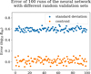 |
Fig. 8 Centroid and standard deviation of the Gaussian fit for 100 runs with different random validation sets. Notes. Median centroid (0.02) and the median standard deviation (0.59). |
3.4 Comparison between the KNN and NN methods
We found that both methods provide estimates of the logarithmic ratio of estimated and predicted Bdip,eq with similar uncertainties: ~0.63 for the KNN method, and ~0.59 for the NN method. However, because the KNN approach reproduces the highest magnetic field values (above 100 G) better, we chose it as the preferred method. A limitation of the KNN approach is that it can be restrictive in the range of stellar parameters it accepts as input. For instance, if a star lies outside the validity interval of all available parameter sets, the KNN method cannot produce a reliable estimate. In contrast, the neural network can still provide a prediction. Therefore, when estimating the stellar equatorial dipolar magnetic field, we used the KNN method whenever its validity conditions were met, and we resorted to the neural network only when KNN could not be applied.
4 Discussion and conclusion
We presented two model-agnostic methods to provide estimates of stellar magnetic fields from available measurements of other stellar parameters. The similar level of uncertainties found for these two entirely independent methods might mean that we reach the limit of information that can be derived from a general and intrinsic parameters-based approach and the available data. As mentioned above, the behavior of the KNN method shows that the mass M and rotation period Prot are relevant information for predicting the large-scale stellar magnetic field Bdip,eq. Stellar parameters that are strongly correlated with M or Prot, such as the effective temperature Teff, can serve as proxies when the primary parameters are unavailable. The KNN results also suggest that the stellar parameters we considered (i.e., M, Prot, A, Teff, D, and V) may not fully capture the relevant physics of stellar magnetism, and that additional parameters of comparable importance might be missing from the analysis. Increasing the validity interval of the key magnetic field parameters M, P and Teff (see Table 3) is likely to reduce the uncertainties in our estimates. More measures of stellar magnetic fields for more stars would also reduce uncertainties because the lack of values is likely an important contribution to the noise. It is important to note that our approach is relatively simple: no physical stellar model or simulation is used in order to predict a magnetic field as the result, for instance, of stellar convection or other complex and not fully understood mechanisms. Our approach is data focused and relies on the most accessible stellar parameters and the direct or indirect magnetic field measurements that we aggregated in our catalog. No assumption is made on the physical mechanisms underlying the relations between stellar parameters, and thus, we do not claim to produce any model, but only to provide constraints for future models, and especially, numerical estimates of stellar magnetic field values.
We have built a stellar magnetic field database from measurements collected from the literature, making these measurements commensurable by deducing from them a single estimator, the dipolar magnetic field at equator Bdip,eq (see Table 2). This database will be available via the Vizier catalog library3. We used this database to infer relations between large-scale stellar magnetic fields and other easily accessible stellar parameters. Our approach is data focused and uses no model a priori, but a K-nearest neighbors (KNN) method and a neural network (NN) method to extrapolate from measured values. The KNN method is to be preferred whenever possible. Our results show that the stellar mass, the rotation period, and the effective temperature are relevant parameters for characterizing the magnetic field, but they do not contain all the relevant information. The prediction models will be available online in a repository4.
Following this work, our database and the associated extrapolation methods will be used to improve the reliability of ensemble predictions of radio emissions from exoplanetary magnetospheres and star-planet interactions, such as those of the PALANTIR model (Mauduit et al. 2023; Mauduit 2024, 2025). In these models, the dipolar stellar magnetic field is a crucial (it determines the magnetic field of the stellar wind) but sparsely known parameter.
Data availability
Table 2 is fully available at the CDS via https://cdsarc.cds.unistra.fr/viz-bin/cat/J/A+A/710/A16.
Acknowledgements
We thank the referee for their comments during the revision process. We thank Claude Catala for discussions of ZDI measurements and their interpretation, and Benoit Semelin and Fadi Nammour for their advices on the neural network method. The authors acknowledge funding from the ERC under the European Union’s Horizon 2020 research and innovation programme (grant agreement no. 101020459 - Exoradio).
References
- Babcock, H. W. 1958, ApJS, 3, 141 [Google Scholar]
- Bagnulo, S., & Landstreet, J. D. 2015, in Polarimetry of Stars and Planetary Systems, eds. L. Kolokolova, J. Hough, & A.-C. Levasseur-Regourd (Cambridge: Cambridge University Press), 224 [Google Scholar]
- Bagnulo, S., Fossati, L., Landstreet, J. D., & Izzo, C. 2015, A&A, 583, A115 [NASA ADS] [CrossRef] [EDP Sciences] [Google Scholar]
- Berger, E. 2006, ApJ, 648, 629 [NASA ADS] [CrossRef] [Google Scholar]
- Brown, E. L., Jeffers, S. V., Marsden, S. C., et al. 2022, MNRAS, 514, 4300 [CrossRef] [Google Scholar]
- Callingham, J. R., Pope, B. J. S., Kavanagh, R. D., et al. 2024, Nat. Astron., 8, 1359 [NASA ADS] [CrossRef] [Google Scholar]
- Casagrande, L., Schönrich, R., Asplund, M., et al. 2011, A&A, 530, A138 [NASA ADS] [CrossRef] [EDP Sciences] [Google Scholar]
- Cover, T., & Hart, P. 1967, IEEE Trans. Inform. Theory, 13, 21 [CrossRef] [Google Scholar]
- Donati, J.-F., Brown, S. F., Semel, M., et al. 1992, A&A, 265, 682 [NASA ADS] [Google Scholar]
- Donati, J.-F., Morin, J., Petit, P., et al. 2008, MNRAS, 390, 545 [NASA ADS] [CrossRef] [Google Scholar]
- Donati, J.-F., Cristofari, P. I., Finociety, B., et al. 2023, MNRAS, 525, 455 [NASA ADS] [CrossRef] [Google Scholar]
- Eker, Z., Bak⅛ V., Bilir, S., et al. 2018, MNRAS, 479, 5491 [NASA ADS] [CrossRef] [Google Scholar]
- Fix, E. 1985, Discriminatory Analysis: Nonparametric Discrimination, Consistency Properties (Texas: USAF School of Aviation Medicine) [Google Scholar]
- Flower, P. J. 1996, ApJ, 469, 355 [NASA ADS] [CrossRef] [Google Scholar]
- Folsom, C. P., Ó Fionnagáin, D., Fossati, L., et al. 2020, A&A, 633, A48 [NASA ADS] [CrossRef] [EDP Sciences] [Google Scholar]
- Hardegree-Ullman, K. K., Apai, D., Bergsten, G. J., Pascucci, I., & López-Morales, M. 2023, AJ, 165, 267 [NASA ADS] [CrossRef] [Google Scholar]
- Hirsch, L. A., Rosenthal, L., Fulton, B. J., et al. 2021, AJ, 161, 134 [NASA ADS] [CrossRef] [Google Scholar]
- Hubrig, S., Schöller, M., Ilyin, I., et al. 2013, A&A, 551, A33 [CrossRef] [EDP Sciences] [Google Scholar]
- Jacobs, R. A., Jordan, M. I., Nowlan, S. J., & Hinton, G. E. 1991, Neural Comput., 3, 79 [Google Scholar]
- Kervella, P., Arenou, F., & Thévenin, F. 2022, A&A, 657, A7 [NASA ADS] [CrossRef] [EDP Sciences] [Google Scholar]
- Kordopatis, G., Schultheis, M., McMillan, P. J., et al. 2023, A&A, 669, A104 [NASA ADS] [CrossRef] [EDP Sciences] [Google Scholar]
- Lang, K. R. 2006, Sun, Earth and Sky (Berlin: Springer) [Google Scholar]
- Mauduit, E. 2024, Theses, Université PSL Paris Sciences & Lettres (PSL Research University), France [Google Scholar]
- Mauduit, E. 2025, EmilieMauduit/PALANTIR: Release v0.1.1 [Google Scholar]
- Mauduit, E., Grießmeier, J.-M., Zarka, P., & Turner, J. D. 2023, in Planetary, Solar and Heliospheric Radio Emissions IX, eds. C. K. Louis, C. M. Jackman, G. Fischer, A. H. Sulaiman, & P. Zucca (Dublin: Dublin Institute for Advanced Studies), 103092 [Google Scholar]
- Mestel, L. 1968, MNRAS, 138, 359 [NASA ADS] [CrossRef] [Google Scholar]
- Morin, J., Donati, J.-F., Petit, P., et al. 2008, MNRAS, 390, 567 [Google Scholar]
- Muirhead, P. S., Dressing, C. D., Mann, A. W., et al. 2018, AJ, 155, 180 [NASA ADS] [CrossRef] [Google Scholar]
- Preston, G. W. 1967, ApJ, 150, 547 [NASA ADS] [CrossRef] [Google Scholar]
- Queiroz, A. B. A., Anders, F., Chiappini, C., et al. 2023, A&A, 673, A155 [NASA ADS] [CrossRef] [EDP Sciences] [Google Scholar]
- Semel, M. 1989, A&A, 225, 456 [NASA ADS] [Google Scholar]
- Stassun, K. G., Oelkers, R. J., Pepper, J., et al. 2018, AJ, 156, 102 [Google Scholar]
- Stibbs, D. W. N. 1950, MNRAS, 110, 395 [Google Scholar]
- Wang, Y., Zhang, L., Su, T., Han, X. L., & Misra, P. 2024, A&A, 686, A164 [NASA ADS] [CrossRef] [EDP Sciences] [Google Scholar]
- Weber, E. J., & Davis, Jr., L. 1967, ApJ, 148, 217 [NASA ADS] [CrossRef] [Google Scholar]
- Zarka, P. 2007, Planet. Space Sci., 55, 598 [Google Scholar]
- Zarka, P. 2018, in Handbook of Exoplanets, eds. H. J. Deeg & J. A. Belmonte (Berlin: Springer), 22 [Google Scholar]
- Zarka, P., Treumann, R. A., Ryabov, B. P., & Ryabov, V. B. 2001, Ap&SS, 277, 293 [NASA ADS] [CrossRef] [Google Scholar]
Appendix A Inter-correlation studies using the variance inflation factor
We used the variance inflation factor (VIF) to determine the redundancies among stellar parameters in the catalog. In a given set of N parameters (Pi), the VIF is a measure of inter-correlation between each parameter and the others. For each parameter Pi, it is computed via a least square regression to determine the best expression of each parameter Pi as a linear combination of the N − 1 other parameters (Pj, j ≠ i):
 (A.1)
(A.1)
with {aj} constants, and ε the residual. For each regression we obtain a coefficient of determination R2i (which is the square of the Pearson correlation coefficient between the observed and modeled values of Pi). The VIF for the parameter Pi is
 (A.2)
(A.2)
The higher the VIF, the stronger the multi-colinearity between parameters. A VIF above 10 is high and indicates high intercorrelations. We studied which parameters are redundant with others by first calculating the VIF for each parameter (Pi) with all six parameters (M, Teff, Prot, A, V, D) studied together, then by removing one parameter and recalculating the VIFs for the remaining set of five parameters. For example, we observe in Table A.1 that removing the parameter “diameter” considerably reduces the VIF of the parameters “mass” and “rotation period,” but the other parameters are barely affected. We can deduce that there is a high redundancy between the diameter (D), and the stellar mass (M) and rotation period (Prot).
We find that the VIFs computed on the 6-parameters set are quite high for most parameters, which reveals high multicolinearity. Then we successively exclude one parameter and recompute the VIFs on the remaining five-parameter set. When the VIF strongly decreases, it reveals a strong correlation between the corresponding parameter and the excluded one. We conclude from Table A.1 that diameter D is highly correlated with mass M and rotation period P, but the latter two are nearly independent. Similarly, the effective temperature Teff is correlated with the mass M and V-band magnitude V, but the latter two are independent. Finally, the age A of the star seems generally uncorrelated with all other stellar parameters listed in the catalog.
VIF values for the set of six parameters (first line), and for the six sets of five parameters (next six lines).
Appendix B Details on the KNN and the neural network methods
Appendix B.1 Parameter normalization
For the KNN and the neural network methods, we use the base-10 logarithm of the values, so that larger values do not weight more and have the same granularity as smaller values. We also normalize the different parameters so that none of them has more weight than others because of a choice of units. To avoid pollution by outliers, we finally range the (log10 of the) parameter values between 0 and 1, with 0 corresponding to the first decile of the parameter’s distribution log10(P10%), and 1 to the ninth decile log10(P90%). So, for the parameter (P) of a given star (k):
 (B.1)
(B.1)
with
 (B.2)
(B.2)
 (B.3)
(B.3)
Appendix B.2 Hyper-parameters of the KNN method
The main hyper-parameters of the K nearest neighbor method is K, the number of neighbors taken into account, and the choice of the metric. As mentioned above, we use a Cartesian metric. It is straightforward and our problem doesn’t seem to require a more sophisticated metric.
To determine the best value of K for each stellar parameters set, we randomly draw a fitting set of a third of the corresponding subcatalog, and a test set made of the rest of the subcatalog. We apply the KNN method for each parameter set, and for each integer value of K from 2 to 10, to the test catalogs. Finally we use the scoring system defined in Sect. 3.2 to evaluate the quality of the estimates. For each parameter set, we retain the value of K giving the best score, as listed table B.1. Thes are the K values used in Sect. 3.2 with each parameter set.
Number of first neighbors (K) that provide the best KNN estimates of Bdip,eq for each parameter set.
Appendix B.3 Hyper-parameters of the neural network method
The architecture of the neural network is a simplified version of the “Mixture of Experts” (MoE) network, with two experts being trained in parallel (as illustrated in Fig. B.1). It actually consists of three subnetworks: two “expert” subnetwork (A and B) and one “gating” network to combine the result of the two experts. Each expert network is a linear neural network composed of two 16-neuron layers linked using ReLU activation functions (rectified linear unit, defined as the non-negative part of its argument), then an output layer of only one neuron with a linear activation function. A third network composed of one dense layer of 16 neurons (with ReLU) and a single neuron dense layer with a sigmoid activation function. The purpose of each expert is to learn the behavior of the dataset in a given [Bmin, Bmax] domain for each expert. The role of the third layer is to capture the two different regimes identified around Bdip,eq ~ 102 G and combine them linearly to provide the final output Bdip,eq. The learned “g” factor is the relative weight of the inferences produced by expert A and B, allowing a smooth transitioning between the two regimes. After training, each expert is able to infer in its specific domain that is defined by the training of g, which is the equivalent of defining a smooth boundary.
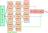 |
Fig. B.1 Architecture of the neural network used to estimate Bdip,eq from other stellar parameters. |
The network is trained over 250 epochs, by batches of 64 points, with an histogram-weighted mean square error as the loss function. Each data point is weighted relatively to the representative fraction of its corresponding bin in a normalized histogram. This enables to give an equitable representation of each bin to the network, independent of large variations of B (which can range from 10−1 to 104). A number of M bins (in log scale) has been chosen to slice the dynamic range of the dataset. We made the choice to keep a small number of layers and of neurons because of the relatively small size of our catalog. Missing values in the data are replaced using a KNN imputer, which issues likely values considering other stellar parameters. The choice of the network parameters was made empirically via trials and errors on a subset of the catalog.
All Tables
Different categories of ZDI magnetic field measurements found in the literature and included in the database, with their associated descriptive tag and quality index.
Parameter sets used with the KNN method applied to our catalog, sorted by their relevance score.
VIF values for the set of six parameters (first line), and for the six sets of five parameters (next six lines).
Number of first neighbors (K) that provide the best KNN estimates of Bdip,eq for each parameter set.
All Figures
|
Fig. 1 Measurement geometry of the stellar longitudinal magnetic field. |
| In the text | |
|
Fig. 2 Categorization of stellar magnetic field measurements, grouped by quality index. |
| In the text | |
|
Fig. 3 Dipolar equatorial magnetic field Bdip,eq as a function of the other stellar parameters (mass, effective temperature, rotation period, age, V-band magnitude, and diameter). |
| In the text | |
|
Fig. 4 Values of Bdip,eq computed by the KNN method versus their actual measures. The dashed line indicates the first bisector. Notes. Low Bdip,eq are mostly above the dashed line, and thus overestimated, while the bulk of high values (dark blue region) are slightly underestimated. |
| In the text | |
|
Fig. 5 Distribution of errors of the KNN method, fitted by a Gaussian function. Notes. The offset of the Gaussian is –0.006, and its standard deviation is 0.63. |
| In the text | |
|
Fig. 6 Values of Bdip,eq computed by the neural network versus the actual measurements for the validation set. |
| In the text | |
|
Fig. 7 Error distribution of the NN method, fitted by a Gaussian function. Notes. Gaussian centroid (0.02) and its standard deviation (0.58). |
| In the text | |
|
Fig. 8 Centroid and standard deviation of the Gaussian fit for 100 runs with different random validation sets. Notes. Median centroid (0.02) and the median standard deviation (0.59). |
| In the text | |
|
Fig. B.1 Architecture of the neural network used to estimate Bdip,eq from other stellar parameters. |
| In the text | |
Current usage metrics show cumulative count of Article Views (full-text article views including HTML views, PDF and ePub downloads, according to the available data) and Abstracts Views on Vision4Press platform.
Data correspond to usage on the plateform after 2015. The current usage metrics is available 48-96 hours after online publication and is updated daily on week days.
Initial download of the metrics may take a while.