| Issue |
A&A
Volume 710, June 2026
|
|
|---|---|---|
| Article Number | A27 | |
| Number of page(s) | 18 | |
| Section | Planets, planetary systems, and small bodies | |
| DOI | https://doi.org/10.1051/0004-6361/202659419 | |
| Published online | 02 June 2026 | |
Euclid: Asteroid rotation periods from the Euclid Ecliptic Survey★
1
Institute of Physics, Laboratory of Astrophysics, Ecole Polytechnique Fédérale de Lausanne (EPFL), Observatoire de Sauverny,
1290
Versoix,
Switzerland
2
ESAC/ESA, Camino Bajo del Castillo, s/n, Urb. Villafranca del Castillo,
28692
Villanueva de la Cañada, Madrid,
Spain
3
Department of Physics,
PO Box 64, University of Helsinki,
00014
Helsinki,
Finland
4
European Southern Observatory,
Karl-Schwarzschild-Str. 2,
85748
Garching,
Germany
5
Instituto de Astrofísica de Canarias,
38205
La Laguna, Tenerife,
Spain
6
Asteroid Engineering Laboratory, Luleå University of Technology,
Box 848,
98128
Kiruna,
Sweden
7
Department of Mathematics and Physics E. De Giorgi, University of Salento, Via per Arnesano, CP-I93,
73100
Lecce,
Italy
8
INFN, Sezione di Lecce, Via per Arnesano, CP-193,
73100
Lecce,
Italy
9
INAF-Sezione di Lecce, c/o Dipartimento Matematica e Fisica, Via per Arnesano,
73100
Lecce,
Italy
10
Université Côte d’Azur, Observatoire de la Côte d’Azur, CNRS, Laboratoire Lagrange, Bd de l’Observatoire, CS 34229,
06304
Nice cedex 4,
France
11
European Space Agency/ESRIN,
Largo Galileo Galilei 1,
00044
Frascati, Roma,
Italy
12
Université de Franche-Comté, Institut UTINAM, CNRS UMR6213, OSU THETA Franche-Comté-Bourgogne, Observatoire de Besançon,
BP 1615,
25010
Besançon Cedex,
France
13
Max Planck Institute for Extraterrestrial Physics,
Giessenbachstr. 1,
85748
Garching,
Germany
14
Mullard Space Science Laboratory, University College London, Holmbury St Mary, Dorking,
Surrey
RH5 6NT,
UK
15
Institute for Astronomy, University of Edinburgh, Royal Observatory, Blackford Hill,
Edinburgh
EH9 3HJ,
UK
16
Oskar Klein Centre for Cosmoparticle Physics, Department of Physics, Stockholm University,
Stockholm
106 91,
Sweden
17
FRACTAL S.L.N.E.,
calle Tulipán 2, Portal 13 1A,
28231,
Las Rozas de Madrid,
Spain
18
Kapteyn Astronomical Institute, University of Groningen,
PO Box 800,
9700
AV
Groningen,
The Netherlands
19
Universidad de La Laguna, Dpto. Astrofísica,
38206
La Laguna, Tenerife,
Spain
20
Centro de Astrobiología (CAB), CSIC-INTA, ESAC Campus, Camino Bajo del Castillo s/n,
28692
Villanueva de la Cañada, Madrid,
Spain
21
Leiden Observatory, Leiden University,
Einsteinweg 55,
2333
CC
Leiden,
The Netherlands
22
INAF – Osservatorio Astronomico di Brera,
Via Brera 28,
20122
Milano,
Italy
23
IFPU, Institute for Fundamental Physics of the Universe,
via Beirut 2,
34151
Trieste,
Italy
24
INAF – Osservatorio Astronomico di Trieste,
Via G. B. Tiepolo 11,
34143
Trieste,
Italy
25
INFN, Sezione di Trieste,
Via Valerio 2,
34127
Trieste
TS,
Italy
26
SISSA, International School for Advanced Studies,
Via Bonomea 265,
34136
Trieste
TS,
Italy
27
Dipartimento di Fisica e Astronomia, Università di Bologna,
Via Gobetti 93/2,
40129
Bologna,
Italy
28
INAF – Osservatorio di Astrofisica e Scienza dello Spazio di Bologna,
Via Piero Gobetti 93/3,
40129
Bologna,
Italy
29
INFN – Sezione di Bologna,
Viale Berti Pichat 6/2,
40127
Bologna,
Italy
30
INAF – Osservatorio Astronomico di Padova,
Via dell’Osservatorio 5,
35122
Padova,
Italy
31
Dipartimento di Fisica, Università di Genova,
Via Dodecaneso 33,
16146,
Genova,
Italy
32
INFN – Sezione di Genova,
Via Dodecaneso 33,
16146
Genova,
Italy
33
Department of Physics “E. Pancini”, University Federico II,
Via Cinthia 6,
80126,
Napoli,
Italy
34
INAF – Osservatorio Astronomico di Capodimonte,
Via Moiariello 16,
80131
Napoli,
Italy
35
Dipartimento di Fisica, Università degli Studi di Torino,
Via P. Giuria 1,
10125
Torino,
Italy
36
INFN – Sezione di Torino,
Via P. Giuria 1,
10125
Torino,
Italy
37
INAF – Osservatorio Astrofisico di Torino,
Via Osservatorio 20,
10025
Pino Torinese (TO),
Italy
38
INAF-IASF Milano,
Via Alfonso Corti 12,
20133
Milano,
Italy
39
Centro de Investigaciones Energéticas, Medioambientales y Tecnológicas (CIEMAT),
Avenida Complutense 40,
28040
Madrid,
Spain
40
Port d’Informació Científica, Campus UAB, C. Albareda s/n,
08193
Bellaterra (Barcelona),
Spain
41
Institut d’Estudis Espacials de Catalunya (IEEC), Edifici RDIT, Campus UPC,
08860
Castelldefels, Barcelona,
Spain
42
Institute of Space Sciences (ICE, CSIC), Campus UAB, Carrer de Can Magrans, s/n,
08193
Barcelona,
Spain
43
INAF-Osservatorio Astronomico di Roma,
Via Frascati 33,
00078
Monteporzio Catone,
Italy
44
INFN section of Naples,
Via Cinthia 6,
80126
Napoli,
Italy
45
Institute for Astronomy, University of Hawaii,
2680 Woodlawn Drive,
Honolulu,
HI
96822,
USA
46
Dipartimento di Fisica e Astronomia “Augusto Righi” – Alma Mater Studiorum Università di Bologna,
Viale Berti Pichat 6/2,
40127
Bologna,
Italy
47
Jodrell Bank Centre for Astrophysics, Department of Physics and Astronomy, University of Manchester,
Oxford Road,
Manchester
M13 9PL,
UK
48
Université Claude Bernard Lyon 1, CNRS/IN2P3, IP2I Lyon,
UMR 5822,
Villeurbanne
69100,
France
49
Institut de Ciències del Cosmos (ICCUB), Universitat de Barcelona (IEEC-UB),
Martí i Franquès 1,
08028
Barcelona,
Spain
50
Institució Catalana de Recerca i Estudis Avançats (ICREA),
Passeig de Lluís Companys 23,
08010
Barcelona,
Spain
51
Institut de Ciencies de l’Espai (IEEC-CSIC), Campus UAB, Carrer de Can Magrans, s/n Cerdanyola del Vallés,
08193
Barcelona,
Spain
52
UCB Lyon 1, CNRS/IN2P3, IUF, IP2I Lyon,
4 rue Enrico Fermi,
69622
Villeurbanne,
France
53
Department of Astronomy, University of Geneva,
ch. d’Ecogia 16,
1290
Versoix,
Switzerland
54
Université Paris-Saclay, CNRS, Institut d’astrophysique spatiale,
91405
Orsay,
France
55
INAF-Istituto di Astrofisica e Planetologia Spaziali,
via del Fosso del Cavaliere, 100,
00100
Roma,
Italy
56
University Observatory, LMU Faculty of Physics,
Scheinerstr. 1,
81679
Munich,
Germany
57
Universitäts-Sternwarte München, Fakultät für Physik, Ludwig-Maximilians-Universität München,
Scheinerstr. 1,
81679
München,
Germany
58
Institute of Theoretical Astrophysics, University of Oslo,
PO Box 1029 Blindern,
0315
Oslo,
Norway
59
Jet Propulsion Laboratory, California Institute of Technology,
4800 Oak Grove Drive,
Pasadena,
CA
91109,
USA
60
Department of Physics, Lancaster University,
Lancaster
LA1 4YB,
UK
61
Felix Hormuth Engineering,
Goethestr. 17,
69181
Leimen,
Germany
62
Technical University of Denmark,
Elektrovej 327,
2800
Kgs. Lyngby,
Denmark
63
Cosmic Dawn Center (DAWN),
Denmark
64
Max-Planck-Institut für Astronomie,
Königstuhl 17,
69117
Heidelberg,
Germany
65
NASA Goddard Space Flight Center,
Greenbelt,
MD
20771,
USA
66
Université de Genève, Département de Physique Théorique and Centre for Astroparticle Physics,
24 quai Ernest-Ansermet,
1211
Genève 4,
Switzerland
67
Helsinki Institute of Physics,
Gustaf Hällströmin katu 2, University of Helsinki,
00014
Helsinki,
Finland
68
Laboratoire d’etude de l’Univers et des phenomenes eXtremes, Observatoire de Paris, Université PSL, Sorbonne Université, CNRS,
92190
Meudon,
France
69
SKAO, Jodrell Bank, Lower Withington,
Macclesfield
SK11 9FT,
UK
70
Centre de Calcul de l’IN2P3/CNRS,
21 avenue Pierre de Coubertin
69627
Villeurbanne Cedex,
France
71
Universität Bonn, Argelander-Institut für Astronomie,
Auf dem Hügel 71,
53121
Bonn,
Germany
72
INFN-Sezione di Roma,
Piazzale Aldo Moro 2, c/o Dipartimento di Fisica, Edificio G. Marconi,
00185
Roma,
Italy
73
Aix-Marseille Université, CNRS, CNES, LAM,
Marseille,
France
74
Dipartimento di Fisica e Astronomia “Augusto Righi” – Alma Mater Studiorum Università di Bologna,
via Piero Gobetti 93/2,
40129
Bologna,
Italy
75
Department of Physics, Institute for Computational Cosmology, Durham University,
South Road,
Durham
DH1 3LE,
UK
76
Université Paris Cité, CNRS, Astroparticule et Cosmologie,
75013
Paris,
France
77
CNRS-UCB International Research Laboratory, Centre Pierre Binétruy, IRL2007, CPB-IN2P3,
Berkeley,
USA
78
Telespazio UK S.L. for European Space Agency (ESA), Camino bajo del Castillo, s/n, Urbanizacion Villafranca del Castillo, Villanueva de la Cañada,
28692
Madrid,
Spain
79
Institut de Física d’Altes Energies (IFAE), The Barcelona Institute of Science and Technology, Campus UAB,
08193
Bellaterra (Barcelona),
Spain
80
European Space Agency/ESTEC,
Keplerlaan 1,
2201
AZ
Noordwijk,
The Netherlands
81
DARK, Niels Bohr Institute, University of Copenhagen,
Jagtvej 155,
2200
Copenhagen,
Denmark
82
Waterloo Centre for Astrophysics, University of Waterloo, Waterloo,
Ontario
N2L 3G1,
Canada
83
Department of Physics and Astronomy, University of Waterloo, Waterloo,
Ontario
N2L 3G1,
Canada
84
Perimeter Institute for Theoretical Physics, Waterloo,
Ontario
N2L 2Y5,
Canada
85
Space Science Data Center, Italian Space Agency, via del Politecnico snc,
00133
Roma,
Italy
86
Institute of Space Science, Str. Atomistilor,
nr. 409 Măgurele,
Ilfov
077125,
Romania
87
Consejo Superior de Investigaciones Cientificas,
Calle Serrano 117,
28006
Madrid,
Spain
88
Dipartimento di Fisica e Astronomia “G. Galilei”, Università di Padova,
Via Marzolo 8,
35131
Padova,
Italy
89
INFN-Padova,
Via Marzolo 8,
35131
Padova,
Italy
90
Instituto de Física Teórica UAM-CSIC, Campus de Cantoblanco,
28049
Madrid,
Spain
91
Institut de Recherche en Astrophysique et Planétologie (IRAP), Université de Toulouse, CNRS, UPS, CNES,
14 Av. Edouard Belin,
31400
Toulouse,
France
92
Université St Joseph, Faculty of Sciences,
Beirut,
Lebanon
93
Departamento de Física, FCFM, Universidad de Chile, Blanco Encalada
2008,
Santiago,
Chile
94
Aix-Marseille Université, CNRS/IN2P3, CPPM,
Marseille,
France
95
Department of Physics and Helsinki Institute of Physics,
Gustaf Hällströmin katu 2, University of Helsinki,
00014
Helsinki,
Finland
96
Departamento de Física, Faculdade de Ciências, Universidade de Lisboa,
Edifício C8, Campo Grande,
1749-016
Lisboa,
Portugal
97
Instituto de Astrofísica e Ciências do Espaço, Faculdade de Ciências, Universidade de Lisboa, Tapada da Ajuda,
1349-018
Lisboa,
Portugal
98
Cosmic Dawn Center (DAWN)
99
Niels Bohr Institute, University of Copenhagen,
Jagtvej 128,
2200
Copenhagen,
Denmark
100
Universidad Politécnica de Cartagena, Departamento de Electrónica y Tecnología de Computadoras,
Plaza del Hospital 1,
30202
Cartagena,
Spain
101
Caltech/IPAC, 1200 E. California Blvd.,
Pasadena,
CA
91125,
USA
102
Aurora Technology for European Space Agency (ESA), Camino bajo del Castillo, s/n, Urbanizacion Villafranca del Castillo, Villanueva de la Cañada,
28692
Madrid,
Spain
103
Institut d’Astrophysique de Paris,
98bis Boulevard Arago,
75014
Paris,
France
104
ICL, Junia, Université Catholique de Lille, LITL,
59000
Lille,
France
105
California Institute of Technology,
1200 E California Blvd,
Pasadena,
CA
91125,
USA
106
Department of Physics and Astronomy, University of British Columbia,
Vancouver,
BC
V6T 1Z1,
Canada
★★ Corresponding author: This email address is being protected from spambots. You need JavaScript enabled to view it.
Received:
11
February
2026
Accepted:
19
March
2026
Abstract
The Euclid Ecliptic Survey was conducted during the calibration phase of the mission, from 23 to 31 December 2023, as a campaign to study Solar System objects. We used data from this survey to analyse more than 23 000 appeareances of 2321 known asteroids. Due to their high apparent angular motion relative to the background stars (5–60″ h−1), these objects appear as streaks in VIS long-exposure images. We set out to estimate their spin periods, since only 7% of them have periods published in the literature. We used multiple apertures along each streak to increase the time resolution of our light curves. Our method combines a Lomb–Scargle approach with a Markov chain Monte Carlo (MCMC) algorithm to characterise the posterior distributions. Some asteroids show multimodality in the MCMC search, indicating period aliases; in these cases, we report all aliases and their likelihoods. We validate our pipeline by comparing our fitted periods with 48 published periods, including period harmonics. We find that 44% of our periods are within 1% of those published and 98% are within 15%, and we establish that with 98% confidence the best solution can be found among the first three aliases. All reliable periods reported are in agreement with our current understanding of the spin-period distribution for asteroids. We find 16 periods below the spin barrier of 2.2 h with absolute magnitudes below 19, and thus 16 candidate super-fast rotators. We provide light curves for all 2321 objects observed and 889 high-quality periods in an open-access catalogue. The asteroids with reported periods include five Mars crossers, four Cybeles, four Hildas, three Hungarias, and 877 asteroids in other regions of the main belt. Our results represent the first batch of spin periods extracted from light curves and include the first-ever period measurements for 93% of the objects.
Key words: astronomical databases: miscellaneous / surveys / minor planets, asteroids: general
This paper is published on behalf of the Euclid Consortium.
© The Authors 2026
 Open Access article, published by EDP Sciences, under the terms of the Creative Commons Attribution License (https://creativecommons.org/licenses/by/4.0), which permits unrestricted use, distribution, and reproduction in any medium, provided the original work is properly cited.
This article is published in open access under the Subscribe to Open model. This email address is being protected from spambots. You need JavaScript enabled to view it. to support open access publication.
1 Introduction
Time-resolved photometry can reveal key asteroid properties. For principal-axis rotators, rotation appears as a periodic signature in the asteroid light curve that can be used to determine the rotation period, also known as the spin period. In turn, the spin period can help with the analysis of other physical characteristics. It can constrain asteroid surface features, since surface smoothness relates to faster spin rates (Persson & Biele 2022), as well as the internal structure, since fast rotators are thought to be monolithic, while rubble-pile asteroids with relatively short periods may suffer from rotational instabilities leading to failure modes (Pravec et al. 2002; Hirabayashi et al. 2015). The spin period can help us study the thermophysical properties and grain size of the observed asteroids (Spencer et al. 1989; Lagerros 1996; Müller & Lagerros 1998; Rozitis & Green 2011; Marciniak et al. 2019). This is relevant for interpreting the thermal infrared emissions using telescopes such as the Wide-field Infrared Survey Explorer (Wright et al. 2010) or the upcoming European Space Agency’s Near-Earth Object Mission in the Infra-Red (Conversi et al. 2024) and NASA’s Near-Earth Object Surveyor (Mainzer et al. 2023). The shape of an asteroid is influenced by its current and past spin rates (Barnouin et al. 2019), and through shape models we can connect the spin period to the mass distribution of the asteroid (Ostro et al. 1995) and to the features of any binary companions (Pravec et al. 2006; Scheeres et al. 2006). The sources of asteroid rotation, mainly past collisions and the Yarkovsky–O’Keefe–Radzievskii–Paddack (YORP) effect, can also be studied using spin-period analysis (Rubincam 2000; Pravec et al. 2002; Taylor et al. 2007; Marzari et al. 2020).
While these findings are informative at the individual level, collecting a statistically significant sample of asteroid spin periods can provide insights into the formation history of our Solar System. In particular, the asteroid main belt (MB), located between Mars and Jupiter, is relevant to understanding aspects such as the migration of the giant planets to the outer Solar System (Clement et al. 2020, and references cited therein) or the origin of near-Earth objects (Granvik et al. 2017). However, as of November 2025, periods have been published for fewer than 5% (around 50 000) of the known asteroids (Berthier et al. 2023). Of these, only about 20% of the periods that include reliability flags are considered to be of high quality. The light curve analysis required to determine the spin period often needs many high-quality data points, and the brightness variations, if subtle, can lie below the noise level of small telescopes.
In this work, we exploit the capabilities of the European Space Agency’s Euclid space telescope (Euclid Collaboration: Mellier et al. 2025) to expand our catalogue of asteroid spin periods. Although large astronomical surveys covering extensive portions of the sky have produced large amounts of asteroid data in the last decade, their observing strategies have typically yielded sparse photometry for these objects. This is the case for the Zwicky Transient Facility (Bellm et al. 2018), Pan-STARRS (Kaiser et al. 2002), and the Asteroid Terrestrial-impact Last Alert System (Tonry et al. 2018). Conversely, dense asteroid light curves that can be used to determine spin periods accurately remain relatively scarce in the literature and have never been gathered for the faintest apparent magnitudes in the range of the Euclid Visible Camera (VIS; Euclid Collaboration: Cropper et al. 2025), between 20 and 24. The observing strategy of Euclid, even if not primarily designed for asteroid science but for cosmological studies, nevertheless allows us to obtain dense photometry and to fill an unexplored gap in the asteroid population.
As is discussed by Carry (2018), during its nominal six-year mission Euclid will observe up to 150 000 Solar System objects (SSOs, which includes asteroids and comets) with extraordinary photometric stability. Since the mission will reach fainter magnitudes than previous surveys, many of these asteroids will have never been observed before. To test the potential of Euclid to find and characterise SSOs, a dedicated campaign, the Euclid Ecliptic Survey (EES), was conducted during the Euclid phase-diversity calibration (PDC) at the beginning of the mission, before the start of the Euclid Wide Survey (Euclid Collaboration: Scaramella et al. 2022). The PDC observations require thermal stability and it was decided to use the thermal stabilisation periods for three sets of dedicated observing programmes, one of which was for SSOs. During this campaign, from 23 to 31 December 2023, VIS was pointed directly at the ecliptic plane and approximately followed the average motion of the MB. This strategy allows us to extract denser, longer light curves and observe more SSOs than the nominal Euclid Wide Survey mode, which generally avoids the ecliptic plane and hence produces sparser SSO photometry. The EES used both Euclid instruments, VIS and the Near Infrared Spectrometer and Photometer (NISP; Euclid Collaboration: Jahnke et al. 2025). For the purposes of this study, we only use data from VIS; the NISP analyses including thermal data are presented in a separate publication that will include a photometric analysis followed by taxonomic classification based on the multiband photometry (Pöntinen et al. 2025, Pöntinen et al., in prep.).
Figure 1 shows the EES in context, projected in ecliptic coordinates, and Fig. 2 presents a detail of the observing strategy. In this work, we use all 148 observations collected during the EES. We use trailed sources detected by Pöntinen et al. (2025) and search for periodicity in their signal. We build upon previous research that developed semi-automated pipelines to ingest the large volume of data produced by large surveys. The work pioneered by Polishook et al. (2012) and continued by Waszczak et al. (2015) and Chang et al. (2017) applied Fourier analysis to determine the spin periods of thousands of asteroids observed by the Palomar Transient Factory. Later studies shifted towards the use of Lomb–Scargle algorithms, which are more robust to unevenly sampled time series, as is generally the case for asteroid light curves (e.g. Erasmus et al. 2021; Eglitis & Svincicka 2025). As is discussed in these papers, the survey cadences used to obtain many of the published light curves yielded sparse photometry that could not always fully constrain the period, leading to ambiguous solutions. The newest surveys, such as the Vera C. Rubin Observatory, and the more recent use of space telescopes that provide denser light curves due to their observing strategy, such as NASA’s TESS and K2, have been shown to significantly improve previous spin-period estimates; for instance, the studies of Szabó et al. (2022), Sergeyev et al. (2025), Vavilov & Carry (2025), or Greenstreet et al. (2026). Our work complements these efforts and paves the way for future analyses during the Euclid Wide Survey.
The remainder of the paper is structured in five parts. Section 2 describes the data products that we used for our analysis. In Sect. 3, we develop the mathematical expressions and physical assumptions we made to construct the model for our asteroid light curves. In Sect. 4 we explain our methodology and justify any technical decisions. In Sect. 5, we present and discuss the results obtained during the validation of our pipeline and include tables with our fitted periods. Lastly, in Sect. 6, we lay out the main conclusions of our study and comment on future work.
 |
Fig. 1 Position in ecliptic co-ordinates of the EES (encircled in white) in the context of the DR1 (coloured tiles), projected using the Euclid Survey System (Gómez-Alvarez et al. 2018). The survey took place from 23 to 31 December 2023 and lay on the ecliptic plane, since it was designed to approximately follow the motion of the asteroids in the MB. A detail of the survey can be seen in Fig. 2. |
 |
Fig. 2 Detail of the observing strategy of the EES, which starts on the rightmost squares on 23 December 2023 (black) and ends on the leftmost squares on 31 December 2023 (pink). Each square corresponds to a single exposure of 560.5 s (dither) and each observation is comprised by four dithers. Within each observation, the four dithers follow an S-shaped pattern. The observations had a high overlap to ensure that the asteroids observed would be seen in as many exposures as possible. In the figure, ecliptic longitude increases from right to left and the ecliptic latitude increases from bottom to top (ecliptic north is up). The Moon is displayed for a scale reference. |
2 Data
Our work focuses on asteroids moving fast relative to the background stars, with apparent motions of 5–60″ h−1. Our detection capabilities impose this dynamical constraint: we do not observe faster objects, which would be near-Earth objects and are much less frequent (about 1000 times), and slower objects cannot be detected by the detection pipeline (see Pöntinen et al. 2020). The slow objects will be detected by a separate pipeline (Nucita et al. 2025). Since the telescope did not explicitly track these asteroids, they appear as streaks of light spanning 10–100 pixels in the VIS long exposures of 560.5 s (the pixel size of VIS is ![Mathematical equation: $\[0^{\prime \prime}_\cdot1\]$](/articles/aa/full_html/2026/06/aa59419-26/aa59419-26-eq1.png) pixel−1). This allows us to extract multiple data points from each exposure and construct dense light curves to determine the spin period accurately. For our analyses, we used calibrated (Level 2) images retrieved directly from the Euclid data products in the Euclid Science Archive System, Observation IDs 66202–66350, with a stable zero-point magnitude of around 24.4. The VIS observation range is in the optical band (550–900 nm) and the instrument does not use any filters. A thorough description of the calibration and processing of these images can be found in Euclid Collaboration: McCracken et al. (2026). All data products used will be published as part of the Euclid Data Release 1 (DR1; Euclid Data Release 1 2026).
pixel−1). This allows us to extract multiple data points from each exposure and construct dense light curves to determine the spin period accurately. For our analyses, we used calibrated (Level 2) images retrieved directly from the Euclid data products in the Euclid Science Archive System, Observation IDs 66202–66350, with a stable zero-point magnitude of around 24.4. The VIS observation range is in the optical band (550–900 nm) and the instrument does not use any filters. A thorough description of the calibration and processing of these images can be found in Euclid Collaboration: McCracken et al. (2026). All data products used will be published as part of the Euclid Data Release 1 (DR1; Euclid Data Release 1 2026).
We used the catalogue of approximately 23 000 streaks detected by Pöntinen et al. (2025), which provides the equatorial (RA, Dec) endpoint co-ordinates. The streaks were found using StreakDet, a streak-detection software originally developed by Virtanen et al. (2016) to find fast-moving objects in telescopic surveys of space debris. The StreakDet configuration parameters were optimised using simulated Euclid VIS images (Pöntinen et al. 2020). The software was first applied to all VIS individual long exposures, producing output streak catalogues with a high number of false positives, caused by other linear objects in the image, mainly diffraction spikes. The VIS short exposures were not used by the detection pipeline. A post-processing step using interdither linking was introduced to identify streaks moving consistently between exposures, requiring them to appear in at least three exposures to be valid. This stage decreased the percentage of false positives to around 1%. According to the tests reported by Pöntinen et al. (2020), StreakDet was estimated to achieve its best recovery results when applied to streaks brighter than magnitude 23 in the optical band and faster than 8″ h−1. Following the interdither linking, we relate them to known objects using the tool of the Virtual Observatory service SkyBot (Berthier et al. 2006), with an allowed uncertainty of 1″. This allows us to link the streaks further across observations and considerably extends the observation baseline, resulting in each of the 2321 objects being observed an average of 10 times. Without this step and given the length of the Euclid observations, the period determination would not be possible, except for very short periods (below 1 h). For this reason, in this paper we focus on analysing the streaks of known objects and we leave the streak-linking and analysis of unknown objects found by Pöntinen et al. (2025) for future work. For a detailed account of the streak catalogue, see Pöntinen et al. (2025).
3 Light curve model
The apparent brightness of a rotating asteroid is affected by its shape, solar phase angle, and the distances to the Sun and the observer. The variation due to rotation is dominated by the shape of the object; albedo variations can also contribute, but for objects much larger than our target population (Magnusson 1991; Wiktorowicz & Masiero 2017). We followed the approach laid out in Harris et al. (1989), but we treated the solar phase angle and viewing geometry of each object as constant, since, in our case, the observations only cover a time span of several hours or, at most, several days. We can fit a model of the asteroid flux Φ(t; α) to the resultant light curve using a truncated Fourier series of n harmonics,
![Mathematical equation: $\[\Phi(t; \alpha)=\sum_{k=1}^n A_k ~\sin \left(\frac{2 \pi k t}{P}+\phi_k\right)+C,\]$](/articles/aa/full_html/2026/06/aa59419-26/aa59419-26-eq2.png) (1)
(1)
where P is the period, Ak and ϕk are the amplitude and phase of the k th harmonic, and C is the average brightness. The parameter vector α includes a term ln S, the Gaussian intrinsic scatter (for a detailed discussion, see Kelly 2007), which is capped at the maximum photometric uncertainty and accounts for additional variability or other sources of uncertainty not modelled, such that α = (A, P, ϕ, C, ln S).
For simplicity, in our analysis we retain the single-harmonic representation (n = 1), which is proved to be sufficient later in our study. Even if the asteroids are not perfectly ellipsoidal, we assume that they present two maxima and two minima per rotation (double peak), so that we can fit a sine period and interpret it as half of a rotation period,
![Mathematical equation: $\[\Phi(t; \alpha)=A ~\sin \left(\frac{2 \pi t}{P}+\phi\right)+C,\]$](/articles/aa/full_html/2026/06/aa59419-26/aa59419-26-eq3.png) (2)
(2)
where the period of the asteroid, Past, is Past = 2P.
We denote the observation times as T = {tj} and the corresponding photometric uncertainties as E = {σj}, where we assume that the uncertainty of each measurement with respect to the model is independent and Gaussian. This allows us to express the likelihood over the entire light curve Y = {yj},
![Mathematical equation: $\[\mathcal{L}(Y \mid T, E, \alpha)=\prod_{j=1}^N \frac{1}{\sqrt{2 \pi\left(\sigma_j^2+S^2\right)}} \exp \left[-\frac{\left(y_j-\Phi_j\right)^2}{2\left(\sigma_j^2+S^2\right)}\right],\]$](/articles/aa/full_html/2026/06/aa59419-26/aa59419-26-eq4.png) (3)
(3)
where Φj = Φ(tj; α) is the model at time tj.
To further constrain the parameters of our model, we adopted priors with hard parameter bounds. This ensured that all parameters remained within a physically meaningful range of values. We can note the prior distributions as p(α | ψ), where ψ conveys the set of prior bounds. Using Bayes’ theorem and Eq. (3), the posterior distribution is then given by
![Mathematical equation: $\[p(\alpha \mid T, Y, E, \psi) \propto \mathcal{L}(Y \mid T, E, \alpha) p(\alpha \mid \psi),\]$](/articles/aa/full_html/2026/06/aa59419-26/aa59419-26-eq5.png) (4)
(4)
which serves as the basis for the optimisation and sampling methods that are described in the following section.
 |
Fig. 3 Diagram summarising the general workflow of our pipeline. We first build our light curves, excluding the outliers and cases with insufficient signal. Then, we search the period using multiple algorithms and, after filtering, compare our results with those published in the catalogue. |
4 Methods
The methodology described in this section is summarised in Fig. 3. Our approach is divided into three parts: pre-processing, which includes extracting the photometry and filtering the outliers, period finding, which includes several search algorithms, and period validation, which uses two different tests to assess the validity of the results.
4.1 Photometry extraction
Traditionally, asteroid-tracking surveys have used circular aperture photometry on their targets, which appear as point sources amidst a background of trailed stars. On the contrary, in this work the stars are point sources, while the asteroids are streaked. This approach offers the advantage of a higher sampling rate than a point source but challenges conventional photometric approaches. To overcome this challenge, we highlight two existing solutions: TRIPPy, by Fraser et al. (2016), and the more recent method described in Devogèle et al. (2024). We chose the latter approach, since it is better optimised to extract the photometric information needed to constrain the spin period.
In this approach, we covered the streak with rectangular apertures instead of the conventional circular apertures used for point-source objects. This allowed us to align several apertures along the direction of the streak, each covering a small fraction of it, and to maximise the signal-to-noise ratio (S/N) collected by each aperture. We placed two additional larger apertures to compute the level of the sky background, one on each side of each streak aperture and at a sufficient distance (10 pixels) to avoid collecting any signal from it. The distribution of the apertures taken can be seen in Fig. 4.
The streak aperture size was determined by considering the following four conflicting objectives.
Maximise the temporal resolution, which requires the direction along the streak (length) to be as short as possible.
Maximise the S/N by increasing the aperture length.
Minimise the flux loss, which requires the direction perpendicular to the streak (width) to be as large as possible to encompass the streak fully.
Maximise the S/N, which requires the width not to exceed the streak bounds.
The four criteria are balanced empirically for the target Euclid asteroids. We find that an aperture size of 5 pixels along the streak × 7 pixels perpendicular to it guarantees a high temporal resolution, even below 1 min, while optimising the S/N. This choice is conservative in width to account for bright asteroids, which extend over a larger number of pixels. For each aperture, the uncertainty in the measured flux is calculated using the CCD equation, which accounts for flux, background noise, and the aperture sizes of both the streak and the background. In this case, the dark current and readout noise are negligible. A more detailed discussion of these considerations can be found in Devogèle et al. (2024).
Since Euclid is located outside of Earth’s atmosphere, the images contain a large number of cosmic rays (105 per exposure during the EES, a level that can increase significantly during periods of intense solar activity). During the photometric reduction of the Level 2 data, the Euclid Consortium pipeline incorporated flags that recorded the exact positions of all cosmic rays in each exposure. However, we observe that these flags, which are designed for a more general cosmic-ray masking, search for isolated linear features and do not discriminate between the unwanted cosmic rays and our target asteroid streaks. For this reason, we used the cosmic-ray masks independently produced with Astro-SCRAPPY (McCully et al. 2018) as a part of the pipeline built by Nucita et al. (2025), specifically developed to avoid flagging asteroid streaks. We find the method to be successful at this task and highly effective at flagging cosmic rays. An example of a cosmic-ray mask that we used can be seen in Fig. 5.
Pixels flagged as cosmic rays that fall inside one of the apertures were handled differently depending on the aperture type. In the background apertures, we removed all pixels containing cosmic rays. This removal does not bias our calculation of the sky background, which is based on the median of each background aperture. For streak apertures, we attempted statistical inference and deep-learning algorithms, but they both produced artificial flux variations unrelated to the rotation of the asteroid. Since only removing the affected pixels would lower the flux extracted from that aperture, artificially creating an unphysical drop in the light curve, we decided to remove the entire aperture in these cases. Beyond cosmic rays, apertures can also be contaminated by other objects such as stars or galaxies, as in the example in Fig. 4. Background apertures are least affected by this type of unwanted flux since we use sigma clipping and then take the median of the resultant values. Streak apertures affected are removed using a more complex outlier filtering at a later stage.
To build our light curves, we determine the timestamp of each aperture by mapping the endpoints of the streaks to the start and end times in the header (expressed in modified Julian date, MJD) and dividing the total exposure time by the number of apertures. We verified the direction of the streaks by confirming that the sign of the RA, Dec variation within each streak matched the sign of the RA, Dec variation between streaks. To improve the spin-period analysis, we post-processed the light curves, trimming the first and last points, which have shorter exposure times, and removing the outliers. This ensures that the period determination is not artificially affected by contaminating objects covering the streaks, such as galaxies, stars, or image artefacts. We flag outliers with a winsorised sigmaclipping algorithm that removes points more than 2 σ away from the median of each streak or 2 σ away from the median of each light curve. This routine is iterated until convergence and allows for the subsequent determination of the period. Our tests show that without the sigma clipping, the period fit is wrongly driven by the outliers. We show several examples of our light curves in Figs. 6–8.
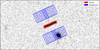 |
Fig. 4 Example streak with apertures placed along the direction of motion of the asteroid to increase the temporal resolution of the sampling. A bright galaxy falls on several of the background apertures; the approach to address it is described in Sect. 4.1. |
 |
Fig. 5 Cut-out of VIS image comprising (left) and the same image with the overlaid mask of cosmic rays in red (right). |
 |
Fig. 6 Light curve of asteroid (18957) Mijacobsen. The time range covers several rotations; however, the sampling intervals are highly regular, which can potentially cause period aliases (a possibility discussed in Sect. 4.2.4). Each data cluster and colour corresponds to a different streak of origin. |
4.2 Period determination
4.2.1 Preliminary vetting
In certain cases, either because the coverage is too short or because the amplitudes of the light curves are smaller than the measurement uncertainties, the light curves do not contain enough signal to constrain a period. As is shown in Fig. 9, we flag these cases by fitting a constant through each light curve; whenever the reduced chi-square, ![Mathematical equation: $\[\chi_{\nu}^{2}\]$](/articles/aa/full_html/2026/06/aa59419-26/aa59419-26-eq6.png) , is 2 or below, we discard the light curve for period analysis. We also discarded light curves with temporal coverage below 1 h after observing that in these rare cases, the algorithm always fits the noise instead of the data. The discarded light curves are presented in Appendix B. We find that using this conservative threshold flags cases that lack enough variability for the period search. We then searched for rotation signatures in the light curves using a three-stage approach: Lomb–Scargle periodogram for initial period estimation, maximum a posteriori (MAP) optimisation to refine the estimate, and Bayesian inference with Markov chain Monte Carlo (MCMC) to find the best value.
, is 2 or below, we discard the light curve for period analysis. We also discarded light curves with temporal coverage below 1 h after observing that in these rare cases, the algorithm always fits the noise instead of the data. The discarded light curves are presented in Appendix B. We find that using this conservative threshold flags cases that lack enough variability for the period search. We then searched for rotation signatures in the light curves using a three-stage approach: Lomb–Scargle periodogram for initial period estimation, maximum a posteriori (MAP) optimisation to refine the estimate, and Bayesian inference with Markov chain Monte Carlo (MCMC) to find the best value.
 |
Fig. 7 Light curve of asteroid 2000 SQ24. The time range covers less than one full rotation, which makes the spin-period determination highly suspect. Each data cluster and colour corresponds to a different streak of origin. |
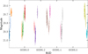 |
Fig. 8 Light curve of asteroid 2005 RE29. The time range covers several rotations, which allows for reliable spin-period determination. Each data cluster and colour corresponds to a different streak of origin. |
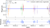 |
Fig. 9 Light curve of asteroid 2010 ES89 fitted by a constant. The data are coloured by streak of origin. The fit is adequate, which implies that the data do not have enough signal to allow for a high-quality period search. We discarded this light curve. |
4.2.2 Lomb–Scargle pre-search
As is discussed in Sect. 1, the Lomb–Scargle algorithm is more robust than simple Fourier analysis for unevenly sampled time series (VanderPlas 2018), which is generally the case for asteroid light curves. It is often applied to infer a period that is used as an initial guess when optimising the model or refined using other search methods, such as MCMC. In the case of the Euclid asteroids, the number of data points, the number of observations, and the data sparsity can vary from one object to another, which makes the use of the Lomb–Scargle method preferable. We used the nifty-ls method developed by Garrison et al. (2024), which is faster and more accurate than the default Astropy implementation. We used the power spectrum from the Lomb–Scargle estimation to set the bounds for the subsequent search, which ranges from 0.5–2.0 times the Lomb–Scargle period.
4.2.3 Bayesian inference via MCMC
Following the approach discussed in Foreman-Mackey et al. (2013), we improved the parameter estimates before the MCMC run by optimising the posterior in two stages. We first explored the parameter space with a global search using differential evolution within the bounds of the prior. Then, the best candidates were locally refined using an L-BFGS-B optimiser (Byrd et al. 1995). The result of this MAP estimate was used to initialise the MCMC walkers. This step does not impose any bounds on the search, but we observe it improves the convergence of the MCMC search.
After that preliminary optimisation had provided sensible starting values for the model parameters, we explored their full posterior distribution using Bayesian inference and the equations laid out in Sect. 3. This approach allowed us to quantify parameter uncertainties and correlations, and to assess the quality of the final model. To build our chains, we used the affineinvariant ensemble sampler implemented in the emcee package developed in Foreman-Mackey et al. (2013). In practice, each MCMC run was initialised near the parameter values found by the MAP optimiser, with small random perturbations to ensure there is diversity among the walkers. We followed the recommendations of the emcee documentation, which suggests using move mixtures to favour transitions between modes in multimodal posteriors. The lower bound for the period was 0.02 days (approximately 30 min) to include possible fast rotators. Faster periods are possible (see Greenstreet et al. 2026), but we expect them only very rarely in our target population, and we observe that reducing the lower bound causes the algorithm to fit the noise. The upper bound was set individually for each asteroid at twice the coverage of the observations; it should be noted that for periods found to be greater than the coverage, the result must be taken with caution and follow-up observations are required. We used 16 walkers, a number that exceeds twice the number of dimensions fitted, which is a requirement laid out in the emcee documentation. The samples of all jointly evaluated parameters represent the posterior distribution. We evolved the walkers for 100 000 steps, which is at least an order of magnitude greater than the estimated integrated autocorrelation time of the chains to ensure stable posterior estimates. We observe that increasing the number of steps beyond that value does not significantly affect the MCMC results, indicating that the chains converge well with the chosen value.
4.2.4 Best period and aliases
Particularly for light curves with large gaps or few data points, the spin-period solution can be degenerate, and the MCMC chain can have multiple modes, known as aliases. This is illustrated in Fig. 11. In such multimodal cases, our data do not fully constrain the model, leaving multiple possible solutions for the period. To account for this, we take the median of the samples assigned to the most likely mode and report those parameters as the best fit. We also report all modes containing more than 5% of the samples as period aliases. The uncertainty of each mode, 1 σ, is taken as the 16th–84th percentile range of the samples assigned to that mode.
4.3 Performance assessment
We first evaluated the quality of our estimates using a phase-dispersion metric. The phase dispersion can quantify whether the data cluster adequately when folded at a given period without assuming a specific model. We folded the light curves by the best period such that we map all points onto the phase interval [0, 1). Grouping the points in bins of ten points, we computed the average of the variances inside each bin, σ2, and compared it to the overall variance of the folded light curve, s2. Considering that we use bins with equal number of points, our definition of the phase dispersion, Θ, is equivalent to that laid out in Stellingwerf (1978),
![Mathematical equation: $\[\Theta=\frac{\sigma^2}{s^2}.\]$](/articles/aa/full_html/2026/06/aa59419-26/aa59419-26-eq7.png) (5)
(5)
A value of Θ close to 0 indicates an extraordinary good fit, whereas Θ close to 1 suggests a poor period estimate. We establish a threshold of Θ = 0.8, above which we observe that the phase-folded light curves do not have a meaningful structure and discard them (although we still publish them in Appendix B). We report the Θ associated with the remaining periods to express, in each case, the reliability of our estimate. In addition, we report the phase coverage, ϕc, which quantifies what fraction of the rotation is sampled by our data. To calculate it, we divide the phase-folded light curve in ten equal bins and compute how many contain data points. In cases where ϕc is below 0.5, the fitted period should be interpreted with caution.
5 Results and discussion
5.1 Pipeline validation
We validated the performance of our pipeline by comparing our period estimates and their aliases with those published in the literature. We relied on real data to validate our method since there are no simulated datasets containing asteroid periods for Euclid. We chose to use the comprehensive Virtual Observatory web service Solar system Open Database Network (SsODNet) because it offers free access to a compilation of more than 3000 articles constantly being updated (see Appendix C), including millions of SSO parameters (Berthier et al. 2023). We accessed the server via the rocks Python client1. Whenever an object has multiple peer-reviewed periods in SsODNet, we selected the closest match. Since the period quality flag is only available for a subset of the periods, we did not discard objects that had a low-quality flag. Only 60 of the periods in our final catalogue have been published by any of the sources in SsODNet, and we do not attempt a comparison with the periods that are more than twice our coverage using Euclid, which reduces the sample to 48 periods, all shown in Table A.1. We include the average magnitude, ⟨m⟩, which is calculated by converting C into magnitude, and the peak-to-peak amplitude, Ap–p, calculated using C and A. In cases in which our A is strongly overestimated and the calculation fails, we report a conservative Ap–p calculated as the difference in magnitude between the maximum and minimum flux. In these and other cases where the amplitude approaches 1 mag, the adopted light curve model does not reliably predict the amplitude, but this does not affect the validity of the period. None of the known periods had Θ above 0.8.
We compared our spin periods with all published periods in the database and the first few integer harmonics of the published periods: 2Past, 3Past, 4Past, and their inverses Past/2, Past/3, and Past/4. Since harmonics convey physically equivalent descriptions of the same rotation state, the period can be reported in SsODNet with one of the harmonics, but represent an identical rotation. As opposed to aliases, which arise from sparse data, period harmonics are indistinguishable from each other; a rotation of period Past with a two-peak shape would present the same light curve as a rotation of period Past/2. Of the 48 matches with the database, a quarter (25.0%) of the periods have the closest match with a harmonic of the published period. For consistency, we report twice the fitted sine period, corresponding to a double-peaked light curve, although we note the harmonics and the fundamental period are mathematically equally valid solutions that cannot be distinguished solely from the photometry.
In cases in which our periods are multimodal, we compare the published period with all aliases. In this development, we confirm that none of the parameters can provide an unequivocal identification of a specific alias as the true value. For instance, the MCMC run performed on asteroid (12776) Reynolds can converge to three different modes, 0.16 days (the published value), 0.08 days (a harmonic of the published value), and 0.06 days. The resultant posterior distribution can be seen as a corner plot in Fig. 10, which shows three distinctive peaks in the period–period panel corresponding to the half period of the asteroid. Figure 11 illustrates why the three aliases cannot be unequivocally distinguished: the large and regular gaps between the different data clusters, corresponding to different observations, allow for the presence of multiple sine peaks. The first mode allows for three peaks in each data gap, the second allows for two, and the third allows for one. The third mode of 0.16 days, the published value, is the most likely fit in this case, but we observe that our best mode is not always the one closest to the published value.
More specifically, we note that in many of the cases, the mode closest to the published value is not necessarily the most likely or the one whose fit produced the best ![Mathematical equation: $\[\chi_{\nu}^{2}\]$](/articles/aa/full_html/2026/06/aa59419-26/aa59419-26-eq8.png) . However, using the full subset of published periods, we find a correlation between the likelihood of the reported modes and the distance to the published value: in 75% of the cases, the closest match is found with the most likely mode, and in 98% of the cases, with one of the three most likely modes; in other words, we establish a 98% confidence that the best solution can be found among the first three most likely modes.
. However, using the full subset of published periods, we find a correlation between the likelihood of the reported modes and the distance to the published value: in 75% of the cases, the closest match is found with the most likely mode, and in 98% of the cases, with one of the three most likely modes; in other words, we establish a 98% confidence that the best solution can be found among the first three most likely modes.
Figure 12 shows the location of the fitted periods with respect to their published value. All modes found for a given period are connected by a line. The size of the points is proportional to their Θ, where a smaller size implies a better fit, while a darker shade of blue correlates with a brighter apparent magnitude. Figure 13 is a version of Fig. 12 with the modes collapsed to the mode closest to the published value or one of its harmonics.
After analysing the parameter distribution of the subsample, we find no clear correlation between the length of the fitted period and its divergency from the published value, as is shown in Fig. 14. We note that 1999 JA and 2001 RB71, the only two cases with discrepancies greater than 20%, also have ϕc values below 0.5, which indicates that they are highly suspect.
We also inspect the relationship with Θ, shown in Fig. 15. Although the range of Θ values in this subset is not wide enough to extract strong conclusions, the plot shows a broad half-trumpet shape, indicating a possible correlation. The outlier to this trend in the top left corner of the figure is one of the objects with low ϕc, 1999 JA. The rest of the parameters, such as the number of data points, the relative amplitude of the data, the absolute and apparent magnitude of the asteroid, and the value of ![Mathematical equation: $\[\chi_{\nu}^{2}\]$](/articles/aa/full_html/2026/06/aa59419-26/aa59419-26-eq9.png) do not show consistent trends and we did not use them to predict the similarity with the published period.
do not show consistent trends and we did not use them to predict the similarity with the published period.
Taking the published periods as the ground truth, we derived statistics on our accuracy. Looking at the central values, 44% of our periods are within 1% of the published period (or one of its harmonics), 65% within 3%, 73% within 5%, and 94% within 15%. To compare our results with similar previous literature, Lam et al. (2023) tested their pipeline by using a dataset of 752 published periods and found that 88% of their periods were within 5% of the published ones. However, our dataset reaches much fainter magnitudes and our approach is sensitive to subthe variations (down to 0.1 mag), while their pipeline requires a magnitude variation of at least 0.3 mag to be detectable. The tests of Waszczak et al. (2015) on 927 periods showed that 67% of their periods were within 3% of the published, a comparable result to ours but for brighter magnitudes, centred around 19 mag. Although our validation sample size is smaller than that reported in the literature, we appear to achieve similar accuracy results for much fainter objects.
In addition, we should note that, even though we set the published periods as the ground truth, in some cases our data from the EES are more densely sampled and have better resolution than the published data using ground-based telescopes. Given that the Euclid telescope is not affected by atmospheric conditions, it is likely that some of our fitted periods are closer to the true value than those published. Whenever available, the quality code U illustrates the level of confidence of the value published in the literature: 3 and 3− do not allow for other solutions; although unlikely, 2+ might be in error; 2 may be wrong by 30%, and 2− indicates that the coverage was not enough to derive an accurate period.
Lastly, we rerun our fitting algorithm by adding a second term to the light curve model in Eq. (2) to assess whether the sinusoidal assumption held. We find that with the additional term, the MCMC routine struggles to converge to reasonable solutions and often overfits the data. This test confirms that in the particular case of our EES data, the simpler single-term model is sufficient.
 |
Fig. 10 Posterior distributions found during an MCMC search for asteroid (12776) Reynolds. The Past/2 panels show three clear modes for the period, which correspond to period aliases. In this case, the data have failed to constrain a unique solution. The range plotted is centred on the posterior and only a fraction of the searched space. |
 |
Fig. 11 Overlay of the three period aliases found in an MCMC run for asteroid (12776) Reynolds. Each data cluster and colour corresponds to a different streak of origin. Mode 3 is the most likely, followed by mode 2 and mode 1. |
 |
Fig. 12 Fitted Past, noted as Pfitted, against the published Past, noted as Ppublished, used for validating the pipeline. In cases presenting period aliases, the different modes are linked by a straight vertical line. The central, continuous red line indicates perfect agreement, while the dashed lines indicate agreement with a harmonic of the published period. The size of the points is proportional to their Θ, where a smaller size implies a better fit. The blue shading of the points indicates their average apparent magnitude, ⟨m⟩. |
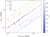 |
Fig. 13 Same as Fig. 12 but with the cases presenting aliases collapsed to the alias closest to the published period or its harmonics. |
 |
Fig. 14 Absolute fractional difference between Ppublished (or, when applicable, the harmonic of the published period that was used for the comparison) and Pfitted as a function of Pfitted. |
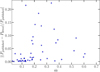 |
Fig. 15 Absolute fractional difference between Ppublished and Pfitted as a function of Θ. |
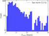 |
Fig. 16 Distribution of all 889 fitted periods in bins of 1 h. The distribution is denser for periods shorter than 1 day and shows an artificial peak in values near 2 days, resulting from the upper bound of the period search. In cases of multimodality, we plot the most likely period. The dashed black line shows the spin barrier at 0.092 days. |
5.2 Period determination for known objects with unknown periods
After validating the performance of our pipeline, we use it to analyse the full dataset of 2321 known objects identified in the EES. Following the criteria described in Sect. 4, we discard 1125 of them because they are unsuited for our period analysis, and 202 after the period finding because they have Θ above 0.8. Given their size, we expect only a minority of our target asteroids to have periods below the spin barrier of 2.2 h, which implies that periods found in this range are more likely to be mistaken. We observe that in short periods for which the value of Θ is high, the algorithm has often fitted the noise. For this reason, we apply an additional filter and discard periods below the spin barrier that have Θ above 0.5 (see Appendix B). This further removes 105 asteroids from the sample, resulting in a dataset of 889 objects: in this subset, five are Mars crossers, four Cybele, four Hilda, three Hungaria, and 877 are located in other regions of the MB. We present a preview of the results in Table A.2; the remaining results are available as an electronic table at the Strasbourg Astronomical Data Center (CDS).
We observe that most of our periods (76%) present aliases, likely due to insufficient phase coverage caused by the cadence of our exposures. Even though the sampling pattern of the EES is dense, it is highly regular, which may lead to repeated gaps that can result in aliasing. We analyse the phase coverage in our sample and find that the average ϕc is 0.64, with a standard deviation of 0.19. Only a small fraction (9%) of the periods have full phase coverage, while 15% of the periods have ϕc below 0.5, which makes them highly suspect. To inform the reader, we include ϕc in Table A.2.
The filtered period distribution in hours is shown in Fig. 16, where we can observe that most periods are concentrated in the range below 1 day. The distribution presents a peak in its tail in longer values, artificially caused by the imposed upper bound on the period search, although the underlying periods could be longer. As such, periods near that value are likely longer in reality. We compared our period distribution with the published database using the Kolmogorov–Smirnov (K–S) test (Massey 1951) and found that the two distributions are compatible, differing by at most 6% in cumulative fraction, as can be seen in Fig. 19. These subtle differences are expected and likely due to selection effects.
We then inspected the distribution of the fitted frequency in our sample as a function of the reported absolute magnitude. We plot the full catalogue of spins in the database in Fig. 17. Similarly to the case of Fig. 16, we observe an overly dense region in the band corresponding to the upper bound. Most of our asteroids have an absolute magnitude 15–19, which corresponds to a diameter size of approximately 1–5 km, assuming typical MB distances and albedo. We performed another K–S test to compare our frequency–magnitude distribution to that of the catalogue, and find that the two distributions differ, even after applying the cuts. As can be seen in Fig. 18, although the distribution of the EES is contained within the bounds of the published distribution, their shapes differ. On average, the objects of the EES are significantly fainter than those published in the catalogue, with cumulative differences of up to 55%. Given that the Euclid mission reaches fainter magnitudes than most dedicated asteroid surveys, this behaviour is expected.
The second quality test we performed was to assess the reliability of the Θ indicator. We visually confirm that whenever Θ is above 0.8, the fit is almost random and we cannot reliably constrain the period of the asteroid. Figure 20 displays several cases of periods with high Θ. The first example shows some structure following the model; however, half of the data points are not aligned with it. The second and fourth examples show signs of variability, but the solutions are clearly not constrained by the data. In the third example, the data are highly dispersed and do not follow the model. We also establish that there is a correlation between low Θ values and higher-quality periods. In contrast to Fig. 20, Fig. 21 shows four examples with low Θ, all visually accurate. Two thirds (64%) of the fitted periods have Θ below 0.5.
Within the filtered periods, we find 16 that are below the spin barrier of 2.2 h. We observe that the light curves in this sample deviate from the first-order sinusoidal shape. This behaviour is expected from the increased rotation speed, which can lead to the presence of binary companions or rotation about an axis other than the principal axis (tumbling). We note that these objects are candidates for being fast rotators since they are below the spin barrier and, given their large size (all below absolute magnitude 19), they are considered candidate super-fast rotators. The rate found of approximately 0.5% (16/2321) is consistent with the literature (Strauss et al. 2024). The full list of candidates can be found in Table A.3, and four example phase-folded light curves are depicted in Fig. 22. The case of 1992 RC4, 1999 XN26 and 2000 GP60 is particularly rare for their large size: 3.0 km (absolute magnitude 14.8). Since the Euclid sampling for these asteroids is sparse for such short periods, we will require followup observations to further constrain their rotation periods and confirm their status as super-fast rotators.
We built an open database containing the light curves of all 2321 objects studied, all period results, including the 889 high-quality periods, and their most relevant physical parameters. This information will allow all users of our catalogue to interpret and use our data appropriately.
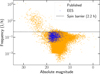 |
Fig. 17 Distribution of all 889 fitted periods in the context of the known distribution, from the literature. The dashed black line shows the spin barrier at 0.092 days. |
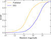 |
Fig. 18 One-dimensional K–S test comparing the empirical cumulative distribution functions (ECDFs) of our magnitude distribution and the published over the same period-magnitude range. The two distributions diverge, with cumulative differences of up to 55%. As expected, the EES objects are fainter. |
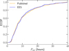 |
Fig. 19 One-dimensional K–S test comparing the empirical cumulative distribution functions (ECDFs) of our period distribution and the published one. The two distributions are found to be broadly consistent, with a maximum difference between the two cumulative distributions of 6%. |
 |
Fig. 20 Examples of phase-folded light curves using periods with Θ above 0.8, indicating a poor solution. All cases with Θ above 0.8 are discarded from the results. From top to bottom: 1996 RC17, 2000 KW84, 2001 MR3, and 2002 GP193. |
6 Conclusions and future work
We present a catalogue of spin periods for 889 MB asteroids observed during the EES, which took place at the beginning of the Euclid mission. This is the first set of spin periods extracted from Euclid light curves. The photometric precision and long exposures of the VIS images have allowed us to build dense light curves for many objects for which only sparse photometry was available before. Out of the 889 spin periods, 93% (829) had never been reported before. We validate the performance of our pipeline by comparing our fitted periods with the values published in the SsODNet database for the 48 cases with sufficient Euclid coverage. We find that in 44% of the cases, our fitted period is within 1% of the value published in the literature or one of its harmonics, and that 98% of our periods are within 15% of the published value. For the cases analysed, the largest driver of divergence from the published period is the phase coverage, and other parameters, such as goodness of fit, magnitude, or amplitude, have only a marginal effect.
With this work, we have aimed to expand our knowledge of the spin-period distribution in the MB and to complement, and even improve, the efforts of ground-based telescopes. Future work will focus on extracting the rotation periods of unknown objects observed during the EES by first linking their streaks across multiple observations. To strengthen our findings, we will incorporate data taken with other surveys. We will also work on upcoming detections from the Euclid Wide Survey, which will provide sparser data but a higher likelihood of encountering near-Earth asteroids. This new dataset will enable us to test our pipeline on a different asteroid population and potentially shorter rotation periods. As the Euclid Wide Survey unfolds during the nominal six-year mission, we will expand our catalogue of asteroid rotational properties in future data releases.
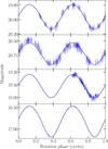 |
Fig. 21 Examples of phase-folded light curves using periods with Θ below 0.1, indicating an excellent solution. From top to bottom: 2000 VW31, 2006 WG108, (18957) Mijacobsen, and (2165) Young. |
 |
Fig. 22 Candidate super-fast rotators, with periods below 2.2 h. From top to bottom: 2005 SS44, 2013 SG64, 2015 XS290, and 2023 TC192. |
Data availability
The data used for this study will become available in November 2026 with the DR1 (Euclid Data Release 1 2026). The full Tables A.2, B.1, and B.2 are available at the CDS via https://cdsarc.cds.unistra.fr/viz-bin/cat/J/A+A/710/A27.
Acknowledgements
We thank Marco Micheli, Odysseas Xenos, and the anonymous reviewer for their helpful comments. This project has received funding from the European Union’s Horizon 2020 and Horizon Europe research and innovation programmes under the Marie Skłodowska-Curie grant agreement Nos. 945363 and 101105725, and funding from the Swiss National Science Foundation and the Swiss Innovation Agency (Innosuisse) via the BRIDGE Discovery grant 40B2-0 194729. This research makes use of ESA Datalabs (datalabs.esa.int), an initiative by ESA’s Data Science and Archives Division in the Science and Operations Department, Directorate of Science. The Euclid Consortium acknowledges the European Space Agency and a number of agencies and institutes that have supported the development of Euclid, in particular the Agenzia Spaziale Italiana, the Austrian Forschungsförderungsgesellschaft funded through BMK, the Belgian Science Policy, the Canadian Euclid Consortium, the Deutsches Zentrum für Luft- und Raumfahrt, the DTU Space and the Niels Bohr Institute in Denmark, the French Centre National d’Etudes Spatiales, the Fundação para a Ciência e a Tecnologia, the Hungarian Academy of Sciences, the Ministerio de Ciencia, Innovación y Universidades, the National Aeronautics and Space Administration, the National Astronomical Observatory of Japan, the Netherlandse Onderzoekschool Voor Astronomie, the Norwegian Space Agency, the Research Council of Finland, the Romanian Space Agency, the State Secretariat for Education, Research, and Innovation (SERI) at the Swiss Space Office (SSO), and the United Kingdom Space Agency. A complete and detailed list is available on the Euclid web site (https://www.euclid-ec.org).
References
- Barnouin, O. S., Daly, M. G., Palmer, E. E., et al. 2019, Nat. Geosci., 12, 247 [Google Scholar]
- Bellm, E. C., Kulkarni, S. R., Graham, M. J., et al. 2018, PASP, 131, 018002 [Google Scholar]
- Berthier, J., Carry, B., Mahlke, M., & Normand, J. 2023, A&A, 671, A151 [NASA ADS] [CrossRef] [EDP Sciences] [Google Scholar]
- Berthier, J., Vachier, F., Thuillot, W., et al. 2006, in Astron. Data Anal. Softw. Syst. XV, 351, 367 [Google Scholar]
- Byrd, R. H., Lu, P., Nocedal, J., & Zhu, C. 1995, SIAM J. Sci. Comput., 16, 1190 [Google Scholar]
- Carry, B. 2018, A&A, 609, A113 [NASA ADS] [CrossRef] [EDP Sciences] [Google Scholar]
- Cellino, A., Tanga, P., Muinonen, K., & Mignard, F. 2024, A&A, 687, A277 [NASA ADS] [CrossRef] [EDP Sciences] [Google Scholar]
- Chang, C.-K., Ip, W.-H., Lin, H.-W., et al. 2015, ApJS, 219, 27 [NASA ADS] [CrossRef] [Google Scholar]
- Chang, C.-K., Lin, H.-W., Ip, W.-H., et al. 2016, ApJS, 227, 20 [Google Scholar]
- Chang, C.-K., Lin, H.-W., Ip, W.-H., et al. 2017, Geosci. Lett., 4, 17 [Google Scholar]
- Chang, C.-K., Lin, H.-W., Ip, W.-H., et al. 2019, ApJS, 241, 6 [Google Scholar]
- Clement, M. S., Morbidelli, A., Raymond, S. N., & Kaib, N. A. 2020, MNRAS, 492, L56 [NASA ADS] [CrossRef] [Google Scholar]
- Conversi, L., Licandro, J., Delbo, M., et al. 2024, in Space Telescopes and Instrumentation 2024: Optical, Infrared, and Millimeter Wave, 13092, SPIE, 943 [Google Scholar]
- Devogèle, M., Buzzi, L., Micheli, M., et al. 2024, A&A, 689, A211 [NASA ADS] [CrossRef] [EDP Sciences] [Google Scholar]
- Ďurech, J., & Hanuš, J. 2023, A&A, 675, A24 [NASA ADS] [CrossRef] [EDP Sciences] [Google Scholar]
- Ďurech, J., Hanuš, J., & Ali-Lagoa, V. 2018, A&A, 617, A57 [NASA ADS] [CrossRef] [EDP Sciences] [Google Scholar]
- Ďurech, J., Vávra, M., Vančo, R., & Erasmus, N. 2022, Front. Astron. Space Sci., 9, 809771 [Google Scholar]
- Eglitis, I., & Svincicka, D. 2025, Icarus, 428, 116380 [Google Scholar]
- Erasmus, N., Navarro-Meza, S., McNeill, A., et al. 2020, ApJS, 247, 13 [CrossRef] [Google Scholar]
- Erasmus, N., Kramer, D., McNeill, A., et al. 2021, MNRAS, 506, 3872 [NASA ADS] [CrossRef] [Google Scholar]
- Euclid Collaboration (Scaramella, R., et al.) 2022, A&A, 662, A112 [NASA ADS] [CrossRef] [EDP Sciences] [Google Scholar]
- Euclid Collaboration (Cropper, M., et al.) 2025, A&A, 697, A2 [Google Scholar]
- Euclid Collaboration (Jahnke, K., et al.) 2025, A&A, 697, A3 [Google Scholar]
- Euclid Collaboration (McCracken, H. J., et al.) 2026, A&A, in press, https://doi.org/10.1051/0004-6361/202554594 [Google Scholar]
- Euclid Collaboration (Mellier, Y., et al.) 2025, A&A, 697, A1 [Google Scholar]
- Euclid Data Release 1. 2026, https://doi.org/10.57780/esa-d079c51 [Google Scholar]
- Foreman-Mackey, D., Hogg, D. W., Lang, D., & Goodman, J. 2013, PASP, 125, 306 [Google Scholar]
- Fraser, W., Alexandersen, M., Schwamb, M. E., et al. 2016, AJ, 151, 158 [NASA ADS] [CrossRef] [Google Scholar]
- Garrison, L. H., Foreman-Mackey, D., Shih, Y.-H., & Barnett, A. 2024, Res. Notes AAS, 8, 250 [Google Scholar]
- Gómez-Alvarez, P., Dupac, X., Buenadicha, G., et al. 2018, in Software and Cyberinfrastructure for Astronomy V, 10707, SPIE, 285 [Google Scholar]
- Granvik, M., Morbidelli, A., Vokrouhlickỳ, D., et al. 2017, A&A, 598, A52 [NASA ADS] [CrossRef] [EDP Sciences] [Google Scholar]
- Greenstreet, S., Li, Z., Vavilov, D. E., et al. 2026, ApJ, 996, L33 [Google Scholar]
- Harris, A. W., Young, J. W., Bowell, E., et al. 1989, Icarus, 77, 171 [NASA ADS] [CrossRef] [Google Scholar]
- Hirabayashi, M., Sánchez, D. P., & Scheeres, D. J. 2015, ApJ, 808, 63 [NASA ADS] [CrossRef] [Google Scholar]
- Kaiser, N., Aussel, H., Burke, B. E., et al. 2002, in Survey and Other Telescope Technologies and Discoveries, 4836, SPIE, 154 [Google Scholar]
- Kelly, B. C. 2007, ApJ, 665, 1489 [Google Scholar]
- Lagerros, J. S. V. 1996, A&A, 310, 1011 [Google Scholar]
- Lam, A. L. H., Margot, J.-L., Whittaker, E., & Myhrvold, N. 2023, Planet. Sci. J., 4, 61 [Google Scholar]
- Magnusson, P. 1991, A&A, 243, 512 [NASA ADS] [Google Scholar]
- Mainzer, A. K., Masiero, J. R., Abell, P. A., et al. 2023, Planet. Sci. J., 4, 224 [Google Scholar]
- Marciniak, A., Ali-Lagoa, V., Müller, T. G., et al. 2019, A&A, 625, A139 [NASA ADS] [CrossRef] [EDP Sciences] [Google Scholar]
- Marzari, F., Rossi, A., Golubov, O., & Scheeres, D. J. 2020, AJ, 160, 128 [NASA ADS] [CrossRef] [Google Scholar]
- Massey, F. J. J., 1951, J. Am. Stat. Assoc., 46, 68 [CrossRef] [Google Scholar]
- McCully, C., Crawford, S., Kovacs, G., et al. 2018, https://doi.org/10.5281/zenodo.1482019 [Google Scholar]
- McNeill, A., Gowanlock, M., Mommert, M., et al. 2023, AJ, 166, 152 [NASA ADS] [CrossRef] [Google Scholar]
- Müller, T. G., & Lagerros, J. S. V. 1998, A&A, 338, 340 [NASA ADS] [Google Scholar]
- Nucita, A. A., Conversi, L., Verdier, A., et al. 2025, A&A, 694, A116 [NASA ADS] [CrossRef] [EDP Sciences] [Google Scholar]
- Ostro, S. J., Hudson, R. S., Jurgens, R. F., et al. 1995, Science, 270, 80 [Google Scholar]
- Pál, A., Szakáts, R., Kiss, C., et al. 2020, ApJS, 247, 26 [CrossRef] [Google Scholar]
- Persson, B. N. J., & Biele, J. 2022, Tribol. Lett., 70, 34 [Google Scholar]
- Podlewska-Gaca, E., Poleski, R., Bartczak, P., McDonald, I., & Pál, A. 2021, ApJS, 255, 4 [Google Scholar]
- Polishook, D., Ofek, E. O., Waszczak, A., et al. 2012, MNRAS, 421, 2094 [Google Scholar]
- Pöntinen, M., Granvik, M., Nucita, A. A., et al. 2020, A&A, 644, A35 [NASA ADS] [CrossRef] [EDP Sciences] [Google Scholar]
- Pöntinen, M., Granvik, M., Nucita, A., et al. 2025, Asteroid Science with ESA Euclid: Results from the Ecliptic PDC Campaign, Tech. rep., Copernicus Meetings [Google Scholar]
- Pravec, P., Harris, A. W., & Michalowski, T. 2002, Asteroids III, 113, 35 [Google Scholar]
- Pravec, P., Scheirich, P., Kušnirák, P., et al. 2006, Icarus, 181, 63 [NASA ADS] [CrossRef] [Google Scholar]
- Rozitis, B., & Green, S. F. 2011, MNRAS, 415, 2042 [NASA ADS] [CrossRef] [Google Scholar]
- Rubincam, D. P. 2000, Icarus, 148, 2 [Google Scholar]
- Scheeres, D. J., Fahnestock, E. G., Ostro, S. J., et al. 2006, Science, 314, 1280 [NASA ADS] [CrossRef] [Google Scholar]
- Sergeyev, A. V., Carry, B., Eggl, S., et al. 2025, A&A, 703, A302 [NASA ADS] [CrossRef] [EDP Sciences] [Google Scholar]
- Spencer, J. R., Lebofsky, L. A., & Sykes, M. V. 1989, Icarus, 78, 337 [Google Scholar]
- Stellingwerf, R. F. 1978, ApJ, 224, 953 [Google Scholar]
- Stephens, R. D. 2012, Minor Planet Bull., 39, 80 [Google Scholar]
- Strauss, R., McNeill, A., Trilling, D. E., et al. 2024, AJ, 168, 184 [Google Scholar]
- Szabó, G. M., Pál, A., Szigeti, L., et al. 2022, A&A, 661, A48 [NASA ADS] [CrossRef] [EDP Sciences] [Google Scholar]
- Taylor, P. A., Margot, J.-L., Vokrouhlicky, D., et al. 2007, Science, 316, 274 [NASA ADS] [CrossRef] [Google Scholar]
- Tonry, J. L., Denneau, L., Heinze, A. N., et al. 2018, PASP, 130, 064505 [Google Scholar]
- VanderPlas, J. T. 2018, ApJS, 236, 16 [Google Scholar]
- Vavilov, D. E., & Carry, B. 2025, A&A, 693, A66 [NASA ADS] [CrossRef] [EDP Sciences] [Google Scholar]
- Virtanen, J., Poikonen, J., Säntti, T., et al. 2016, Adv. Space Res., 57, 1607 [NASA ADS] [CrossRef] [Google Scholar]
- Waszczak, A., Chang, C.-K., Ofek, E. O., et al. 2015, AJ, 150, 75 [NASA ADS] [CrossRef] [Google Scholar]
- Wiktorowicz, S., & Masiero, J. R. 2017, in AAS/Division for Planetary Sciences Meeting Abstracts, 49, 110.32 [Google Scholar]
- Wright, E. L., Eisenhardt, P. R. M., Mainzer, A. K., et al. 2010, AJ, 140, 1868 [Google Scholar]
- Yeh, T.-S., Li, B., Chang, C.-K., et al. 2020, AJ, 160, 73 [NASA ADS] [CrossRef] [Google Scholar]
Appendix A Tables
We present in Table A.1 a comparison between our fitted periods and those reported in the SSODNet catalogue; in Table A.2, a preview of the fitted periods from the EES, and in Table A.3, the candidate super-fast rotators in the EES. For a detailed discussion, see Sect. 5.1 and Sect. 5.2.
Comparison between our fitted periods and those reported in the SSODNet catalogue.
Fitted periods from the EES (preview).
Candidate super-fast rotators in the EES.
Appendix B Discarded light curves
We present in Table B.1 a preview of the light curves that did not show enough variability in the observed time range to allow for period determination. A description of the methods used for this filtering can be found in Sect. 4.2. We present in Table B.2 period fits that we considered low quality and excluded from the sample of 889 high-quality periods, as is discussed in Sect. 4.3.
Light curves from the EES that did not show variability (preview).
Periods from the EES that were considered low-quality fits (preview).
Appendix C Sources of known periods used
We present the sources of the periods used for comparison with our results in Sect. 5.
Stephens (2012); Chang et al. (2015); Waszczak et al. (2015); Chang et al. (2016); Ďurech et al. (2018); Chang et al. (2019); Erasmus et al. (2020); Pál et al. (2020); Yeh et al. (2020); Podlewska-Gaca et al. (2021); Ďurech et al. (2022); Ďurech & Hanuš (2023); Lam et al. (2023); McNeill et al. (2023); Cellino et al. (2024).
All Tables
Comparison between our fitted periods and those reported in the SSODNet catalogue.
All Figures
|
Fig. 1 Position in ecliptic co-ordinates of the EES (encircled in white) in the context of the DR1 (coloured tiles), projected using the Euclid Survey System (Gómez-Alvarez et al. 2018). The survey took place from 23 to 31 December 2023 and lay on the ecliptic plane, since it was designed to approximately follow the motion of the asteroids in the MB. A detail of the survey can be seen in Fig. 2. |
| In the text | |
|
Fig. 2 Detail of the observing strategy of the EES, which starts on the rightmost squares on 23 December 2023 (black) and ends on the leftmost squares on 31 December 2023 (pink). Each square corresponds to a single exposure of 560.5 s (dither) and each observation is comprised by four dithers. Within each observation, the four dithers follow an S-shaped pattern. The observations had a high overlap to ensure that the asteroids observed would be seen in as many exposures as possible. In the figure, ecliptic longitude increases from right to left and the ecliptic latitude increases from bottom to top (ecliptic north is up). The Moon is displayed for a scale reference. |
| In the text | |
|
Fig. 3 Diagram summarising the general workflow of our pipeline. We first build our light curves, excluding the outliers and cases with insufficient signal. Then, we search the period using multiple algorithms and, after filtering, compare our results with those published in the catalogue. |
| In the text | |
|
Fig. 4 Example streak with apertures placed along the direction of motion of the asteroid to increase the temporal resolution of the sampling. A bright galaxy falls on several of the background apertures; the approach to address it is described in Sect. 4.1. |
| In the text | |
|
Fig. 5 Cut-out of VIS image comprising (left) and the same image with the overlaid mask of cosmic rays in red (right). |
| In the text | |
|
Fig. 6 Light curve of asteroid (18957) Mijacobsen. The time range covers several rotations; however, the sampling intervals are highly regular, which can potentially cause period aliases (a possibility discussed in Sect. 4.2.4). Each data cluster and colour corresponds to a different streak of origin. |
| In the text | |
|
Fig. 7 Light curve of asteroid 2000 SQ24. The time range covers less than one full rotation, which makes the spin-period determination highly suspect. Each data cluster and colour corresponds to a different streak of origin. |
| In the text | |
|
Fig. 8 Light curve of asteroid 2005 RE29. The time range covers several rotations, which allows for reliable spin-period determination. Each data cluster and colour corresponds to a different streak of origin. |
| In the text | |
|
Fig. 9 Light curve of asteroid 2010 ES89 fitted by a constant. The data are coloured by streak of origin. The fit is adequate, which implies that the data do not have enough signal to allow for a high-quality period search. We discarded this light curve. |
| In the text | |
|
Fig. 10 Posterior distributions found during an MCMC search for asteroid (12776) Reynolds. The Past/2 panels show three clear modes for the period, which correspond to period aliases. In this case, the data have failed to constrain a unique solution. The range plotted is centred on the posterior and only a fraction of the searched space. |
| In the text | |
|
Fig. 11 Overlay of the three period aliases found in an MCMC run for asteroid (12776) Reynolds. Each data cluster and colour corresponds to a different streak of origin. Mode 3 is the most likely, followed by mode 2 and mode 1. |
| In the text | |
|
Fig. 12 Fitted Past, noted as Pfitted, against the published Past, noted as Ppublished, used for validating the pipeline. In cases presenting period aliases, the different modes are linked by a straight vertical line. The central, continuous red line indicates perfect agreement, while the dashed lines indicate agreement with a harmonic of the published period. The size of the points is proportional to their Θ, where a smaller size implies a better fit. The blue shading of the points indicates their average apparent magnitude, ⟨m⟩. |
| In the text | |
|
Fig. 13 Same as Fig. 12 but with the cases presenting aliases collapsed to the alias closest to the published period or its harmonics. |
| In the text | |
|
Fig. 14 Absolute fractional difference between Ppublished (or, when applicable, the harmonic of the published period that was used for the comparison) and Pfitted as a function of Pfitted. |
| In the text | |
|
Fig. 15 Absolute fractional difference between Ppublished and Pfitted as a function of Θ. |
| In the text | |
|
Fig. 16 Distribution of all 889 fitted periods in bins of 1 h. The distribution is denser for periods shorter than 1 day and shows an artificial peak in values near 2 days, resulting from the upper bound of the period search. In cases of multimodality, we plot the most likely period. The dashed black line shows the spin barrier at 0.092 days. |
| In the text | |
|
Fig. 17 Distribution of all 889 fitted periods in the context of the known distribution, from the literature. The dashed black line shows the spin barrier at 0.092 days. |
| In the text | |
|
Fig. 18 One-dimensional K–S test comparing the empirical cumulative distribution functions (ECDFs) of our magnitude distribution and the published over the same period-magnitude range. The two distributions diverge, with cumulative differences of up to 55%. As expected, the EES objects are fainter. |
| In the text | |
|
Fig. 19 One-dimensional K–S test comparing the empirical cumulative distribution functions (ECDFs) of our period distribution and the published one. The two distributions are found to be broadly consistent, with a maximum difference between the two cumulative distributions of 6%. |
| In the text | |
|
Fig. 20 Examples of phase-folded light curves using periods with Θ above 0.8, indicating a poor solution. All cases with Θ above 0.8 are discarded from the results. From top to bottom: 1996 RC17, 2000 KW84, 2001 MR3, and 2002 GP193. |
| In the text | |
|
Fig. 21 Examples of phase-folded light curves using periods with Θ below 0.1, indicating an excellent solution. From top to bottom: 2000 VW31, 2006 WG108, (18957) Mijacobsen, and (2165) Young. |
| In the text | |
|
Fig. 22 Candidate super-fast rotators, with periods below 2.2 h. From top to bottom: 2005 SS44, 2013 SG64, 2015 XS290, and 2023 TC192. |
| In the text | |
Current usage metrics show cumulative count of Article Views (full-text article views including HTML views, PDF and ePub downloads, according to the available data) and Abstracts Views on Vision4Press platform.
Data correspond to usage on the plateform after 2015. The current usage metrics is available 48-96 hours after online publication and is updated daily on week days.
Initial download of the metrics may take a while.